A Risk Management Framework for Industry 4.0 Environment

Abstract

In past decades, manufacturing companies have paid considerable attention to using their available resources in the most efficient way to satisfy customer demands. This endeavor is supported by many Industry 4.0 methods. One of these is called MES (Manufacturing Execution System), which is applied for monitoring and controlling manufacturing by recording and processing production-related data. This article presents a possible method of implementation of a risk-adjusted production schedule in a data-rich environment. The framework is based on production datasets of multiple workshops, which is followed by statistical analysis, and its results are used in stochastic network models. The outcome of the simulation is implemented in a production scheduling model to determine how to assign the production among workshops. After collecting the necessary data, the reliability indicator-based stochastic critical path method was applied in the case study. Two cases were presented based on the importance of inventory cost and two different scheduling results were created and presented. With the objective of the least inventory cost, the production was postponed to the latest time possible, which means that workshops had more time to finish their previous work on the first day due to the small production quantity. When the cost was not relevant, the production started on the first day of each workshop, and the production was completed before the deadline. These are optimal solutions, but alternative solutions can also be performed by the decision maker based on the results. The use of the modified stochastic critical path method and its analysis shed light on the deficiency of the production, which is a merit in the continuous improvement process and the estimation of the total project time.

1. Introduction

Sustainability in production is a great intention of companies—one of its peak points in modern history is the advance of the Toyota Production System (TPS) in Japan [1]. The lack of resources has urged manufacturing companies to produce high-quality products by creating the fewest defective products [1,2]. This attitude aligns with a better understanding of customer needs and conscious usage of raw materials, human and machine power, in short, resources. Due to this production strategy, numerous papers have presented a significant decrease in production cycle time [3] or an increase in machine availability [4], optimizing cost and/or sales indicators [5,6,7], or layout optimization [8] in order with inventory and supermarket decrease and shorter lead times with no extra waste time [9]. A “side effect” of this thorough production is the lower cost implications and lower price for the customer. As reported in [10,11], technology enhancement is a catalyst to the spread of the TPS worldwide because of the data resource. With this available data, much hidden information can be revealed, and well-established decision-making can be made. Parallel with the advent of the Industry 4.0 methodology, customer requirements toward a product or service have increased, and production transparency and traceability have become “must-have” features of a product [12]. Such features require digital transformation and great investment from the company’s side, but this system promotes process improvement opportunities and aids thoughtful production scheduling, which is—in other words—good management of resources. The main objective of this article is to present an approach with the use of which reliability issues can be implemented in the planning phase which bases a fundamental point in the negotiation with the customer and the signature of the final contract. This can result in an increase in the reputation of the company, while the company can avoid paying penalties. The case study presents a practical presentation of a workshop layout and small-batch project scheduling task, where all the workshops work independently but in a project structure. The result of the modified stochastic method supports the scheduling at the factory when the inventory cost plays and does not play a crucial role in the decision making.

2. Literature Background

The main goal of the research is to find a way to implement reliability-based indicators in the stochastic critical path method and its result to be integrated into the process of production scheduling. Since much relevant data is available at many of the companies, Industry 4.0 and a very valuable field, MES, are discussed. In the next subchapters, the fundamentals of risk management in project scheduling are discussed, and the widely used methods are discussed. As an establishment for the result part, the Critical Path Method (CPM) and Stochastic Critical Path Method (SCPM) are briefly presented.

2.1. Industry 4.0 (I4.0) and Manufacturing Execution System (MES)

Industry 4.0 is the terminus of digitalized manufacturing. The automated manufacturing machines are connected to each other and to databases, and all necessary information about the production is recorded and analyzed with the use of I4.0 tools [13,14]. The methodology supports not only environmental sustainability by novel and innovative production techniques (such as additive manufacturing or digital layout planning [8]) but economic (e.g., production cost and efficiency) and social/human perspectives (e.g., ergonomic workplace) are developed as well. With high-tech equipment such as sensors, as well as sophisticated software applications and analysis tools, every aspect of production becomes measurable, from emissions during production to product delivery [12]. Additionally, life cycle assessment becomes more accurate and action plans for changing KPIs (e.g., reducing emissions or increasing profits) become much more predictable when supported by data [15,16].

One of the important modules of Industry 4.0 is Manufacturing Execution System (MES). This is a fundamental component of Industry 4.0 methodology. It supports supervision over production with traceability and real-time production monitoring, as well as controlling production to achieve the desired product in quantity and quality [12,14]. This is carried out by connecting the shopfloor layer (machines, the production and material flow as well as human resources) with the enterprise resource system (where orders and production flows can be found) and by providing helpful, real-time data for decision-makers [13,17]. As an outcome, it facilitates personalized production, which is a value-added factor for customers in fields such as the automotive or electrical industries. Data collection is performed using Internet of Things (IoT) equipment, storing historical data in databases, as well as requiring software from which all the necessary production management-related information (order, production logic, bill of material) can be obtained [12]. The collected information can be analyzed to create capacity plans but is vital for understanding production more in detail and preparing for uncertainties both in the manufacturing process and in the demand [18,19].

MES is not a standalone element of the IT infrastructure; several complementary modules can be attached to the system itself. Furthermore, as can be read in [14], it is advised to build an MES application modular, that is continuously revised and developed to achieve higher performance or efficiency.

Besides the requirements listed by the article [13], new demands arise during the design or implementation of an MES application. One notable feature is discussed by the authors in [14], which is the inclusion of risk management in the prediction. In the same article [14], additional needs were mentioned which are also important to create an environment-conscious system, namely MES, which must provide a system for energy resource control, as well as supervision of dispatch control: assign energy consumption figures to machines or created products.

2.2. Risk Management and Decision-Making under Industry 4.0 Domain

To serve the customers’ needs and support the company’s interests, risk management of certain main processes is needed, and for this request, practical and theoretical tools are also available [20,21]. These tools facilitate a deeper understanding of possible problems during a certain process, support management to think ahead of the problem to reduce the reaction time, and provide flexibility in the decision-making process. Several operations strategies, especially project management, deal with risk management more actively since the project creates a unique output that is too costly to repeat or even rework. Most of the traditional risk management tools are qualitative; however, in a data-rich environment, quantitative methods, such as mathematical risk calculations or simulations, are applied. It is hard to decide which is better, but based on [22], the two approaches can be complementary to each other. Risk matrices as a standalone or complemented with other tools [23] and FMEA [24] are widely accepted and recommended methods—as semi-quantitative tools—in many fields of industry; nevertheless, many research studies have aimed at improving them [24,25,26]. Most of these improvements have been made to make these methods more objective. The main disadvantage of using these tools is that the results cannot be directly implemented in production scheduling because these methods focus on ranking potential risks, not on the time effect on the production.

This can be aligned with the objectives of Industry 4.0 methodology, whose aim is to have full control over the data collection, processing and analysis that relate to the manufacturing process [13]. This goal supports data-driven risk management and data-driven decision-making by providing real-time data for professionals [27]. Not only do professionals benefit from the increased volume of data, but sophisticated tools such as regression modeling (or machine-learning tools) will also be available, and patterns can be identified [28]. Furthermore, one of the most crucial fields, production scheduling, can use the outcome of the accumulated information [29,30]. As many studies show, there is a high need to know when is the most realistic time to produce the right amount of product for the customer, or how production should be allocated to be the quickest [30,31], or the most eco-sustainable [31,32].

2.3. Stochastic Methods for Project Risk Management

As a main project scheduling method, the Critical Path Method (CPM) is used for planning production and investigating potential critical activities, as well as determining the total production time. This network optimization method seeks to find the shortest path of the network ($\min z=x_n-x_1$), while all the activities are carried out totally. The optimization’s sensitivity and other activities enable the decision maker to gather additional and crucial information about the project itself, such as time floats [33,34]. However, as [33,35] report, there are some drawbacks of the method, such as the deterministic approach it uses. This implies that only one scenario can be checked at a time. Another, complementary method is called the Project Evaluation and Review Technique (PERT), but its result can be unreliable because it is based on the result of the CPM technique.

One of the significant inputs of deterministic network planning, i.e., the classic critical path method, is the effect of individual activity times on each other (dependency or prerequisite), as well as the deterministic time data for each activity. One of the assumptions of the stochastic critical path method, based on Schwickert [36], is that the time for each activity $x_1,x_2, \dots x_n$ represents a value $T\left(x_i\right)$ generated from a non-negative random number. Additionally, the maximum time elapsed between two arbitrary nodes of a given stochastic network (i.e., the shortest path during which all activities are performed):

$$D\left(u,v\right)=\underset{\pi \in \prod \left(u,v\right)}{\max }\left\{{\displaystyle \sum }_{\pi }T\left(x_i\right) \right\}$$

(1)

This can be described by the above equation; the purpose of the function is to minimize the total lead time. As described in the article by Yuya et al. [37], the individual activity times are independent of each other, so the change in the time of one activity is not closely correlated with the change in the time of another activity. Badiru’s article [38] presents an alternative to PERT analysis, the stochastic CPM method, and its comparison. The models described in the article work on the basis of historical data.

3. Materials and Methods

3.1. Research Problems, Objectives and Research Questions

Since most of the Industry 4.0-ready machines are equipped with sensors and applications that can communicate via different ports and communication channels, data collection about the production environment has become evident and highly required by the customers to ensure product quality and traceability [13]. Most of the companies are satisfied if the basic modules of MES are working (which is mostly needed directly by the customer), there is no resource or proper method, or just enthusiasm for analyzing data to create a short-term forecast for the production’s capability.

A key to creating such a forecast for production is the proper definition of availability, performance and quality indicators, which are referred to as the Overall Equipment Efficiency (OEE) [19,39]. This indicator originated from the Total Productive Maintenance methodology, which calculates how efficient a machine was in the past. However, it was developed to measure efficiency historically, papers have argued for using it in the future, for the planning phase as well [40].

The Overall Equipment Efficiency is developed for mass manufacturing circumstances, where idle time should not be significant, and improvements can be attempted and conceived [39]. This study focuses on a production environment, where a mix of project and serial production is established: a customer orders a special product in a moderate quantity while the production runs in a workshop format and some teams produce the same amount of product until the required quantity is reached. Such a setup requires well-thought-out production planning and scheduling, which takes the probable risks and uncertainties into account.

The objective of this study is twofold: authors present what data are needed and processed to make decisions, additionally they create a conceptual framework, where the decision-making process is presented. To be coherent, the following questions (RQs) and goals and theses (GTs) are generated:

(GT1) The application of two machine reliability-based indicators in the stochastic critical path method: Mean Time Between Failures (MTBF) and mean downtime.

(GT2) The integration of the modified critical path method’s results into a linear programming method, which provides alternatives to decision-makers in terms of production scheduling. This method would take reliability indicators into account during the planning phase.

To support the hypothesis testing, one research question was defined:

(RQ1) How can MES-based data be implemented in the decision-making process?

(RQ2) Is the combination of risk assessment and product scheduling methodologies providing a proper foundation for decision-makers to define a production schedule?

3.2. Conceptual Framework

3.2.1. Data Collection

A machine or a workstation that supplies information about the production needs an efficient IT infrastructure: software that can communicate with the machine via ports, and a database that stores these data in a structured format with a dashboard that displays real-time as well as historical data. This information is crucial to collect based on the literature [12].

• Cycle time determination:

  ∘

  A trigger is when the product arrived at an exact station or that specific process step. To have accurate data, a unique identification system is needed for the products.

  ∘

  Another trigger is when the product is being processed fully and it is ready to move to or start another activity.

  ∘

  These triggers must be differentiated, so “process_start” and “process_finish” states have to be created. A cycle time is counted between two identical points of production (e.g., between two “process_start” states), but it is also a point to make difference between the process cycle time itself and waiting times, as waiting time is a waste, like it is stated in some lean literature [1].

  ∘

  In the case of physical work, where there is no industry 4.0-ready machine in production, hand scanners with a PC can be utilized. The primary aim is to see how long a certain activity takes with “detailed” reporting. Most of the burden has to be taken off the workers’ shoulders, a system must be implemented which supports reporting and does not cause any extra work for the employees.

• Parameters of production:

  ∘

  When a product is being processed, much information can be collected: environmental parameters, such as temperature or humidity but also machine-related information (specific characteristics from the machine—force, torque, etc.) can be registered. The latter information is vital for determining the quality of the process step, but the prediction of the machine condition or maintenance is feasible in case of proper data collection.

• Breakdown information:

  ∘

  When production is temporarily suspended, information should be given about the characteristic of the downtime to make deeper analyses about the root causes as well as make a prediction for the future.

In the case of workshop layout, multiple workshops work on similar products parallel, the gathered information about a workshop must be distinguished from the other ones; however, it is advised that values must be aggregated for analyses. Because it is hard to find 2 or more totally identical workshops, the main KPIs must be measured separately for risk analysis.

3.2.2. Data Processing

As presented in the authors’ previous research [40], the following calculation and simulation must be carried out to get the most information out of the data. The production flow is described by a network model with all its necessary information:

• The activity time is stochastic, theoretical distribution or distribution given by experience must be assigned to each activity.
• The activity times are stochastic, while the occurrence of any reliability issue is not given in a ratio or an exact number, such as the calculation of Mean Time Between Failure (MTBF), it is given in “cycle” (every nth iteration of the simulation the reliability issue happens). One iteration of the simulation model is for the production of 1 piece of product.
• When reliability issues happen, a downtime value has to be assigned to the activity.
• Total Process Time prediction is performed by a linear regression model. The basis of the model is the simulated total process times, and the aggregated total process times.
• The production efficiency is calculated per shift, day, and week. This was complemented by the analysis of critical paths since issues modified the critical activities as well.
• As [11] discusses, a process mining tool is also available for analysts to easily calculate main indicators since the products are easily distinguished by their unique code, and other parameters are easily attached to the products’ life.

3.2.3. Decision-Making Process

As many companies aim, the main objective is to reduce all the related resources of production while they fulfill the customer requirements. The selected resource or indicator is usually the manufacturing cost, but other costs, such as the cost of rework, the cost of additional resources (either human or raw material) can be measured, calculated and compared in the process. As a first step, it is advised to determine the indicator and the process for collecting this information. As far as the decision-making process is concerned, optimization methods play a crucial role in the field. This induces stretched and “fragile” production schedules, but it shows what is the maximum point where the capacity of a production system is maximized. Based on the decision-maker's attitude to risks, different strategies can be followed, and the result of the optimization model can be adjusted/overwritten based on the manager’s attitude to risk.

As an additional aspect of decision-making it is useful to investigate a certain decision situation from different points, with different KPIs, if possible. If these indicators do not correlate with one another, decision-makers should expect different solutions for the same problem. This provides some flexibility as well, which can be used to create and use workaround to minimize negative effects.

3.2.4. The Framework

The process of the full decision making regarding production scheduling is displayed in Figure 1. Since the least resource-demanding production strategy is pull manufacturing—and project manufacturing is a typical form of pull manufacturing—the production order determines what, how many and in which quality the customers want the product. Simultaneously, a well-established analysis can be carried out regarding the workshops’ machine reliability as well as any other risks or uncertainties that can occur during production. All the indicators must be calculated either via a process mining tool, or any other analyst software. The result would serve as input for a production scheduling model. In alignment with the PDCA cycle, a counter measurement must be performed, and data have to be updated to be closer to the real-life case, if applicable.

As Figure 1 presents, the framework provides a solution for a multi-workshop (WS) production layout where the inputs are given regarding the production (order quantity and quality, production steps as well as delivery date), and the machine reliability (mean time between failures—MTBF; mean time to repair—MTTR; mean downtime which represents the extra time). These pieces of information construct a database, which is the foundation of the Monte-Carlo simulation. The analysis of the simulation is the following activity, which provides enough information for the production performance, as well as shedding light on any changes in total process time and possible critical path changes. An additional scheduling method is also fitted in the framework to see what the state of the production schedule is as well as extra uncertainty information can be acquired that makes decision making more value based.

4. Experiment

4.1. Process Presentation, Inputs for the Study

As a case study, a wooden furniture manufacturing process was investigated. The process of such an order was simple: the company with the customer created a design about the product-to-be in which specifications and raw materials were agreed on and discussed, and other requirements, such as produced quantity and deadline and probable production interval, were defined. One of their projects is presented in this case report.

The company received an order of 100 pcs products and based on the manufacturing company’s capacity and aggregate planning, there will be 1 week in their schedule to manufacture all the products until the deadline. As far as the production strategy is concerned, there are four workshops on the shopfloor that can do the same quality work. The process network is demonstrated in Figure 2.

The expertise and qualification of the teams are different, so as the tools they are using, and their reliability as well. These activity times were implemented in the process, see

Table 1. Stochastic elements regarding activities and workshops.

Activity (Between Nodes)	Workshop 1.	Workshop 2.	Workshop 3.	Workshop 4.
A (x1–x2)	[12,17]	[10,14]	[10,12]	[11,16]
B (x1–x3)	[27,32]	[27,29]	[25,28]	[28,32]
C (x2–x3)	[17,26]	[20,22]	[20,22]	[19,23]
D *(x2–x4)	30	30	30	30
E (x3–x4)	[16,18]	[15,16]	[15,17]	[16,17]
F (x4–x5)	[12,14]	[12,17]	[10,15]	[14,16]
G (x5–x6)	[7,13]	[8,16]	[8,11]	[9,14]

* D activity is a non-stochastic waiting time.

. The data are acquired by the method described above. Only one activity is treated as deterministic, other activity times are considered stochastic.

The table above presents the minimum and maximum cycle times of each activity per workshop. Symmetric beta distribution with a parameter of $\alpha$ and $\beta$, $\beta \left(\alpha =2; \beta =2\right)$ was applied for each activity which was transformed from a [0;1] scale to the level of the activity times. Table 1 is for presenting the minimum and maximum activity times used for the beta distributions. As an additional input for the process, uncertain elements were identified regarding machine reliability which is described in

Table 2. Possible risks in the production per workshop.

Activity	Workshop 1.	Workshop 2.	Workshop 3.	Workshop 4.
A (x1–x2)	30 min every 5th repeat	-	15 min every 5th repeat	20 min every 7th repeat
B (x1–x3)	25 min every 8th repeat	15 min every 10th repeat	10 min every 5th repeat	10 min every 5th repeat
C (x2–x3)	30 min every 10th repeat	15 min every 9th repeat	15 min every 10th repeat	15 min every 8th repeat
D * (x2–x4)	-	-	-	-
E (x3–x4)	50 min every 20th repeat	32 min every 8th repeat	40 min every 11th repeat	20 min every 25th repeat
F (x4–x5)	-	-	-	-
G (x5–x6)	-	-	-	-

* D activity is a non-stochastic waiting time.

.

The table above presents risks implemented in the simulation. The first number stands for the time of downtime during production, which increases the activity time, and the second figure in the cells represents how frequent the problem is (MTBF), given by frequency. In this case study, the most important problems are presented, and multiple problems can be implemented in the model.

As additional information, the performance of different workshops was compared to the Takt Time. The Takt Time was calculated in the following way (see Equation (2)):

$$T{T}_{1 machine}=\frac{D\times S\times H}{I}=76.8 mins$$

(2)

where,

$T{T}_{1 machine}$ = Takt Time calculating with 1 machine,

$D$ = maximum number of days,

$S$ = shifts per day,

$H$ = hours per shift,

$I$ = Demand during the available time.

As a result of the calculation, it can be stated that one workshop is not enough for satisfying the customer needs, since the vast majority of its total process times are above the maximum time with which requirement can be fulfilled, see Figure 3.

When all four machines are taken into account, Takt Time became 307.2 min ($4\times 76.8 \min )$, which is enough for providing the customer with the required amount of products.

4.2. Stochastic Modeling and Simulation

The process flow was translated into a linear network model, where activities and their activity times were the constraints, while the alternatives were the nodes. As the capacity values are concerned, the values were calculated from the simulation. The risk and uncertain values are then added into the simulated cycle times. A detailed explanation of the model can be found in the article by the authors in [41].

The optimization task’s objective (Equation (3)) is to find the least total process time needed to perform the project (or as it is known—find the longest path between the first and the last nodes), while the constraints of the model—that determine the total activity time passed between two nodes—this means that a certain node (or “event state”) can only be achieved if all the prerequisite activities are finished ($x_i$ node), and a certain activity between nodes $i$ and $j$ is completed, which has a time unit (Equation (4)). The negative node represents the source node, while the positive node displays a sink node [33,34]. A reason for using such a model for the determination of lead time is to have additional reporting possibility, such as the calculation of different slack times, a list of critical activities [38].

Objective:

$$x_n-x_1\to MIN TPT!$$

(3)

Constraints:

$$-x_i+x_j \ge t_{ij}$$

(4)

where:

$x_i$ = representation of node $i$,

$t_{ij}$ = time duration of activity.

To visualize equations, the following table was constructed (

Table 3. Network modeling of the investigated process.

Activity	x1	x2	x3	x4	x5	x6	Total	Operator	Capacity
x1-x2 (A)	−1	1					$\sum x_{ij}\ast u_{ij}$	≥	$T_{x1x2}$
x1-x3 (B)	−1		1					≥	$T_{x1x3}$
x2-x3 (C)		−1	1					≥	$T_{x2x3}$
x2-x4 (D)		−1		1				≥	$T_{x2x4}$
x3-x4 (E)			−1	1				≥	$T_{x3x4}$
x4-x5 (F)				−1	1			≥	$T_{x4x5}$
x5-x6 (G)					−1	1		≥	$T_{x5x6}$
Objective (TPT)	−1					1		MIN!

).

The table above represents the mathematical model. A −1 value stands for source node, while a 1 value represents sink nodes. In the total column, $x_{ij}$ symbolizes the source ($i$) and sink ($j$) nodes, while $u_{ij}$ displays the result of the optimization which is the earliest starting time of the activities. The difference between two nodes represents the maximum activity time—in the case of critical activity total = activity time, in the case of non-critical activity, total > activity time, and as a consequence, time slack can be realized.

The simulation was run 100 times per workshop, which means 400 iterations for the analyzed database. Not only were the cycle times, the earliest starting time of the activities and the total process time collected, but other reports were also gathered, such as sensitivity, limit and answer analyses. The simulation was run on MS Excel, and the database was also loaded and analyzed in that software. The reason for selecting this application is the requirement of the company for whom the author's team works.

4.3. Analysis of Simulation Results

The simulation was carried out based on the inputs described in the previous section. As a result, we can see that all of the workshops manufacture one product at the same time on average, but differences can be also found. If the distribution of the TPT values is concerned, it can be clearly seen that the most stable workshop is the fourth ($\overline{x}=81.35;s^2=70.13$) and because this workshop has the lowest variance, there are no outliers in the dataset. This is also presented in the Figure 4. boxplot diagram, where all the individual process runs and their brief statistics can be seen. The most uncertain workshop is the first since the variation is high: there are some iterations where TPT has significantly increased to around 200 min. For a clearer picture, additional descriptive statistics can be found in

Table 4. Descriptive statistics of the simulated production.

Workshops	Minimum TPT	Maximum TPT	$\mathbf{Average} \left(\overline{\mathit{x}}\right)$	$\mathbf{Std}. \mathbf{Deviation} \left(\mathit{s}\right)$	Confidence Interval (0.95)
Workshop 1.	70.00	190.00	89.82	27.53	84.358–95.282
Workshop 2.	68.00	122.00	81.91	12.36	79.457–84.363
Workshop 3.	69.00	128.00	83.80	14.38	80.947–86.653
Workshop 4.	71.00	105.00	81.85	8.37	80.188–83.512
Total	68.00	190.00	84.35	17.47	82.628–86.062

.

Applying a linear trend to the accumulated TPT values, it can be stated that on the “long run” (calculating with 100 iteration), the production workshops’ performance seems linear (and a hectic time-dependent dataset is estimated with a linear formula), as the following formulas (Equations (5)–(8)) present:

$$\mathrm{Workshop} 1.: y=89.77x-47.417 \left(r^2=0.99\right)$$

(5)

$$\mathrm{Workshop} 2.: y=82.14x-15.228 \left(r^2=1.00\right)$$

(6)

$$\mathrm{Workshop} 3.: y=83.63x-11.624 \left(r^2=1.00\right)$$

(7)

$$\mathrm{Workshop} 4.: y=82.042x-27.415 \left(r^2=1.00\right)$$

(8)

Descriptive statistics of the dataset can be found in the following table (Table 4):

As far as the capacity values are concerned, a calculation has been performed. The net time of production is 480 min, and the daily capacity is calculated accordingly, as can be seen in Figure 5.

If one workshop wants to fulfill the customer's need, it would require 18–19 working days (~4 weeks), so multiple workshops are needed to be included to satisfy the customer demand in terms of quantity. The last days’ capacity is low due to the fact that 100 pcs of product were ordered and based on the lean principles there is no need for producing more products. The most frequent daily capacity is 6 pcs in workshops 2-3-4, and a lower average capacity can be calculated in the first workshops. This can be due to the relatively frequent and long downtimes.

Average capacity usage was also calculated, based on the simulated values:

$$Usag{e}_{capacity}=\frac{daily capacity}{maximum simulated capacity per day}$$

(9)

This indicator was calculated individually per workshop, and for the full production system, as well. Having checked

Table 5. Capacity utilization.

	Workshop 1.	Workshop 2.	Workshop 3.	Workshop 4.	Full Production
Calculation for 100 pcs product	87.7%	79.4%	79.4%	92.6%	84.8%
Calculation for full days of production	88.9%	83.2%	82.4%	97.1%	87.9%

, the highest usage was achieved by the fourth workshop since the capacity vale was stable, while the lowest values were for the second and third workshops. The reason for this is quite simple: both workshops have one or two very effective days, in which the daily capacity is 7 pcs, and they are not able to maintain this high level of capacity. Two calculations have been carried out since the last day of production would distort the overall KPI (only 1–2 pcs were left on the last days). The second calculation methodology is for 100 pcs of product.

Another important indicator that comes from the reports gathered is the distribution of the different critical paths during production. As can be seen from Figure 2, there are multiple ways to produce the product, which implies multiple critical paths as well. Because of the investigation, we can see that in most of the workshops, there are alternative critical paths, but in one case (workshop 3), only one path is available, see

Table 6. Distribution of critical paths.

	Workshop 1.	Workshop 2.	Workshop 3.	Workshop 4.	Full Production
“A” path	89.00% (89/100)	91.00% (91/100)	100.00% (100/100)	85.00% (85/100)	91.25% (365/400)
“B” path	11.00% (11/100)	9.00% (9/100)	0.00% (0/100)	15.00% (15/100)	8.75% (35/400)

.

Based on the distribution of critical paths, it can be stated that downtimes have a great influence on the activity times and the total project times. As an exception, in the case of workshop 3, it is stated, that uncertainty of production does not have an effect on the critical path, so process improvement at first only has to focus on the critical activities, while in any other cases, parallel improvement has to be performed to improve the system. Regarding process improvement, this must fund and influence the problem statement as well.

4.4. Production Scheduling

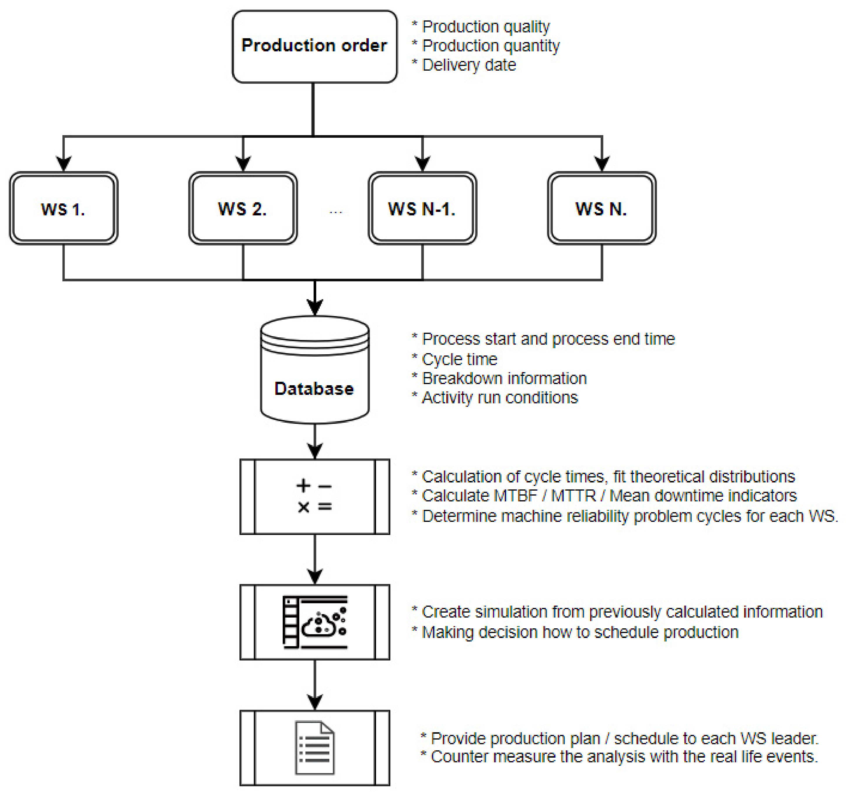
4.4.1. Optimization Method and Result

After analyzing the results from the simulation, real production scheduling is the focus. Since the company only had a cost calculation for production, our assumption is that cost differences of production are related to higher resource consumption. Nevertheless, regarding optimization, their objective was always minimizing certain KPIs.

To achieve a manageable mathematical model in size, daily capacities were implemented in the production scheduling method, which meant a daily scheduling program as a result. Since the cost implications for each simulation run had been calculated, the authors used average production cost figures per day. Besides this, since other costs can occur during production, another cost type, the inventory cost is built into the model. Based on lean principles, the company does not have to schedule its production to the earliest date possible because it is a waste. From the decision-maker's perspective, sometimes the safety of its service level is most important, and they would take extra costs just to keep the product in the inventory. It is up to the decision-maker; however, both these cases are discussed later.

As far as the optimization is concerned, the alternatives were the following:

• Producing on 1st/2nd/3rd/4th workshop on the 1st day (4 alternatives);
• Producing on 1st/2nd/3rd/4th workshop on the 2nd day (4 alternatives);
• Producing on 1st/2nd/3rd/4th workshop on the 3rd day (4 alternatives);
• Producing on 1st/2nd/3rd/4th workshop on the 4th day (4 alternatives);
• Producing on 1st/2nd/3rd/4th workshop on the 5th day (4 alternatives).

The model not only includes production, because additional alternatives such as inventory creation between days are added (four alternatives), since concluding from the results presented in the previous section, one day of production is not enough for fulfilling the customer need in terms of quantity.

The constraints of the model are acquired from the simulation and provided by the company: daily capacity per workshop is added (20 constraints), as well as demand information agreed (4 constraints). As per the orders, there is no continuous delivery, 100 pcs of product had to be delivered by the end of the week.

Constraints regarding capacity:

$$x_{ij}\le c_{ij}$$

(10)

$$i\in \left[1;4\right], j\in \left[1;5\right]$$

where

$x_{ij}$ represents production of a workshop $i$ on a certain day called $j$,

$c_{ij}$ represents capacity of a workshop $i$ on a certain day indicated $j$,

Constraints regarding demand in the first 4 days:

$${\displaystyle \sum }_{i=1}^4{\displaystyle \sum }_{j=1}^4{x}_{ij}\ge I_j$$

(11)

where

$x_{ij}$ represents production of a workshop $i$ on a certain day called $j$,

$I_j$ represents the demand of a certain day indicated $j \left(j\in \left[1;4\right]\right)$.

Based on the case study, the value for $I_j$ in the first 4 days is zero since the total amount of product should be delivered on the last day of production, in one batch.

Constraints regarding demand on the last day:

$${\displaystyle \sum }_{i=1}^4{x}_{i5}+T_4\ge I_5$$

(12)

where

$x_{ij}$ represents production of a workshop $i$ on the 5th day,

$T_4$ presents the accumulated inventory on the day 4.

$I_j$ indicates the demand on the last (5th) day.

As far as the last day’s constraint is concerned, the calculation can be the accumulated inventory on day 4th + 5th day of production from all workshops.

Two objectives were constructed and run during the optimization phase: first, the authors wanted to know how to schedule the production if they want to produce within the shortest time, and the second objective was the least total cost. In both cases, the same objective was applied (see Equation (13), but the variables had different values:

$$\min \mathrm{z}={\displaystyle \sum }_{i=1}^5{\displaystyle \sum }_{j=1}^5{c}_{ij}{x}_{ij}+{\displaystyle \sum }_{j=1}^4{T}_j\ast c^k$$

(13)

where,

${\displaystyle \sum }_{i=1}^5{\displaystyle \sum }_{j=1}^5{c}_{ij}{x}_{ij}$= total cost of workshop $j$ at a given day called $i$,

${\displaystyle \sum }_{j=1}^4{T}_j\ast c^k$ = Total inventory cost accumulated in the first 4 days.

When the earliest project finish was the objective, zero production cost, as well as a negative inventory cost (−0.001), was applied. That meant that all the capacities in the first couple of days per workshop would be utilized because in this case, the higher inventory volume can reduce cost. As a result, the following schedule was calculated, see

Table 7. Production schedule when production cost is not relevant.

	1st Day	2nd Day	3rd Day	4th Day	5th Day
Workshop 1.	5	6	5	5	6
Workshop 2.	6	5	6	6	5
Workshop 3.	6	5	6	5	0
Workshop 4.	6	6	5	6	0
Inventory	23	45	67	89	100

.

Because this production volume is a bit tight for the system, we can see that the company applied full capacity in the first 4 days, and the production pressure only went down on the last day of the working week. Having the sensitivity analysis investigated, it can be stated that based on the shadow price of the last day’s production, different production programs could also be assigned, and the objective value would not have changed. An important remark or limitation of the previous calculation is that this result is only available when the production-related costs are irrelevant.

The second scenario was about making cost figures relevant to see how the production schedule changes. As it was previously mentioned, daily operations costs were calculated by the division of production costs and number of products produced per day. This induces different cost figures over time, which—in real life—is also experienced by the companies.

Based on the inputs of the simulation, hourly production costs, raw material costs and reliability costs for two activities were implemented. The next step was to calculate the cost of producing 1 pc of product, which was followed by the calculation of the average production cost per day regarding workshops. The result of the calculation is displayed in the next table (see

Table 8. Production schedule when production cost is not relevant.

	1st Day	2nd Day	3rd Day	4th Day	5th Day
Workshop 1.	7,240.03	7,093.83	7,207.71	7,153.40	7,240.03
Workshop 2.	7,329.12	7,455.51	7,454.04	7,241.10	7,329.12
Workshop 3.	7,288.40	7,270.69	7,228.86	7,285.89	7,288.40
Workshop 4.	7,521.32	7,218.04	7,496.25	7,237.66	7,521.32
Inventory	350.00	350.00	350.00	350.00	350.00

). The values are given in universal metrics, so-called CU—currency unit in favor of the company.

These figures were applied in the optimization model. Having the inventory cost included, it can be clearly seen that the vast majority of the serial production should be performed later in the time period. As a result of the optimization, the following schedule would be optimal, see

Table 9. Production schedule when production cost is a relevant decision variable.

	1st Day	2nd Day	3rd Day	4th Day	5th Day
Workshop 1.	0	6	5	5	6
Workshop 2.	6	5	6	6	6
Workshop 3.	0	5	6	5	7
Workshop 4.	3	6	5	6	6
Inventory	9	31	53	75	100

.

The beginning of the week dedicated to this production can be used by finishing the previous projects; additionally, productive maintenance would be performed or assigned as buffer time. As far as the total cost is concerned, 788 281.02 CU (currency unit) would be the cost of creating 100 pcs of product, when the optimal cost is the objective.

When the supply safety (use the full capacity at the beginning of the week and keep higher inventory until the end of the period) is the priority, the cost would be slightly higher (up to 17 823.91, which is ~2.26%) to realize 806 104.93 CU as a cost value. If this cost reduction possibility is utilized, it is essential to pay enough attention to improvement possibilities.

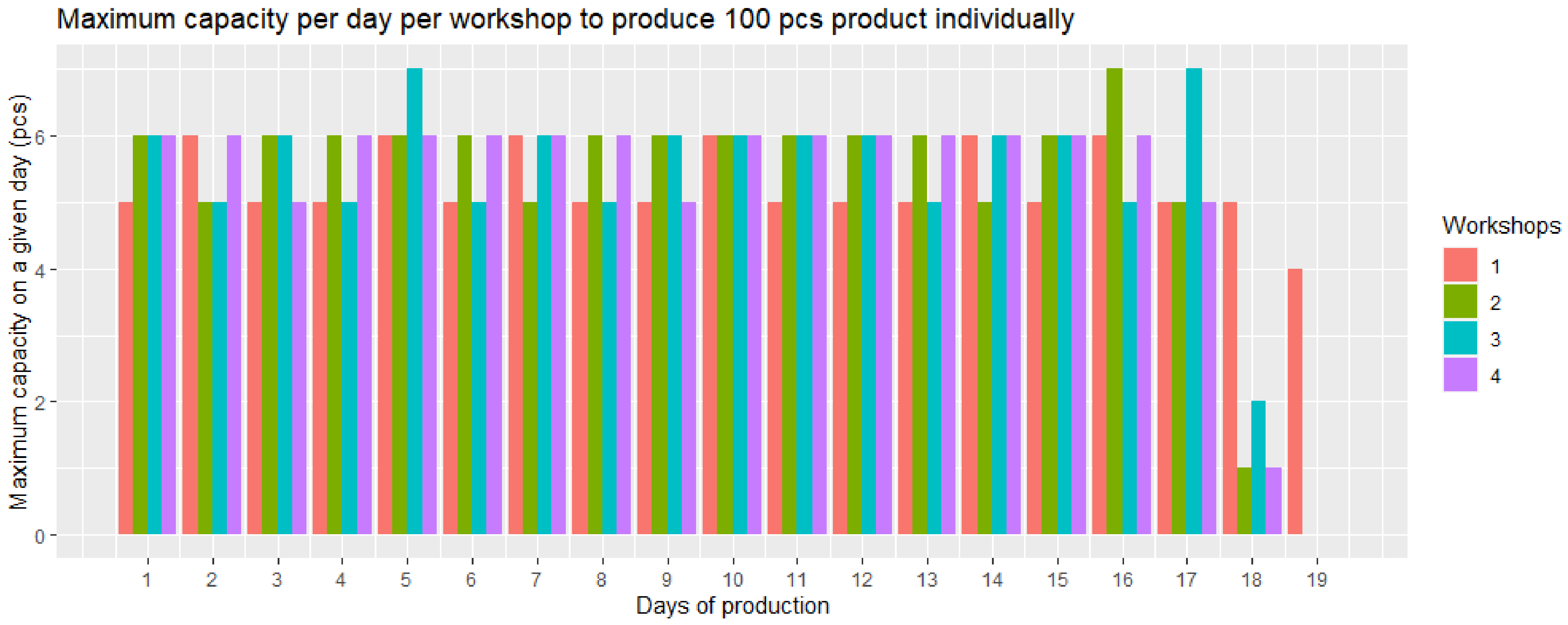
4.4.2. Additional Analyses without Cost Calculations

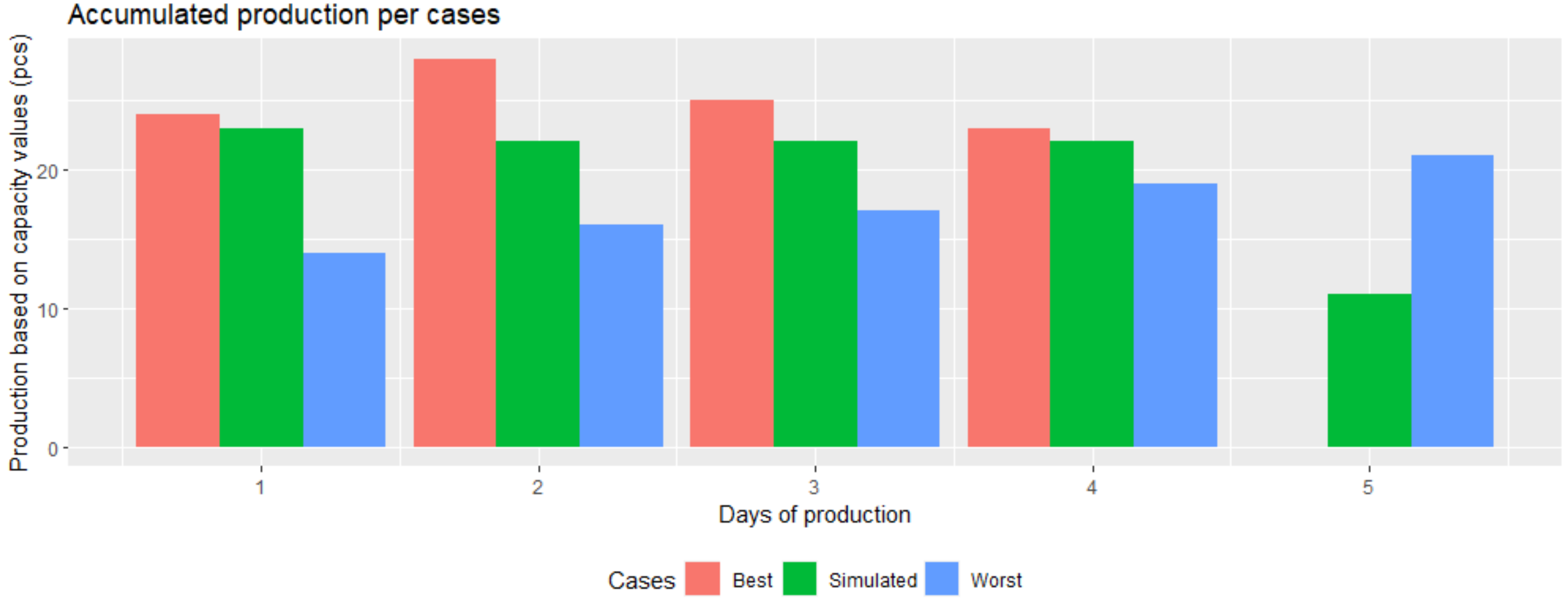
Complementary to this analysis, the worst and best cases were also analyzed where the least and most capacity days were implemented in the optimization model. As the diagram shows below (Figure 6), in the best-case scenario, there is no need for production on the last day (fifth), additionally, in the worst-case plan, it is impossible to produce the required amount of product.

From the manufactured product it is easy to calculate the inventory per day per scenario indicator. Based on the table below, it can be inferred from the values that in the worst-case scenario the kept stock and the inventory cost are smaller, but this is because in this case the workshops are not able to produce 100 pcs of product in a given week (see

Table 10. Inventory values per scenario.

	1st Day	2nd Day	3rd Day	4th Day	5th Day
As-is case based on simulation	23	45	67	89	100
Best case based on simulation	24	52	77	100	100
Worst case based on simulation	14	30	47	66	87

).

This case can be also considered when there is a negotiation about the time or the produced volume. Alternatively, when the best case is under investigation, it can be seen that there is no need for the last day, another project or serial production can use this slack time/time puffer. This can make the company feeling comfortable which can compensate for the tight schedule provided by the optimization.

This complementary analysis is for investigating all the possible opportunities to have a full picture of the possible outcomes. As the last step of the decision-preparation period, the decision-maker has to decide based on his/her risk tolerance level. In most cases (2/3 cases), the deadline can be easily kept, which means that no penalty has to be paid because of overdue production on the one hand. On the other hand, the company’s reputation can also be lifted due to the on-time delivery, which is a crucial part of satisfying customers. In the worst-case scenario, all the problems occur during the production at each workshop, which is not likely; however, this also has to be taken into account in order to provide the broadest information for managers. Based on this, and other negotiated values (such as penalty and deadline), the company can determine if the project is worthy or not, or what kind of workaround has to be made in order to reduce the probability of the problems or increase efficiency—for example, buying or renting other, more reliable machines for production. This can modify the cost and the selling price, but this is also a valuable contribution—and another perspective to investigate possible risks during production.

5. Discussion

One of the main ideas of lean manufacturing is to decrease the applied resources to a level with which the company can fulfill customer demand [1]. This system requires well-thought-out planning of the product itself, the entire production process, as well as the assignment of work for different workshops. This ability is valued when a unique product is designed and produced. The main focus point of the research was to implement reliability indicators in a stochastic environment since there is a literature gap in this field, and the Monte-Carlo simulation is frequently used for simulating stochastic process steps. The developed framework carries through the reader the main milestones of the reliability indicator-based (or risk-adjusted) production scheduling: what to measure, how to measure, and how to use and synthesize the gathered information to achieve the best result. The main barrier during the application of the method is the reliability and availability of the data necessary, but the process can be effectively applied under the Industry 4.0 domain, where MES supports the decision-maker's work [18,19].

This paper presents a case study where workshops produce the same product in smaller quantities (100 pieces), but with slight differences: different machines and human resources for different workshops, and due to these changes, with different reliability values. The implementation of reliability-based indicators to the Stochastic CPM method considering one workshop was discussed earlier in an article [41], and that method was complemented with a production scheduling approach, which is a critical point when more than one unit produces the product. For this, a linear programming optimization method has been applied to the cost of production as well as the cost of inventory holding. Another merit of the presented result is that the decision-maker will be able to estimate the time frame necessary to conduct a project with higher confidence and with a smaller margin of error, which can result in more satisfying customers. The scheduling will also be traceable and trackable due to real-time data.

A detailed analysis was provided in this article regarding stochastic cycle times and total costs, but as a future research direction, more-in-detail analysis can be made from the company’s controlling perspective. Additionally, in an investigation of a complex environment, in which many workshop works and products are produced, planning for the entire year can be also achieved, where projects are prioritized every time a new work order or request for proposal is placed. As another research direction, the automation of the presented framework can also be executed, which synthesizes every process run at each workshop, and the information about the production can be used for the planning of the remaining quantities’ production. This would serve more accurate planning and flexibility from the production point of view.

6. Conclusions

In this paper, a combination of a modified stochastic critical path method and a production scheduling method was presented through a case report. The focus point of the research was a serial production carried out by four workshops, who are performing their work based on project manufacturing principles. The objective under investigation was the minimization of cost since many, non-value-added activities not only consume natural or not natural resources, but they can also have a great influence on the cost figures as well. The model was complemented with information about machine reliability—mean time between failure given in the cycle of machine use, and total downtime, which displays the time effort repairing the machine to continue production.

Research hypotheses were tested, and case presentation supported the answer: when process activity times are measured, a more detailed analysis can be made, since more points can be gathered from an activity than before. The collected time values can support analysts to fit the theoretical distribution to the activities. Other information regarding machine reliability can also provide reinforcement for the simulation and forecasting of production. All the information served as input for the framework that includes process time prediction and production scheduling as well considering capacity restrictions. The production scheduling was conducted with the use of linear programming with transfer variables, which were responsible to indicate inventory level. Two scenarios of production scheduling were also created: one with inventory cost, and one without inventory cost. The result of the distinguished objective functions was different, which highlighted two different production strategies. Such information plays a crucial role in the initial negotiations for the contracting with the customer since a more realistic deadline can be set up due to the integration of possible risks in the production. Another workaround can also be invented in order to avoid risks or decrease the probability of occurrence indicator. Additionally, cost implications can be calculated.

As the case report demonstrates, the company would be able to finish within the predetermined time period (5 working days), as well as extra resources were available in case of delayed production. Planning by the presented risk-adjusted production scheduling at workshop layout manufacturing process can ensure the company sees their resources, costs and capacities clearly, which can be a huge advantage on the market, and it can support well-thought-out deliveries, and other, either value-added or non-value-added activities. It is important to highlight that the simulation was performed for the “as-is” situation, which means that no improvement took place during the analysis. Based on lean principles and many other production strategies, continuous improvement for a reduction in uncertainty in production should be one of the focus areas.

References

1. Womack, J.P.; Jones, D.T. Lean Thinking: Banish Waste and Create Wealth in Your Corporation; Free Press: New York, NY, USA, 2003. [Google Scholar]
2. Womack, J.P.; Jones, D.T. The Machine That Changed the World: The Story of Lean Production; Free Press: New York, NY, USA, 1990. [Google Scholar]
3. Poswa, F.; Adenuga, O.T.; Mpofu, K. Productivity Improvement Using Simulated Value Stream Mapping: A Case Study of the Truck Manufacturing Industry. Processes 2022, 10, 1884. [Google Scholar] [CrossRef]
4. Garcia-Garcia, G.; Singh, Y.; Jagtap, S. Optimising Changeover through Lean-Manufacturing Principles: A Case Study in a Food Factory. Sustainability 2022, 14, 8279. [Google Scholar] [CrossRef]
5. Kunkera, Z.; Tošanović, N.; Štefanić, N. Improving the Shipbuilding Sales Process by Selected Lean Management Tool. Machines 2022, 10, 766. [Google Scholar] [CrossRef]
6. Wang, C.-N.; Huang, Y.-F.; Le, T.-N.; Ta, T.-T. An Innovative Approach to Enhancing the Sustainable Development of Japanese Automobile Suppliers. Sustainability 2016, 8, 420. [Google Scholar] [CrossRef] [Green Version]
7. Milewski, D. Managerial and Economical Aspects of the Just-In-Time System “Lean Management in the Time of Pandemic”. Sustainability 2022, 14, 1204. [Google Scholar] [CrossRef]
8. Peron, M.; Fragapane, G.; Sgarbossa, F.; Kay, M. Digital Facility Layout Planning. Sustainability 2020, 12, 3349. [Google Scholar] [CrossRef] [Green Version]
9. Siva, R.; Prabakaran, M.; Rishikesh, S.; Santhosh Kumar, A.; Sangeetha, M. Lead time reduction through lean techniques on filter drier component by modifying fixture design—Case study. Mater. Today Proc. 2020, 33, 2651–2655. [Google Scholar] [CrossRef]
10. Naciri, L.; Mouhib, Z.; Gallab, M.; Nali, M.; Abbou, R.; Kebe, A. Lean and industry 4.0: A leading harmony. Procedia Comput. Sci. 2022, 200, 394–406. [Google Scholar] [CrossRef]
11. Tortorella, G.L.; Fettermann, D. Implementation of Industry 4.0 and lean production in Brazilian manufacturing companies. Int. J. Prod. Res. 2017, 56, 2975–2987. [Google Scholar] [CrossRef]
12. Mayer, L.; Mehdiyev, N.; Fettke, P. Manufacturing execution systems driven process analytics: A case study from individual manufacturing. Procedia CIRP 2021, 97, 284–289. [Google Scholar] [CrossRef]
13. Jaskó, S.; Skrop, A.; Holczinger, T.; Chován, T.; Abonyi, J. Development of manufacturing execution systems in accordance with Industry 4.0 requirements: A review of standard- and ontology-based methodologies and tools. Comput. Ind. 2020, 123, 103300. [Google Scholar] [CrossRef]
14. Itskovich, E.L. Fundamentals of Design and Operation of Manufacturing Executive Systems (MES) in Large Plants. IFAC Proc. Vol. 2013, 46, 313–318. [Google Scholar] [CrossRef]
15. Tian, X.; Xie, J.; Xu, M.; Wang, Y.; Liu, Y. An infinite life cycle assessment model to re-evaluate resource efficiency and environmental impacts of circular economy systems. Waste Manag. 2022, 145, 72–82. [Google Scholar] [CrossRef]
16. Venkatraj, V.; Dixit, M.K. Challenges in implementing data-driven approaches for building life cycle energy assessment: A review. Renew. Sustain. Energy Rev. 2022, 160, 112327. [Google Scholar] [CrossRef]
17. Dutta, G.; Kumar, R.; Sindhwani, R.; Singh, R.K. Overcoming the barriers of effective implementation of manufacturing execution system in pursuit of smart manufacturing in SMEs. Procedia Comput. Sci. 2022, 200, 820–832. [Google Scholar] [CrossRef]
18. Chohan, B.S.; Xu, X.; Lu, Y. MES Dynamic interoperability for SMEs in the Factory of the Future perspective. Procedia CIRP 2022, 107, 1329–1335. [Google Scholar] [CrossRef]
19. Perico, P.; Arica, E.; Powell, D.J.; Gaiardelli, P. MES as an Enabler of Lean Manufacturing. IFAC-PapersOnLine 2019, 52, 48–53. [Google Scholar] [CrossRef]
20. Widiasih, W.; Karningsih, P.D.; Ciptomulyono, U. Development of Integrated Model for Managing Risk in Lean Manufacturing Implementation: A Case Study in an Indonesian Manufacturing Company. Procedia Manuf. 2015, 4, 282–290. [Google Scholar] [CrossRef] [Green Version]
21. Chi, C.F.; Sigmund, D.; Astardi, M.O. Classification Scheme for Root Cause and Failure Modes and Effects Analysis (FMEA) of Passenger Vehicle Recalls. Reliab. Eng. Syst. Saf. 2020, 200, 106929. [Google Scholar] [CrossRef]
22. Barghi, B.; Shadrokh sikari, S. Qualitative and quantitative project risk assessment using a hybrid PMBOK model developed under uncertainty conditions. Heliyon 2020, 6, e03097. [Google Scholar] [CrossRef]
23. Ok, C.I.; Kim, C.L.; Moon, S.R.; Koo, H.S.; Yun, K.H.; Lee, S.K. Prioritization of radiological accident scenarios during decommissioning of nuclear power plants by risk matrix and AHP method. Ann. Nucl. Energy 2022, 175, 109239. [Google Scholar] [CrossRef]
24. Ouyang, L.; Che, Y.; Yan, L.; Park, C. Multiple perspectives on analyzing risk factors in FMEA. Comput. Ind. 2022, 141, 103712. [Google Scholar] [CrossRef]
25. Rhee, S.J.; Ishii, K. Using cost based FMEA to enhance reliability and serviceability. Adv. Eng. Inform. 2003, 17, 179–188. [Google Scholar] [CrossRef]
26. Kocsi, B.; Matonya, M.M.; Pusztai, L.P.; Budai, I. Real-Time Decision-Support System for High-Mix Low-Volume Production Scheduling in Industry 4.0. Processes 2020, 8, 912. [Google Scholar] [CrossRef]
27. Li, C.; Chen, Y.; Shang, Y. A review of industrial big data for decision making in intelligent manufacturing. Eng. Sci. Technol. Int. J. 2021, 29, 101021. [Google Scholar] [CrossRef]
28. Seibold, J.; Hentsch, M.; Kharitonov, A.; Eber, R.; Schwarzer, S. Process automation in the area of manufacturability analysis using machine learning. Procedia Comput. Sci. 2022, 204, 196–204. [Google Scholar] [CrossRef]
29. Mossa, G.; Boenzi, F.; Digiesi, S.; Mummolo, G.; Romano, V.A. Productivity and ergonomic risk in human based production systems: A job-rotation scheduling model. Int. J. Prod. Econ. 2016, 171, 471–477. [Google Scholar] [CrossRef]
30. Li, C.Z.; Shen, G.Q.; Xu, X.; Xue, F.; Sommer, L.; Luo, L. Schedule risk modeling in prefabrication housing production. J. Clean. Prod. 2017, 153, 692–706. [Google Scholar] [CrossRef]
31. Zareei, S. Project scheduling for constructing biogas plant using critical path method. Renew. Sustain. Energy Rev. 2018, 81, 756–759. [Google Scholar] [CrossRef]
32. Trevino-Martinez, S.; Sawhney, R.; Shylo, O. Energy-carbon footprint optimization in sequence-dependent production scheduling. Appl. Energy 2022, 315, 118949. [Google Scholar] [CrossRef]
33. Wayne, L. Winston. Operations Research; Thomson Learning: Belmont, CA, USA, 2004. [Google Scholar]
34. Ragsdale, C. Spreadsheet Modeling & Decision Analysis: A Practical Introduction to Business Analytics; Cengage Learning: Boston, MA, USA, 2017. [Google Scholar]
35. Temesi, J.; Varró, Z. Operációkutatás; Akadémiai Kiadó: Budapest, Hungary, 2014. [Google Scholar]
36. Schweickert, R. Constructing a stochastic critical path network given the slacks: Representation. Math. Soc. Sci. 1992, 23, 343–366. [Google Scholar] [CrossRef]
37. Takakura, Y.; Yajima, T.; Kawajiri, Y.; Hashizume, S. Application of critical path method to stochastic processes with historical operation data. Chem. Eng. Res. Des. 2019, 149, 195–208. [Google Scholar] [CrossRef]
38. Badiru, A.B. A simulation approach to PERT network analysis. Simulation 1991, 57, 245–255. [Google Scholar] [CrossRef] [Green Version]
39. Wilmott, P.; McCarthy, D. TPM—A Route to World Class Performance; Elsevier: Amsterdam, The Netherlands, 2000. [Google Scholar]
40. Brunelli, L.; Masiero, C.; Tosato, D.; Beghi, A.; Susto, G.A. Deep Learning-based Production Forecasting in Manufacturing: A Packaging Equipment Case Study. Procedia Manuf. 2019, 38, 248–255. [Google Scholar] [CrossRef]
41. Pusztai, L.P.; Nagy, L.; Budai, I. Selection of Production Reliability Indicators for Project Simulation Model. Appl. Sci. 2022, 12, 5012. [Google Scholar] [CrossRef]
Figure 1. Conceptual framework for quantitative risk analysis-based production scheduling.
Sustainability 15 01395 g001
Figure 2. AOA Process representation for the workshops. Arrows represent activities, nodes represent events.
Sustainability 15 01395 g002
Figure 3. Performance of the workshops compared to the Takt Time.
Sustainability 15 01395 g003
Figure 4. Box plot of the total process times per workshop.
Sustainability 15 01395 g004
Figure 5. Daily capacity per workshop.
Sustainability 15 01395 g005
Figure 6. Daily production for all scenarios.
Sustainability 15 01395 g006