


A Comparison between Supervised Classification Methods: Study Case on Land Cover Change Detection Caused by a Hydroelectric Complex Installation in the Brazilian Amazon

 ,
,  ,
,  , , and
Abstract
1. Introduction
2. Materials and Methods
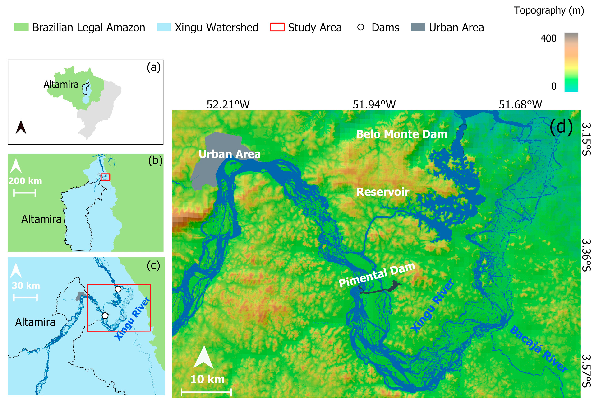
2.1. Study Area
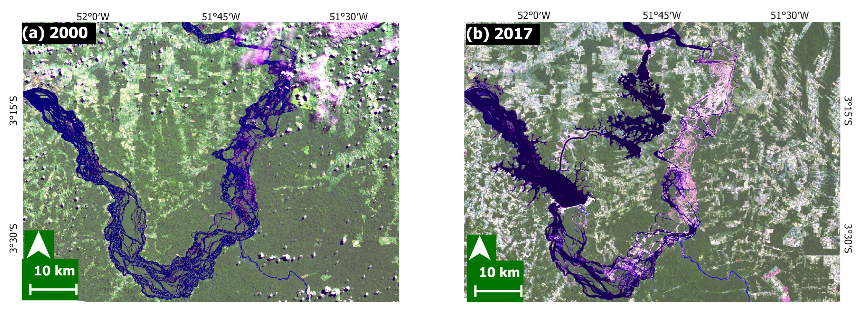
2.2. Dataset

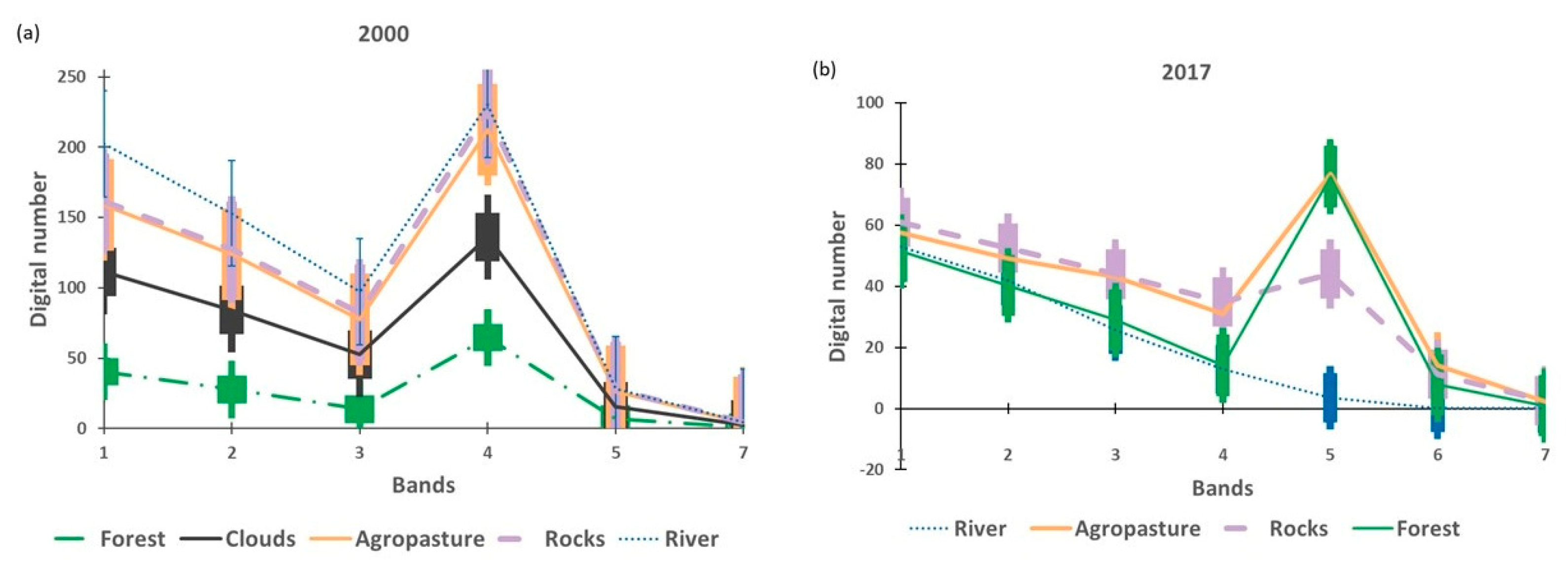
2.3. Class Selection and Spectral Signatures
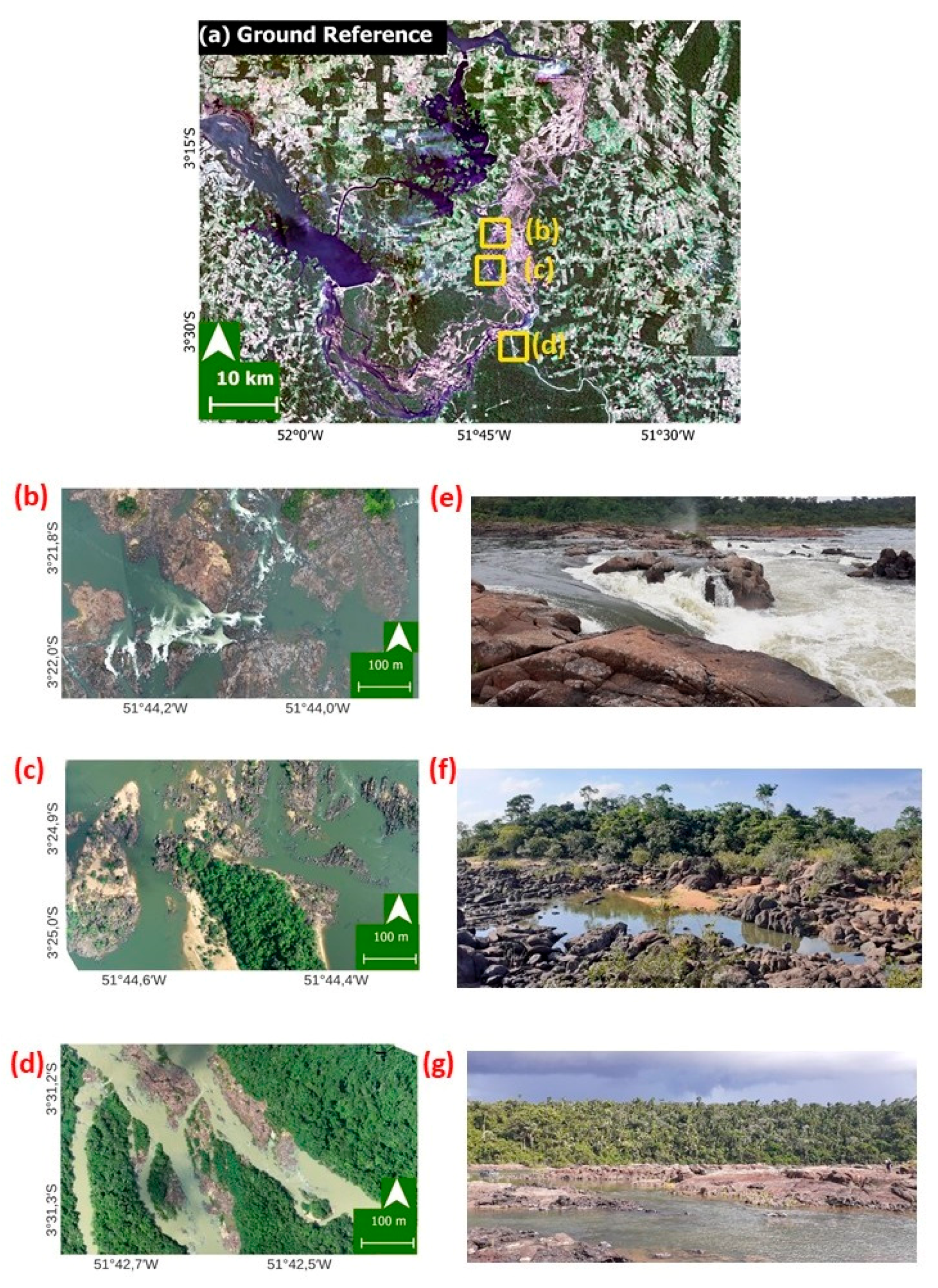
2.4. Reference Data

2.5. Complementary Data
2.6. Image Classification
2.7. Accuracy Assessment
- Overall Accuracy (OA): calculated by summing the number of reliable classified pixels divided by the total number of training pixels.
- Errors of Commission (Comm): are the fraction of sample pixels that were predicted to be in a class but do not belong to that class (false positives).
- Errors of Omission (Om): are the fraction of pixels that belong to a class but were predicted to be in a different class (false negatives).
- Producer Accuracy (PA): a measure of the probability that a pixel in a given class was classified properly.
- User Accuracy (UA): a measure of the probability that a pixel predicted to be in a certain class really belongs to that class.
- Kappa Coefficient (Kappa): takes non-diagonal elements into account and measures how equivalent classification and reference values are. A kappa value of 1 represents a perfect match, while a value of 0 represents no equivalence. Despite the criticism by some authors, the kappa coefficient is considered a powerful tool when analyzing a single error matrix and for comparing the differences between various error matrices [43,60].
2.8. Detecting Land Cover Change
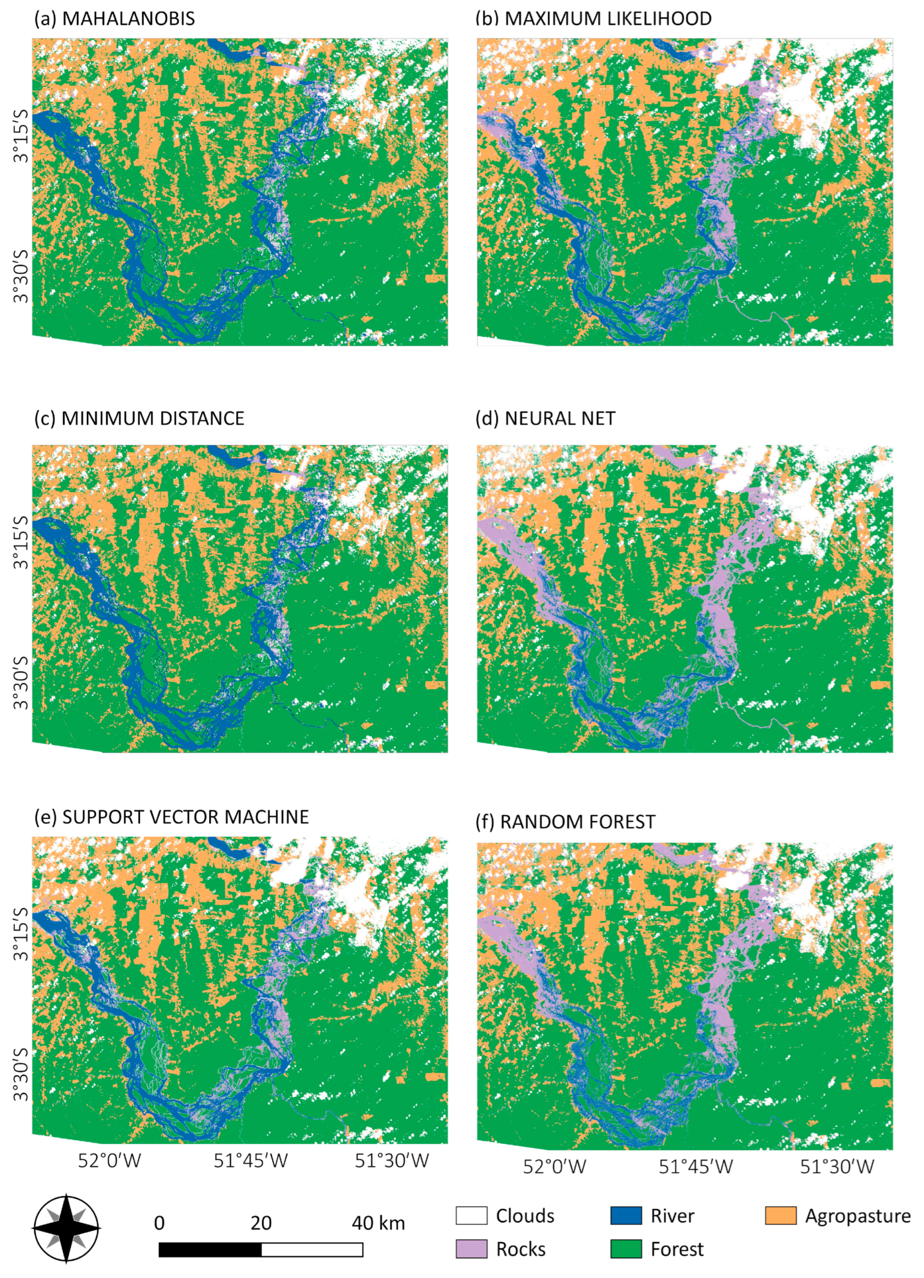
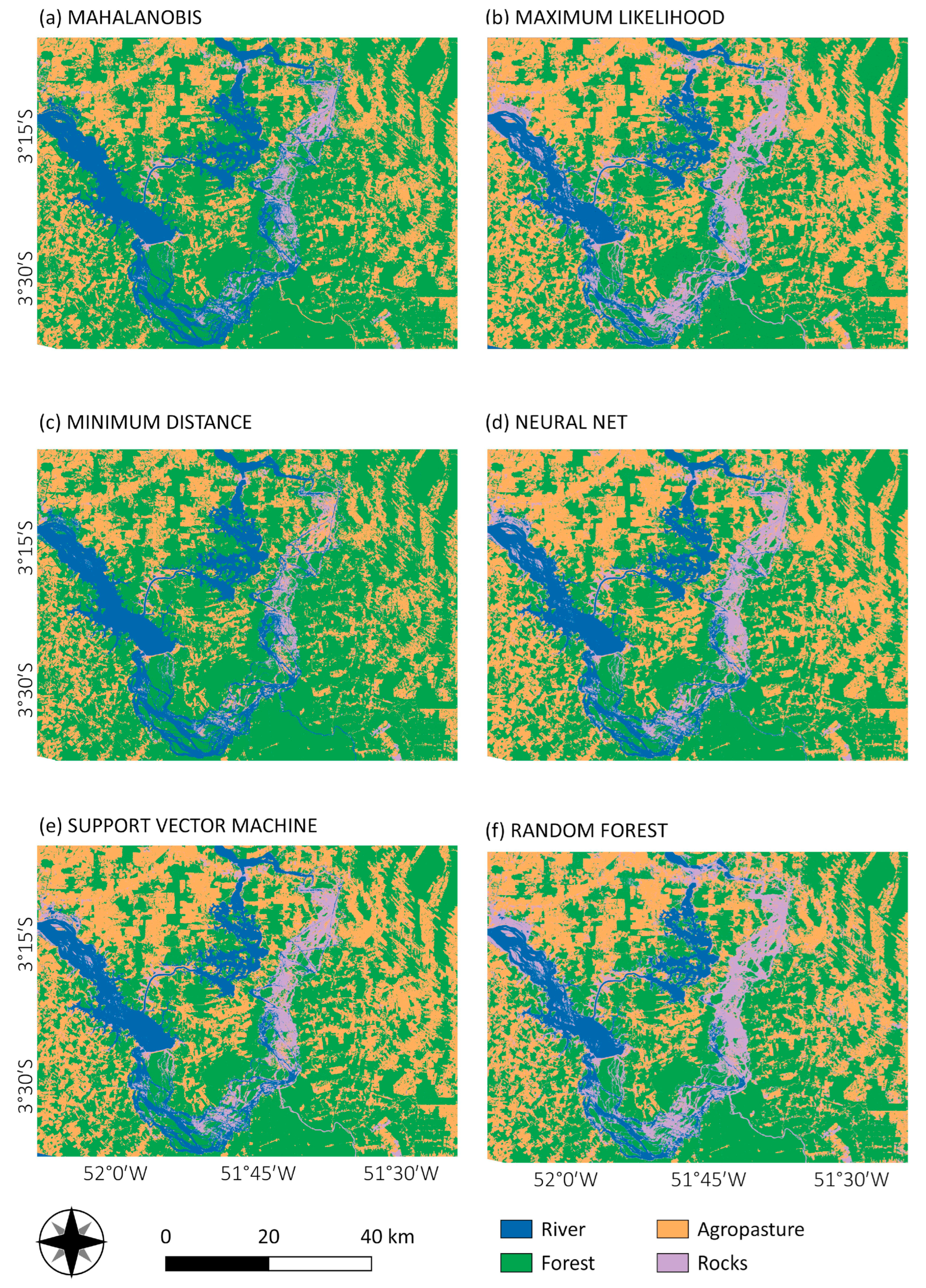
3. Results
3.1. Classification Accuracy Assessment
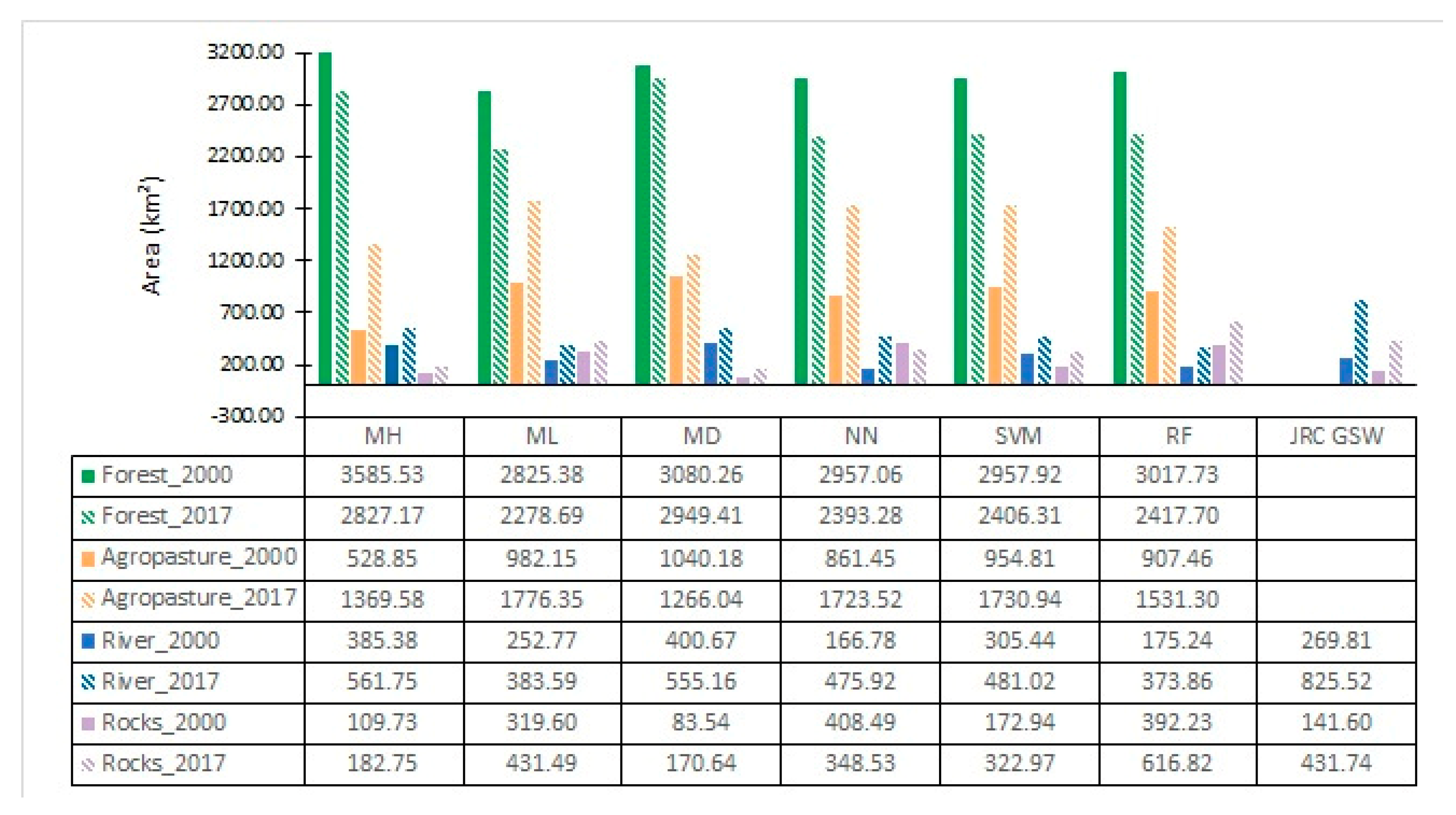
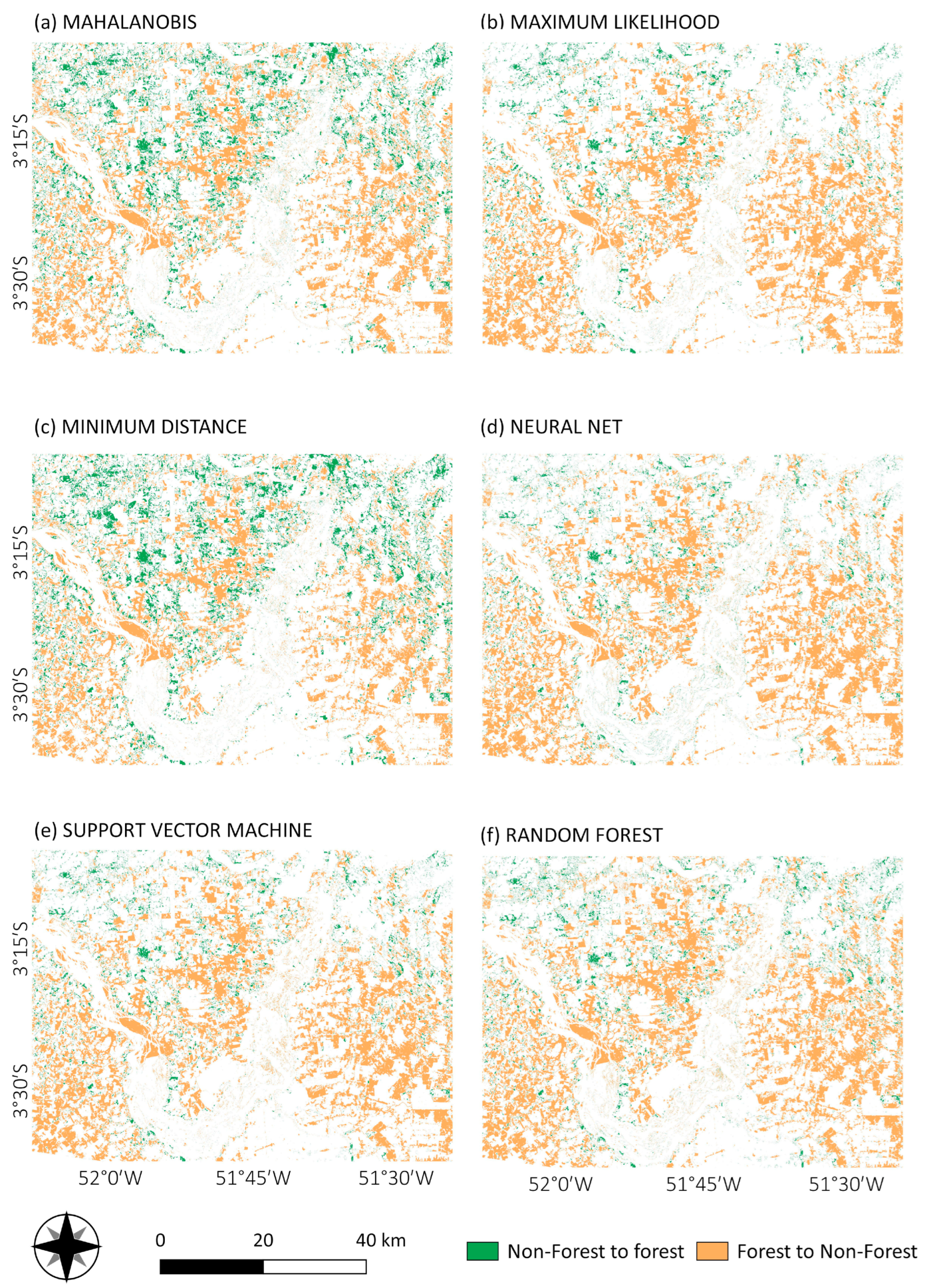
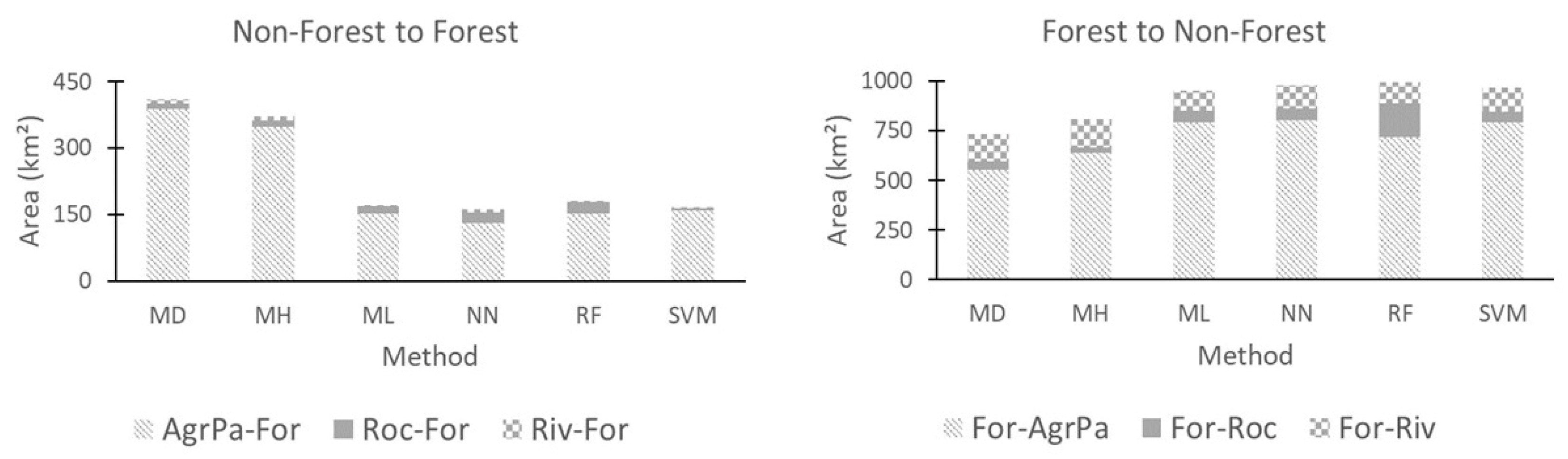
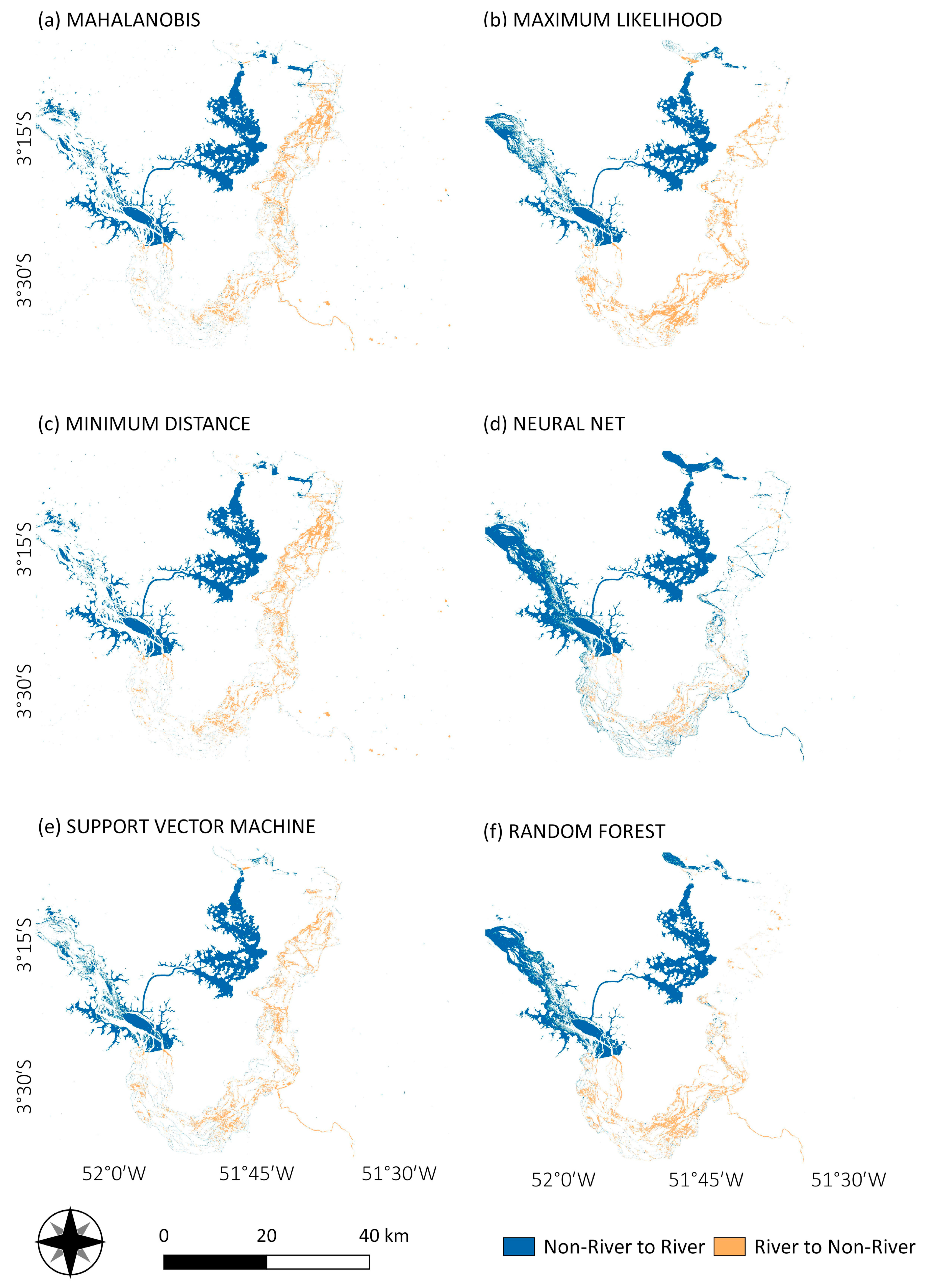
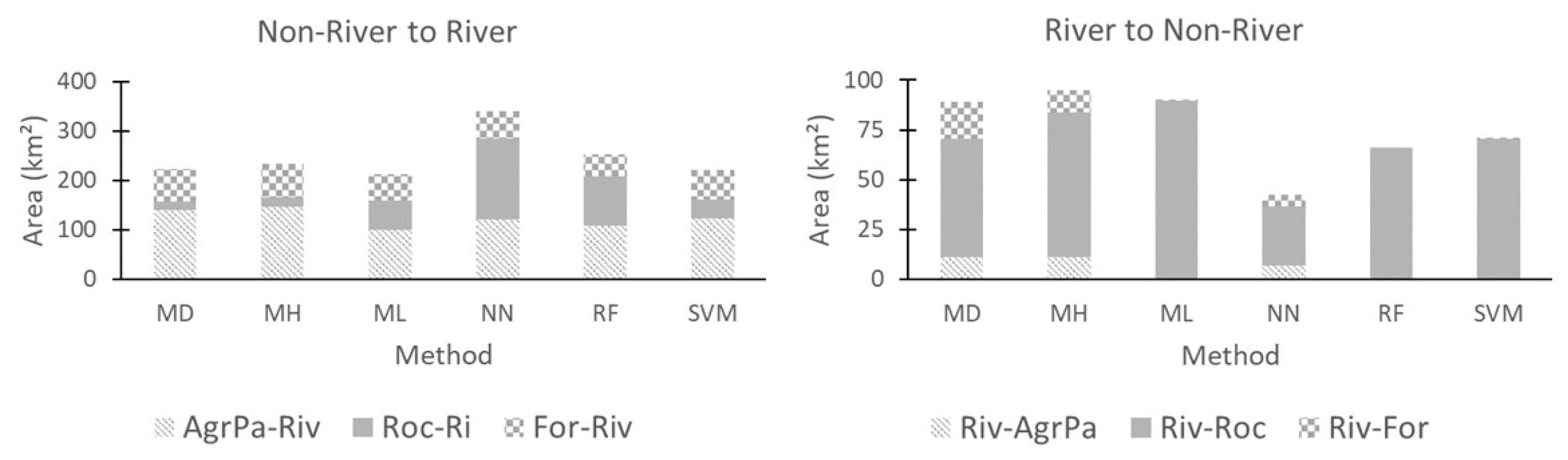
3.2. Land Cover Change
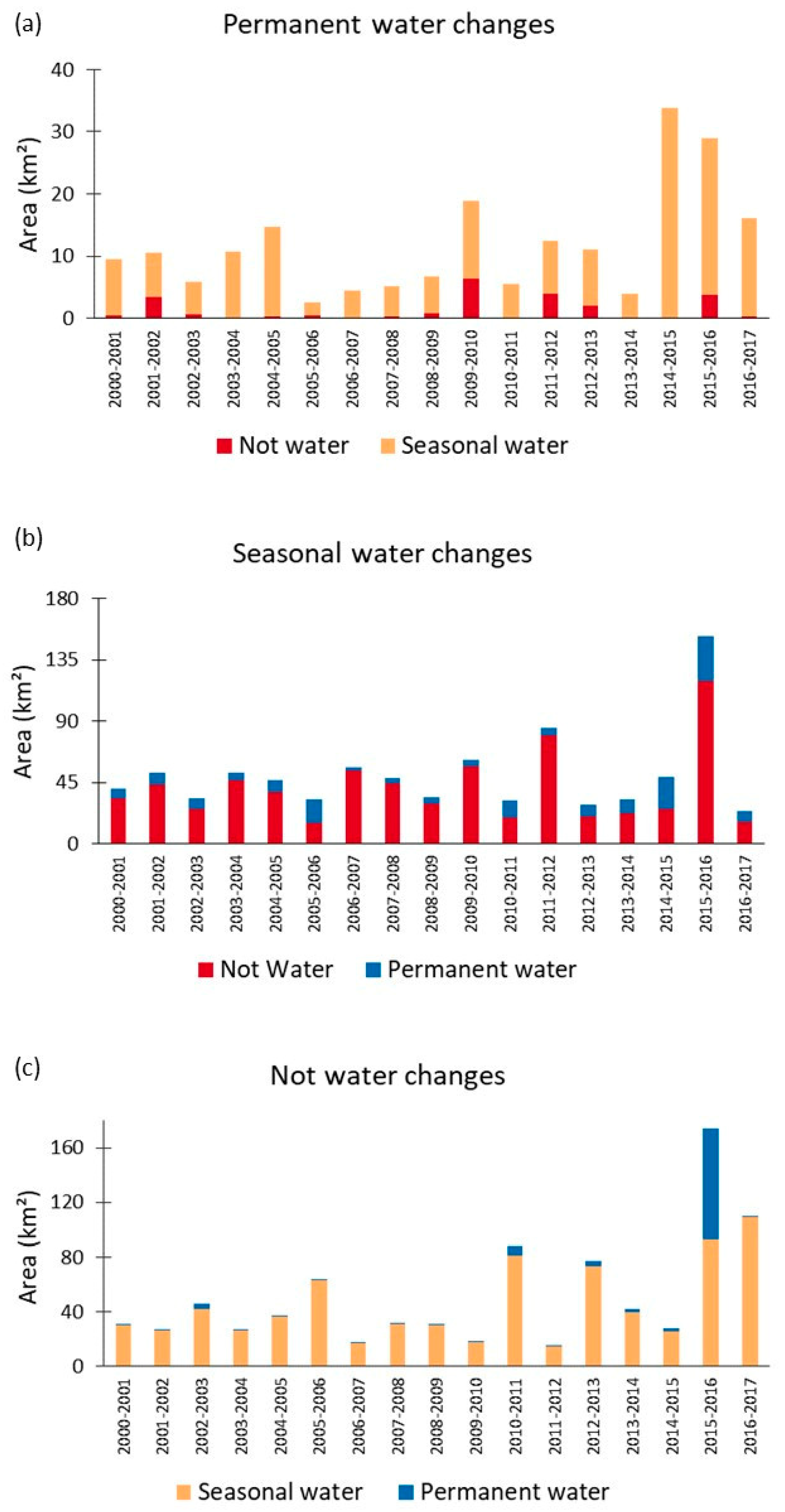
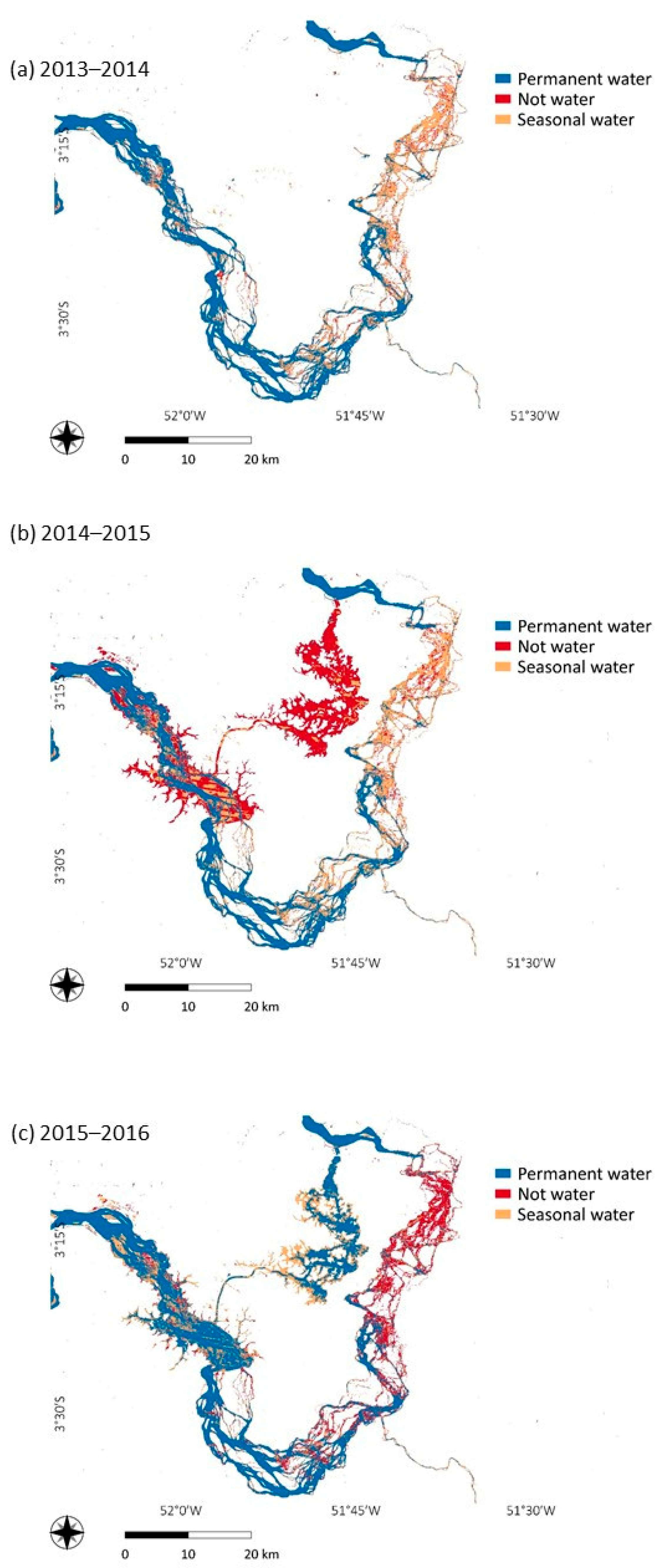
3.3. JRC Ground Surface Water Dataset
4. Discussion
4.1. Accuracy Assessment of Classification Methods
4.2. Land Use and Land Cover Changes
5. Conclusions
Author Contributions
Funding
Data Availability Statement
Acknowledgments
Conflicts of Interest
References
- Skole, D.L.; Chomentowski, W.; Salas, W.; Nobre, A.D. Physical and Human Dimensions of Deforestation in Amazonia. BioScience 1994, 44, 314–322. [Google Scholar] [CrossRef]
- de Mello, K.; Valente, R.A.; Randhir, O.T.; Santos, A.C.; Vettorazzi, C.A. Effects of Land Use and Land Cover on Water Quality of Low-Order Streams in Southeastern Brazil: Watershed Versus Riparian Zone. CATENA 2018, 167, 130–138. [Google Scholar] [CrossRef]
- Kalacska, M.; Arroyo-Mora, J.; Lucanus, O.; Sousa, L.; Pereira, T.; Vieira, T. Deciphering the Many Maps of the Xingu—An Assessment of Land Cover Classifications at Multiple Scales. Proc. Acad. Nat. Sci. Phila. 2020, 166, 1–55. [Google Scholar] [CrossRef]
- Rosa, I.M.; Gabriel, C.; Carreiras, J.M. Spatial and Temporal Dimensions of Landscape Fragmentation across the Brazilian Amazon. Reg. Environ. Chang. 2017, 17, 1687–1699. [Google Scholar] [CrossRef]
- Moretto, E.M.; Gomes, C.S.; Roquetti, D.R.; Jordão, C.D.O. Histórico, Tendências e Perspectivas no planejamento espacial de Usinas Hidrelétricas Brasileiras: A Antiga e Atual Fronteira Amazônica. Ambiente Soc. 2012, 15, 141–164. [Google Scholar] [CrossRef]
- Fearnside, P.M. Hidrelétricas Na Amazônia: Impactos Ambientais e Sociais Na Tomada De Decisões Sobre Grandes Obras; Editora do INPA: Belém, Brazil, 2015; Volume 2, p. 2. [Google Scholar]
- Athayde, S.; Duarte, C.G.; Gallardo, A.L.; Moretto, E.M.; Sangoi, L.A.; Dibo, A.P.A.; Siqueira-Gay, J.; Sánchez, L.E. Improving Policies and Instruments to Address Cumulative Impacts of Small Hydropower in the Amazon. Energy Policy 2019, 132, 265–271. [Google Scholar] [CrossRef]
- Marengo, J.A.; Souza, C.A.J.; Thonicke, K.; Burton, C.; Halladay, K.; Betts, R.A.; Alves, L.M.; Soares, W.R. Changes in climate and land use over the Amazon region: Current and future variability and Trends. Front. Earth Sci. 2018, 6, 135. [Google Scholar] [CrossRef]
- Farinosi, F.; Arias, M.E.; Lee, E.; Longo, M.; Pereira, F.; Livino, A.; Moorcroft, P.R.; Briscoe, J. Future climate and land use change impacts on river flows in the tapajós basin in the Brazilian Amazon. Earth’s Future 2019, 7, 993–1017. [Google Scholar] [CrossRef]
- Arias, M.E.; Farinosi, F.; Lee, E.; Livino, A.; Briscoe, J.; Moorcroft, P.R. Impacts of climate change and deforestation on hydropower planning in the Brazilian Amazon. Nat. Sustain. 2020, 3, 430–436. [Google Scholar] [CrossRef]
- Winemiller, K.O.; McIntyre, P.B.; Castello, L.; Fluet-Chouinard, E.; Giarizzp, T.; Nam, S.; Saénz, L. Balancing hydropower and biodiversity in the Amazon, Congo, and Mekong. Science 2016, 351, 128–129. [Google Scholar] [CrossRef]
- Jiang, X.; Lu, D.; Moran, E.; Calvi, M.F.; Dutra, L.V.; Li, G. Examining Impacts of the Belo Monte Hydroelectric Dam Construction on Land-Cover Changes Using Multitemporal Landsat Imagery. Appl. Geogr. 2018, 97, 35–47. [Google Scholar] [CrossRef]
- Calvi, M.F.; Moran, E.F.; da Silva, R.F.B.; Batistella, M. The Construction of the Belo Monte Dam in the Brazilian Amazon and Its Consequences on Regional Rural Labor. Land Use Policy 2020, 90, 104327. [Google Scholar] [CrossRef]
- Swanson, A.C.; Bohlman, S. Cumulative Impacts of Land Cover Change and Dams on the Land–Water Interface of the Tocantins River. Front. Environ. Sci. 2021, 9, 662904. [Google Scholar] [CrossRef]
- Li, G.; Lu, D.; Moran, E.; Hetrick, S. Land-Cover Classification in a Moist Tropical Region of Brazil with Landsat Thematic Mapper Imagery. Int. J. Remote Sens. 2011, 32, 8207–8230. [Google Scholar] [CrossRef] [PubMed]
- Singh, A. Review Article Digital Change Detection Techniques Using Remotely-Sensed Data. Int. J. Remote Sens. 1989, 10, 989–1003. [Google Scholar] [CrossRef]
- Lu, D.; Weng, Q. A Survey of Image Classification Methods and Techniques for Improving Classification Performance. Int. J. Remote Sens. 2007, 28, 823–870. [Google Scholar] [CrossRef]
- Lu, D.; Mausel, P.; Batistella, M.; Moran, E. Comparison of Land-Cover Classification Methods in the Brazilian Amazon Basin. Photogramm. Eng. Remote Sens. 2004, 70, 723–731. [Google Scholar] [CrossRef]
- Lefsky, M.A.; Cohen, W.B. Selection of Remotely Sensed Data. In Remote Sensing of Forest Environments: Concepts and Case Studies; Essay; Kluwer Academic Publishers: Boston, MA, USA, 2003; pp. 13–46. [Google Scholar]
- Zhu, Z. Change Detection Using Landsat Time Series: A Review of Frequencies, Preprocessing, Algorithms, and Applications. ISPRS J. Photogramm. Remote Sens. 2017, 130, 370–384. [Google Scholar] [CrossRef]
- Asner, G.P. Cloud cover in landsat observations of the Brazilian Amazon. Int. J. Remote Sens. 2001, 22, 3855–3862. [Google Scholar] [CrossRef]
- Souza, C.M.; Shimbo, J.Z.; Rosa, M.R.; Parente, L.L.; Alencar, A.; Rudorff, B.F.; Hasenack, H.; Matsumoto, M.; Ferreira, L.G.; Souza-Filho, P.W.E. Reconstructing three decades of land use and land cover changes in Brazilian biomes with Landsat Archive and Earth engine. Remote Sens. 2020, 12, 2735. [Google Scholar] [CrossRef]
- Michael, G.; Barthem, R.; Ferreira, E.J.G.; Duenas, R. The Smithsonian Atlas of the Amazon; Smithsonian Books: Washington, DC, USA, 2010. [Google Scholar]
- Barona, E.; Ramankutty, N.; Hyman, G.; Coomes, O.T. The Role of Pasture and Soybean in Deforestation of the Brazilian Amazon. Environ. Res. Lett. 2010, 5, 024002. [Google Scholar] [CrossRef]
- Fearnside, P.M. Soybean Cultivation as a Threat to the Environment in Brazil. Environ. Conserv. 2001, 28, 23–38. [Google Scholar] [CrossRef]
- Salomão, R.D.P.; Vieira, I.C.G.; Suemitsu, C.; Rosa, N.D.A.; de Almeida, S.S.; Amaral, D.D.D.; de Menezes, M.P.M. As Florestas De Belo Monte Na Grande Curva Do Rio Xingu, Amazônia Oriental. Bol. Mus. Para. Emílio Goeldi-Ciências Nat. 2007, 2, 57–153. [Google Scholar] [CrossRef]
- Zuanon, J.; Sawakuchi, A.; Camargo, M.; Wahnfried, I.; Sousa, L.; Akama, A.; Muriel-Cunha, J.; Ribas, C.; D’Horta, F.; Pereira, T.; et al. Condições Para a Manutenção da Dinâmica Sazonal de Inundação, a Conservação do Ecossistema Aquático e Manutenção dos Modos de Vida dos Povos da Volta Grande do Xingu. Papers NAEA 2020, 28, 2. [Google Scholar] [CrossRef]
- Feng, Y.; Lu, D.; Moran, E.F.; Dutra, L.V.; Calvi, M.F.; De Oliveira, M.A.F. Examining Spatial Distribution and Dynamic Change of Urban Land Covers in the Brazilian Amazon Using Multitemporal Multisensor High Spatial Resolution Satellite Imagery. Remote Sens. 2017, 9, 381. [Google Scholar] [CrossRef]
- Eletrobrás, Centrais Elétricas Brasileiras S/A. Aproveitamento Hidrelétrico Belo Monte: Estudo de Impacto Ambiental; Eletrobrás: Rio de Janeiro, Brazil, 2009. [Google Scholar]
- Kalacska, M.; Lucanus, O.; Sousa, L.; Arroyo-Mora, J. High-Resolution Surface Water Classifications of the Xingu River, Brazil, Pre and Post Operationalization of the Belo Monte Hydropower Complex. Data 2020, 5, 75. [Google Scholar] [CrossRef]
- Neto, A.M.; Batista, L.M.; de Sousa, M.C.; Freitas, K.M.; Araújo, S.R. Sensoriamento Remoto Na Análise De Variáveis Ambientais Influenciadas Pela Implantação Da Usina Hidrelétrica De Belo Monte (PA). Caderno Geografia 2021, 31, 823. [Google Scholar] [CrossRef]
- Pará. Altamira: Estatística Municipal. 2011. Available online: http://iah.iec.pa.gov.br/iah/fulltext/georeferenciamento/altamira.pdf (accessed on 15 August 2020).
- Sawakuchi, A.O.; Hartmann, G.A.; Pupim, F.N.; Bertassoli, D.J.; Parra, M.; Antinao, J.L.; Sousa, L.M.; Pérez, M.H.S.; Oliveira, P.E.; Santos, R.A.; et al. The Volta Grande Do Xingu: Reconstruction of Past Environments and Forecasting of Future Scenarios of a Unique Amazonian Fluvial Landscape. Sci. Drill. 2015, 20, 21–32. [Google Scholar] [CrossRef]
- Costa, B.B.S.; de Oliveira Santiago Santos, G.; Menezes, A.C.; de Oliveira, I.F.S.; Melo, I.C.; Santos, W.L.; Medeiros, S.L. Licenciamento Ambiental No Brasil Sobre Usinas Hidrelétricas: Um Estudo De Caso Da Usina De Belo Monte, No Rio Xingu. Cadernos Graduação 2012, 1, 19–33. [Google Scholar]
- Villas-Boas, A. De Olho na Bacia do Xingu; Cartô Brasil Socioambiental; Instituto Socioambiental: São Paulo, Brazil, 2012; Volume 5, p. 5. [Google Scholar]
- Junk, W.J. Áreas Inundáveis—Um Desafio Para Limnologia. Acta Amazonica 1980, 10, 775–795. [Google Scholar] [CrossRef]
- Pezzuti, J.; Carneiro, C.; Mantovanelli, T.; Garzón, B.R. Xingu, o Rio Que Pulsa Em Nós. In Monitoramento Independente Para Registro De Impactos Da UHE Belo Monte No Território e No Modo De Vida Do Povo Juruna (Yudjá) Da Volta Grande Do Xingu, 1st ed.; Instituto Socioambiental: São Paulo, Brazil, 2018. [Google Scholar]
- Fearnside, P. Brazil’s Belo Monte Dam: Struggle for the Volta Grande EnTers a New Phase (Commentary). Mongabay. 2021. Available online: https://news.mongabay.com/2021/06/brazils-belo-monte-dam-struggle-for-the-volta-grande-enters-a-new-phase-commentary/ (accessed on 29 April 2022).
- Globo, O. Justiça Aceita Ação Do MPF e Reduz Vazão De Belo Monte Para Geração Elétrica. O Globo. 2021. Available online: https://oglobo.globo.com/economia/justica-aceita-acao-do-mpf-reduz-vazao-de-belo-monte-para-geracao-eletrica-25068291 (accessed on 29 April 2022).
- USGS Landsat Image Gallery Platform. Available online: https://earthexplorer.usgs.gov/ (accessed on 15 November 2022).
- Affonso, A.A.; Mandai, S.S.; Portella, T.P.; Quintanilha, J.A.; Grohmann, C.H. Tracking Land Use and Land Cover Changes in the Volta Grande Do Xingu (Pará-Brazil) between 2000 and 2017 through Three Pixel-Based Classification Methods. In Proceedings of the IGARSS 2022—2022 IEEE International Geoscience and Remote Sensing Symposium, Kuala Lumpur, Malaysia, 17–22 July 2022; pp. 5630–5633. [Google Scholar] [CrossRef]
- Lu, D.; Li, G.; Moran, E.; Hetrick, S. Spatiotemporal Analysis of Land-Use and Land-Cover Change in the Brazilian Amazon. Int. J. Remote Sens. 2013, 34, 5953–5978. [Google Scholar] [CrossRef]
- Congalton, R.G.; Green, K. Assessing the Accuracy of Remotely Sensed Data: Principles and Practices; CRC Press: Boca Raton, FL, USA, 2019. [Google Scholar]
- Westoby, M.J.; Brasington, J.; Glasser, N.; Hambrey, M.; Reynolds, J. ‘Structure-from-Motion’ Photogrammetry: A Low-Cost, Effective Tool for Geoscience Applications. Geomorphology 2012, 179, 300–314. [Google Scholar] [CrossRef]
- Viana, C.D.; Grohmann, C.H.; Busarello, M.D.S.T.; Garcia, G.P.B. Structural Analysis of Clastic Dikes Using Structure from Motion-Multi-View Stereo: A Case-Study in the Paraná Basin, Southeastern Brazil. Braz. J. Geol. 2018, 48, 839–852. [Google Scholar] [CrossRef]
- Li, G.; Lu, D.; Moran, E.; Calvi, M.F.; Dutra, L.V.; Batistella, M. Examining Deforestation and Agropasture Dynamics along the Brazilian TransAmazon Highway Using Multitemporal Landsat Imagery. GIScience Remote Sens. 2018, 56, 161–183. [Google Scholar] [CrossRef]
- Pekel, J.-F.; Cottam, A.; Gorelick, N.; Belward, A.S. High-Resolution Mapping of Global Surface Water and Its Long-Term Changes. Nature 2016, 540, 418–422. [Google Scholar] [CrossRef] [PubMed]
- Global Surface Water Explorer. Available online: https://global-surface-water.appspot.com/ (accessed on 15 November 2022).
- Congedo, L. Semi-Automatic Classification Plugin: A Python Tool for the Download and Processing of Remote Sensing Images in QGIS. J. Open Source Softw. 2021, 6, 3172. [Google Scholar] [CrossRef]
- Planet Datasets NICFI in Earth Engine. Available online: https://developers.google.com/earth-engine/datasets/tags/nicfi (accessed on 15 November 2022).
- Dhingra, S.; Kumar, D. A Review of Remotely Sensed Satellite Image Classification. Int. J. Electr. Comput. Eng. (IJECE) 2019, 9, 1720. [Google Scholar] [CrossRef]
- Ouchra, H.; Belangour, A. Satellite Image Classification Methods and Techniques: A Survey. In Proceedings of the 2021 IEEE International Conference on Imaging Systems and Techniques (IST), Kaohsiung, Taiwan, 24–26 August 2021. [Google Scholar] [CrossRef]
- Classification. Using Envi. Available online: https://www.l3harrisgeospatial.com/docs/classification.html (accessed on 15 June 2020).
- Support Vector Machine. Using Envi. Available online: https://www.l3harrisgeospatial.com/docs/supportvectormachine.html (accessed on 14 December 2022).
- Envi User’s Guide. Available online: https://www.tetracam.com/PDFs/Rec_Cite9.pdf (accessed on 20 January 2022).
- Snap Machine Learning Manual–Random Forest. Manual-Snap Machine Learning Documentation. Available online: https://ibmsoe.github.io/snap-ml-doc/v1.6.0/manual.html#random-forest (accessed on 20 January 2022).
- Breiman, L. Random Forests. Mach. Learn. 2001, 45, 5–32. [Google Scholar] [CrossRef]
- Hsu, C.-W.; Chang, C.-C.; Lin, C.-J. A Practical Guide to Support Vector Classification. 2003. Available online: https://www.csie.ntu.edu.tw/~cjlin/papers/guide/guide.pdf (accessed on 10 May 2022).
- Calculate Confusion Matrices. Available online: https://www.l3harrisgeospatial.com/docs/calculatingconfusionmatrices.html (accessed on 15 July 2020).
- Pontius, R.G.; Millones, M. Death to Kappa: Birth of Quantity Disagreement and Allocation Disagreement for Accuracy Assessment. Int. J. Remote Sens. 2011, 32, 4407–4429. [Google Scholar] [CrossRef]
- Anderson, E.P.; Jenkins, C.N.; Heilpern, S.; Maldonado-Ocampo, J.A.; Carvajal-Vallejos, F.M.; Encalada, A.C.; Rivadeneira, J.F.; Hidalgo, M.; Cañas, C.M.; Ortega, H.; et al. Fragmentation of Andes-to-Amazon Connectivity by Hydropower Dams. Sci. Adv. 2018, 4, 1. [Google Scholar] [CrossRef]
- Foody, G.M. Harshness in Image Classification Accuracy Assessment. Int. J. Remote Sens. 2008, 29, 3137–3158. [Google Scholar] [CrossRef]
- Nguyen, H.T.T.; Doan, T.M.; Tomppo, E.; McRoberts, R.E. Land Use/Land Cover Mapping Using Multitemporal Sentinel-2 Imagery and Four Classification Methods—A Case Study from Dak Nong, Vietnam. Remote Sens. 2020, 12, 1367. [Google Scholar] [CrossRef]
- Prenzel, B.G.; Treitz, P. Spectral and Spatial Filtering for Enhanced Thematic Change Analysis of Remotely Sensed Data. Int. J. Remote Sens. 2006, 27, 835–854. [Google Scholar] [CrossRef]
- Virk, R.; King, D. Comparison of Techniques for Forest Change Mapping Using Landsat Data in Karnataka, India. Geocarto Int. 2006, 21, 49–57. [Google Scholar] [CrossRef]
- Li, G.; Lu, D.; Moran, E.F.; Sant’Anna, S.J.S. Comparative Analysis of Classification Algorithms and Multiple Sensor Data for Land Use/Land Cover Classification in the Brazilian Amazon. J. Appl. Remote Sens. 2012, 6, 061706. [Google Scholar] [CrossRef]
- Kalacska, M.; Lucanus, O.; Sousa, L.; Arroyo-Mora, J.P. A New Multi-Temporal Forest Cover Classification for the Xingu River Basin, Brazil. Data 2019, 4, 114. [Google Scholar] [CrossRef]
- Story, M. Accuracy Assessment: A User’s Perspective. Photogramm. Eng. Remote Sens. 1986, 52, 397–399. Available online: https://www.asprs.org/wp-content/uploads/pers/1986journal/mar/1986_mar_397-399.pdf (accessed on 15 July 2022).
- Moran, E.F.; Lopez, M.C.; Moore, N.; Müller, N.; Hyndman, D.W. Sustainable Hydropower in the 21st Century. Proc. Natl. Acad. Sci. USA 2018, 115, 11891–11898. [Google Scholar] [CrossRef] [PubMed]
- Junk, W.J.; Piedade, M.T.F.; Lourival, R.; Wittmann, F.; Kandus, P.; Lacerda, L.D.; Bozelli, R.L.; Esteves, F.A.; da Cunha, C.N.; Maltchik, L.; et al. Brazilian Wetlands: Their Definition, Delineation, and Classification for Research, Sustainable Management, and Protection. Aquat. Conserv. Mar. Freshw. Ecosyst. 2013, 24, 5–22. [Google Scholar] [CrossRef]
- Fearnside, P.M. Hidrelétricas Na Amazônia Brasileira: Questões Ambientais e Sociais. In Hidrelétricas Na Amazônia: Impactos Ambientais e Sociais Na Tomada De Decisões Sobre Grandes Obras 3; Essay; Fearnside, P.M., Ed.; Editora do Inpa: Manaus, Brazil, 2019; Volume 3, pp. 7–22. [Google Scholar]
- Soler, L.D.S.; Verburg, P. Combining Remote Sensing and Household Level Data for Regional Scale Analysis of Land Cover Change in the Brazilian Amazon. Reg. Environ. Chang. 2010, 10, 371–386. [Google Scholar] [CrossRef]
- Calvi, M.F. (Re) Organização Produtiva e Mudanças Na Paisagem Sob Influência Da Hidrelétrica De Belo Monte. Ph.D. Thesis, Universidade Estadual de Campinas, Campinas, Brazil, 2020. [Google Scholar] [CrossRef]
- IBGE, Instituto Brasileiro de Geografia e Estatística. Pesquisa da Pecuária Municipal. Available online: https://sidra.ibge.gov.br/tabela/3939 (accessed on 5 August 2020).
- Barreto, P.; Brandão, A.; Martins, H.; Silva, D.; Souza, C.; Sales, M., Jr. Risco de Desmatamento Associado à Hidrelétrica de Belo Monte; Instituto do Homem e Meio Ambiente da Amazônia. IMAZON: Belém, Brazil, 2011; p. 98. Available online: http://www.imazon.org.br/publicacoes/livros/risco-de-desmatamento-associado-a-hidreletricade-belo-monte/at_download/file (accessed on 26 August 2020).


| Dataset | Source | Link |
|---|---|---|
| Landsat 7—26 May 2000 | U.S. Geological Survey | [40] |
| Landsat 8—20 July 2017 | U.S. Geological Survey | [40] |
| Complementary data | JRC GSW | [48] |
| Reference data | Planet Labs | [50] |
| 2000 | 2017 | 2021 | |
|---|---|---|---|
| Classes | Training | Test | |
| Forest | 66,605 | 42,449 | 560,556 |
| Agro-pasture | 17,568 | 17,736 | 221,591 |
| River | 5054 | 28,749 | 129,179 |
| Rocks | 1575 | 6890 | 43,396 |
| Clouds | 20,602 | X | x |
| OA/Kappa | Comm/Om Errors | Producer/User Accuracy | |
|---|---|---|---|
| Satisfactory | Larger than 0.8 | Smaller than 10% | Larger than 80% |
| Regular | Between 0.7 and 0.8 | Between 10% and 25% | Between 60% and 80% |
| Unsatisfactory | Smaller than 0.7 | Larger than 25% | Smaller than 60% |
| 2000 | ||||||||||||
| MH | ML | MD | ||||||||||
| OA | 0.95 | 0.99 | 0.96 | |||||||||
| Kappa | 0.92 | 0.99 | 0.94 | |||||||||
| Comm (%) | Om (%) | PA (%) | UA (%) | Comm (%) | Om (%) | PA (%) | UA (%) | Comm (%) | Om (%) | PA (%) | UA (%) | |
| Forest | 6.41 | 0.00 | 100.00 | 93.59 | 0.46 | 0.28 | 99.72 | 99.54 | 1.29 | 0.08 | 99.92 | 98.71 |
| Agro-pasture | 1.00 | 15.53 | 84.47 | 99.00 | 0.00 | 1.24 | 98.76 | 100.00 | 1.92 | 2.55 | 97.45 | 98.07 |
| River | 10.72 | 0.08 | 99.92 | 89.28 | 2.10 | 2.15 | 97.85 | 97.90 | 12.13 | 0.16 | 99.84 | 87.87 |
| Rocks | 0.47 | 32.70 | 67.30 | 99.53 | 8.05 | 5.02 | 94.98 | 91.15 | 15.82 | 41.21 | 58.79 | 84.18 |
| NN | SVM | RF | ||||||||||
| Comm (%) | Om (%) | PA (%) | UA (%) | Comm (%) | Om (%) | PA (%) | UA (%) | Comm (%) | Om (%) | PA (%) | UA (%) | |
| OA | 0.95 | 0.99 | 0.96 | |||||||||
| Kappa | 0.92 | 0.99 | 0.94 | |||||||||
| Forest | 0.78 | 0.04 | 99.96 | 99.22 | 0.58 | 0.11 | 99.89 | 99.42 | 1.46 | 0.52 | 99.48 | 98.54 |
| Agro-pasture | 0.21 | 1.82 | 98.18 | 99.79 | 0.29 | 1.66 | 98.34 | 99.71 | 0.41 | 3.26 | 96.74 | 99.59 |
| River | 0.83 | 8.01 | 91.99 | 99.17 | 2.63 | 0.72 | 99.28 | 97.37 | 3.36 | 14.02 | 85.98 | 96.64 |
| Rocks | 17.01 | 2.67 | 97.33 | 82.99 | 3.26 | 7.16 | 92.84 | 96.74 | 32.11 | 7.24 | 92.76 | 67.89 |
| 2017 | ||||||||||||
| MH | ML | MD | ||||||||||
| OA | 0.95 | 0.98 | 0.93 | |||||||||
| Kappa | 0.91 | 0.96 | 0.88 | |||||||||
| Comm (%) | Om (%) | PA (%) | UA (%) | Comm (%) | Om (%) | PA (%) | UA (%) | Comm (%) | Om (%) | PA (%) | UA (%) | |
| Forest | 6.53 | 0.02 | 99.98 | 93.47 | 0.93 | 0.51 | 99.49 | 99.07 | 6.43 | 0.00 | 100.00 | 93.57 |
| Agro-pasture | 2.70 | 17.64 | 82.36 | 97.30 | 0.66 | 5.18 | 94.82 | 99.34 | 9.83 | 18.20 | 81.80 | 90.17 |
| River | 2.78 | 2.44 | 97.56 | 97.22 | 0.00 | 4.35 | 95.65 | 100.00 | 2.31 | 1.11 | 98.89 | 97.69 |
| Rocks | 11.36 | 15.75 | 84.25 | 88.64 | 16.71 | 2.22 | 97.78 | 83.29 | 15.80 | 41.14 | 58.86 | 84.20 |
| NN | SVM | RF | ||||||||||
| Comm (%) | Om (%) | PA (%) | UA (%) | Comm (%) | Om (%) | PA (%) | UA (%) | Comm (%) | Om (%) | PA (%) | UA (%) | |
| OA | 0.97 | 0.98 | 0.97 | |||||||||
| Kappa | 0.96 | 0.96 | 0.94 | |||||||||
| Forest | 1.27 | 0.12 | 99.88 | 98.73 | 1.25 | 0.09 | 99.91 | 98.75 | 1.96 | 0.08 | 99.92 | 98.04 |
| Agro-pasture | 3.89 | 5.50 | 94.50 | 96.11 | 2.25 | 5.48 | 94.52 | 97.75 | 2.07 | 9.13 | 90.87 | 97.93 |
| River | 0.30 | 1.96 | 98.04 | 99.70 | 0.41 | 3.11 | 96.89 | 99.59 | 0.06 | 5.68 | 94.32 | 99.94 |
| Rocks | 14.31 | 14.48 | 85.52 | 85.69 | 15.43 | 8.13 | 91.87 | 84.57 | 25.23 | 7.24 | 92.76 | 74.77 |
| Area (km²) | ||||
|---|---|---|---|---|
| 2000 | 2017 | |||
| Forest to Non-Forest | Non-Forest to Forest | River to Non-River | Non-River to River | |
| MH | 809.07 | 372.64 | 95.06 | 233.32 |
| ML | 950.05 | 169.79 | 89.56 | 212.09 |
| MD | 734.11 | 410.59 | 89.32 | 223.72 |
| NN | 980.41 | 161.92 | 42.37 | 340.38 |
| SVM | 969.51 | 164.06 | 70.45 | 220.12 |
| RF | 996.48 | 177.41 | 65.81 | 253.56 |
Disclaimer/Publisher’s Note: The statements, opinions and data contained in all publications are solely those of the individual author(s) and contributor(s) and not of MDPI and/or the editor(s). MDPI and/or the editor(s) disclaim responsibility for any injury to people or property resulting from any ideas, methods, instructions or products referred to in the content. |
© 2023 by the authors. Licensee MDPI, Basel, Switzerland. This article is an open access article distributed under the terms and conditions of the Creative Commons Attribution (CC BY) license (https://creativecommons.org/licenses/by/4.0/).
Share and Cite
Affonso, A.A.; Mandai, S.S.; Portella, T.P.; Quintanilha, J.A.; Conti, L.A.; Grohmann, C.H. A Comparison between Supervised Classification Methods: Study Case on Land Cover Change Detection Caused by a Hydroelectric Complex Installation in the Brazilian Amazon. Sustainability 2023, 15, 1309. https://doi.org/10.3390/su15021309
Affonso AA, Mandai SS, Portella TP, Quintanilha JA, Conti LA, Grohmann CH. A Comparison between Supervised Classification Methods: Study Case on Land Cover Change Detection Caused by a Hydroelectric Complex Installation in the Brazilian Amazon. Sustainability. 2023; 15(2):1309. https://doi.org/10.3390/su15021309
Chicago/Turabian StyleAffonso, Alynne Almeida, Silvia Sayuri Mandai, Tatiana Pineda Portella, José Alberto Quintanilha, Luis Américo Conti, and Carlos Henrique Grohmann. 2023. "A Comparison between Supervised Classification Methods: Study Case on Land Cover Change Detection Caused by a Hydroelectric Complex Installation in the Brazilian Amazon" Sustainability 15, no. 2: 1309. https://doi.org/10.3390/su15021309
APA StyleAffonso, A. A., Mandai, S. S., Portella, T. P., Quintanilha, J. A., Conti, L. A., & Grohmann, C. H. (2023). A Comparison between Supervised Classification Methods: Study Case on Land Cover Change Detection Caused by a Hydroelectric Complex Installation in the Brazilian Amazon. Sustainability, 15(2), 1309. https://doi.org/10.3390/su15021309