Abstract
Accurate 4D trajectory prediction plays an important role in the sustainable management of future air traffic. Aiming at the problems of inadequate feature utilization, unbalanced overall prediction (OP) result, and weak real-time response in 4D trajectory prediction by machine learning, a fractal dimension feature-prediction (FDFP) model is proposed, starting from the airborne quick access recorder (QAR) trajectory data. Firstly, the trajectory features are classified and transformed according to the aircraft operation characteristics. Then, the long short-term memory (LSTM) network is used to construct the prediction model by fractional dimensions; based on the fractal dimension feature (FDF), the different combinations of influencing factors are selected as the feature matrix, and the optimal prediction model of each dimension is obtained. Finally, 671 city pair trajectory data are used to conduct simulation experiments to verify the accuracy and effectiveness of the model. The experimental results show that the FDFP model performs well, with the mean absolute error (MAE) of longitude and latitude both less than 0.0015°, and the MAE of altitude less than 3 m. Compared with the OP model, the MAE of the FDFP model in these three dimensions decreased by 92%, 81% and 79%, respectively. Compared with experiments without feature transformation, the MAE of the FDFP model is reduced by 75%, 82%, and 69%, respectively. Each prediction of the model takes about 30 ms, which satisfies the real-time prediction conditions and can provide a reference for air traffic operation assessment.
1. Introduction
Trajectory-based operation (TBO) is the future development trend of the air traffic management (ATM) system [1], which is expected to result in a more efficient use of system capacity by maximizing airspace and airport throughput, improving operational predictability through more accurate gate-to-gate strategic planning, enhancing flight efficiency through integrated operations, and promoting sustainable development of the aviation industry. With the development of NextGen [2] in the United States and single sky ATM Research (SESAR) [3] in Europe, the TBO model has been promoted, which also triggers the thinking of the TBO model in developing countries. The accurate trajectory prediction technology is the core of the TBO. As an important research direction of artificial intelligence, the basic principle of machine learning is to start from existing sample data, learn and reason the rules contained in these data, and then use the rules to identify, estimate and predict unknown data [4].
At present, there have been studies applying machine learning methods to solve the problem of trajectory prediction, including regression models [5,6,7], clustering algorithms [8,9,10,11], and widely used neural network models [12,13,14,15,16]. In the neural network model, the long short-term memory (LSTM) network [17,18,19,20] with time series information mining ability is widely used. Among them, Shi et al. [18] proposed three constraints of the climb, cruise and descent/approach phases based on the dynamic characteristics of the aircraft by using the LSTM model and a sliding window to track each stage of the trajectory for prediction. Zhang et al. [19] used the LSTM model to predict the deviation of the actual trajectory and the target trajectory along the latitude and longitude, and at the same time, the trained LSTM network could make the long-term prediction of the trajectory in the following several time points. In order to further improve the prediction accuracy, many neural network combination models [21,22,23,24,25,26] have been derived from and based on a single model. Among them, Yue et al. [21] proposed a combined model with the LSTM as the main part and an autoregressive-integrated moving average model (ARIMA) as the auxiliary part based on a large number of flight data and applied it for trajectory prediction. Ma et al. [22] proposed a new hybrid architecture for 4D trajectory prediction based on deep learning, which combined the convolutional neural network (CNN) and LSTM network, and the prediction error was reduced by 21.62% on average compared with the LSTM model and 52.45% compared with the back-propagation (BP) neural network model. Cui et al. [26] established an adaptive prediction model for uncertain trajectory using a recurrent and multi-layer neural network structure, which can effectively solve the problem of trajectory prediction in different actual environments. By transforming the structure of the neural network model, the above research find the internal relationship between different features of aircraft in a large number of historical data samples, and have good prediction performance, but also ignore the transformation and recreation of the original features of the trajectory. In addition, most of the existing studies have applied the overall prediction (OP) method, that is, using a model to predict multiple dimensions at the same time, which is prone to problems such as complex model structure and too long training time. Due to the different characteristics of various dimensions, it is inevitable that there will be uneven errors in actual prediction. Even if the prediction accuracy of each dimension is high enough, there may still be large errors after synthesizing the 4D trajectory. Therefore, it is necessary to make full use of the original features of the trajectory and absolutely learn the change characteristics of different dimensions to get the optimal predicted value.
On the other hand, considering the real-time performance of trajectory prediction, Han et al. [27] proposed a short-term real-time trajectory point prediction method based on the gated recurrent unit (GRU) neural network. Shi et al. [28] proposed a short-term 4D trajectory prediction algorithm based on the online-updated LSTM to realize the real-time update of model parameters and make the model robust. Wang et al. [29] proposed an improved Kalman filter algorithm to improve the prediction accuracy by adjusting the current position data in real time. Zhang et al. [30] developed an online 4D trajectory prediction method, which is composed of the preparation process, computation process and updating process. However, due to the high latency storage modes of historical trajectory data, it is difficult to achieve real-time prediction in a strict sense. Therefore, a strong real-time data type can be considered for the study of track prediction.
Aiming at the above problems, this paper proposes a fractal dimension feature-prediction (FDFP) model. Firstly, considering the aircraft performance and external factors, 16 relevant features are selected from the airborne quick access recorder (QAR) data, and the two important features of heading and wind direction are transformed. Then, considering the high density and strong timeliness of QAR data, the same time interval is used for resampling, and the way of trajectory prediction is changed to the real-time prediction of the fixed time three-dimensional position, which can effectively avoid the prediction error of the time dimension. Finally, according to the changing characteristics of different dimensions, the appropriate feature combination is used to establish the model to obtain a higher prediction accuracy in each dimension, and the LSTM model is used to verify the effectiveness of the above improvement measures. The major contributions of this paper are as follows.
- (1)
- A new FDFP model is proposed to improve the prediction accuracy of different attribute features in multidimensional prediction.
- (2)
- The original features are preprocessed with appropriate mathematical methods, and some of the original features are transformed according to the changing characteristics of the predicted values, so as to make full use of the original data to improve the prediction accuracy.
- (3)
- The QAR data with rich trajectory characteristics and strong real-time performance is used for trajectory prediction to fully learn the changing characteristics of aircraft position.
2. Trajectory Data Analysis and Processing
2.1. QAR Trajectory Data
QAR refers to the onboard flight data recording equipment with a protective device. Compared with automatic dependent surveillance-broadcast (ADS-B) data and radar data, QAR data record most parameters of the flight control quality monitoring of aircraft in real-time, which better reflects the operation status of an aircraft. In addition, QAR data are directly stored and recorded by the airborne equipment with a higher accuracy and stronger real-time performance, which provides the necessary data support for the implementation of TBO. Therefore, QAR data are used in this paper for an accurate 4D trajectory prediction experiment.
Most of the trajectory data returned by QAR are continuous and the sampling period is once a second. Considering the original data as a series of discrete trajectory points, let T be the historical trajectory data set, which contains N historical trajectory, denoted as
where Tk denotes the kth trajectory in T.
Each flight time on the same course is not fixed, and the number of trajectory points recorded for each trajectory varies. Assuming that each trajectory contains n trajectory points, there are
where, mki is the ith trajectory point in Tk.
Through screening, the information contained in each trajectory point is 16 features in Table 1, namely, the feature set of the ith trajectory point in the kth trajectory, which is expressed as:

Table 1.
QAR data related features.
Data features are divided into five categories according to subsequent data preprocessing requirements (Table 1).
2.2. Data Cleaning
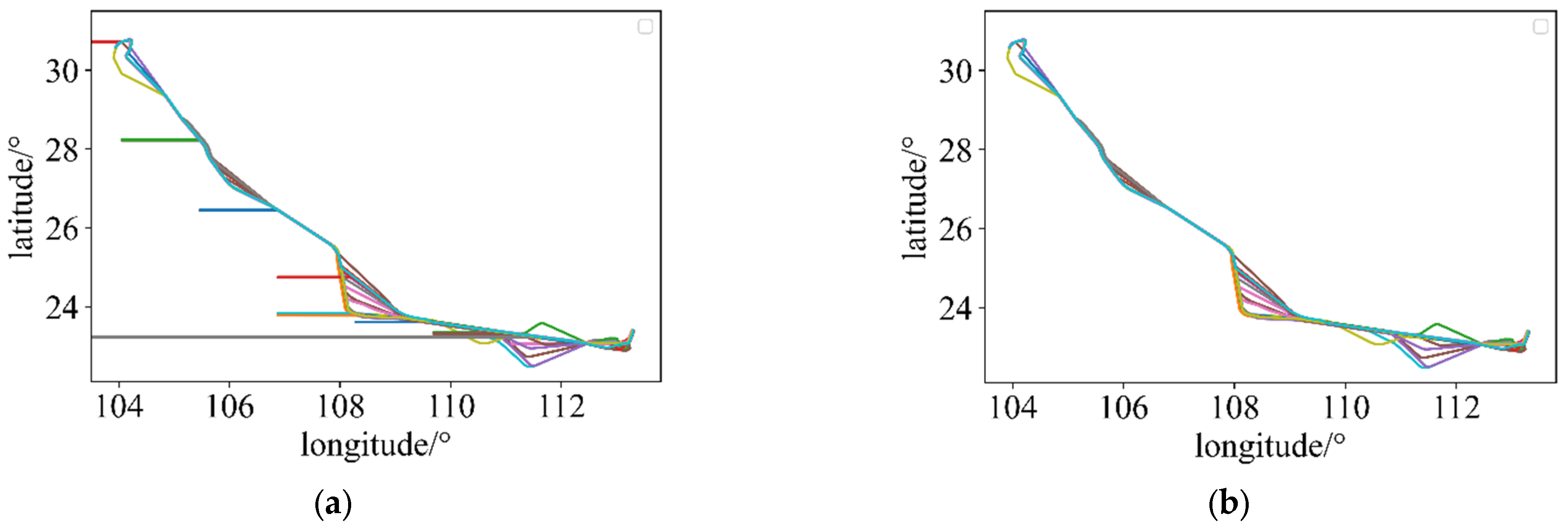
Due to the system error and other reasons, the real QAR trajectory data have some problems such as missing and abnormal trajectory points [31,32]. The abnormal trajectory points are eliminated according to the distance limit between two adjacent points, and the missing trajectory points are filled by linear interpolation. As shown in Figure 1, the cleaned trajectory is smoother and more continuous in terms of longitude and latitude, which effectively guarantees the production of subsequent data sets.
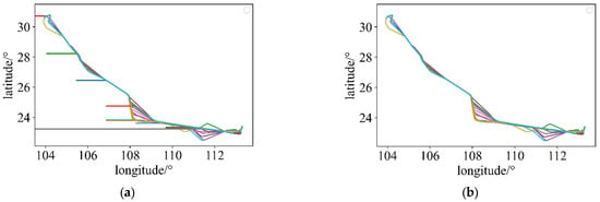
Figure 1.
Trajectory data cleaning, (a) before cleaning, (b) after cleaning.
2.3. Data Resampling
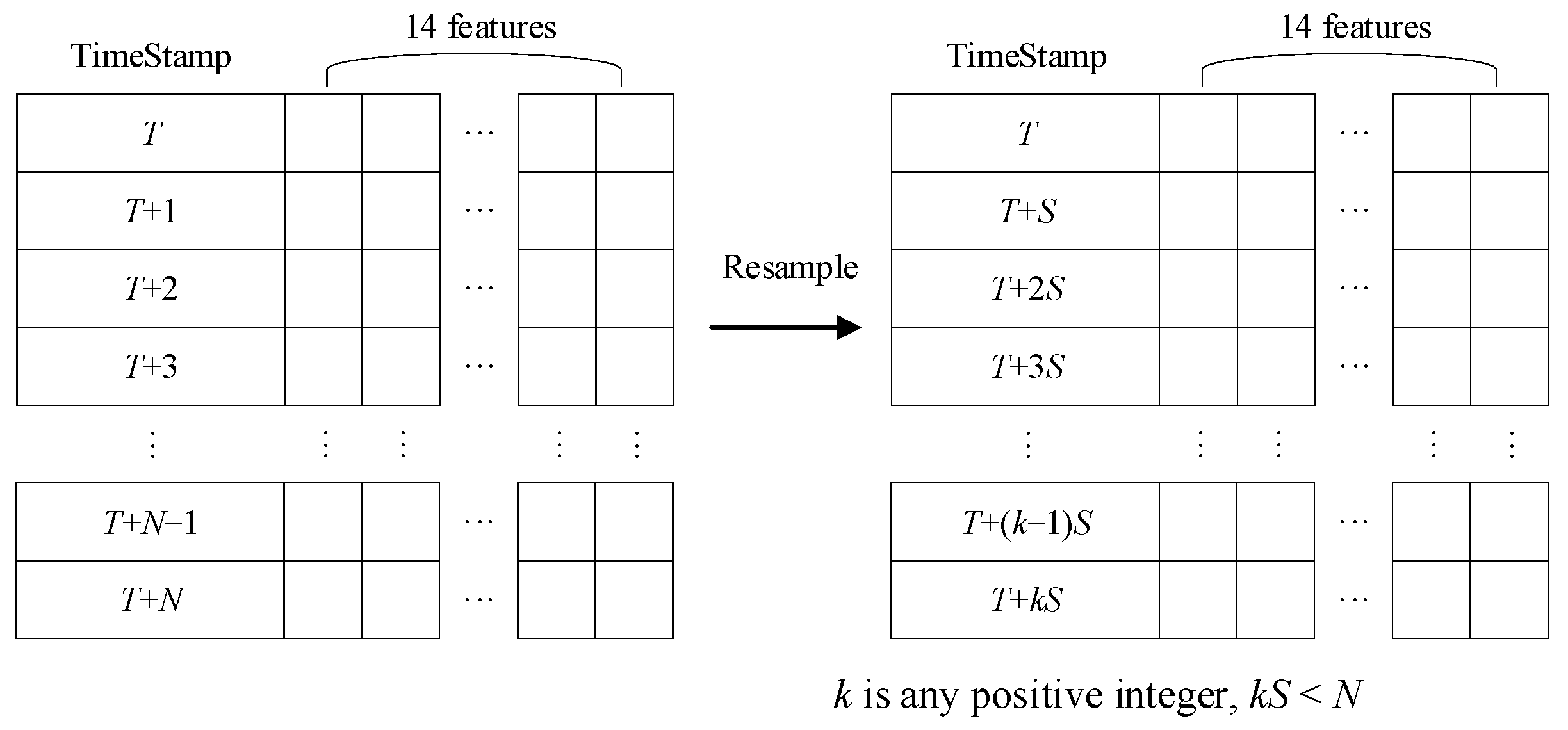
The traditional 4D trajectory prediction is to predict the next moment, longitude, latitude and altitude of the aircraft at the same time, and the prediction results have errors in four dimensions. Considering the perspective of time and assuming that the prediction of three-dimensional position coordinates is accurate enough, the overall deviation of trajectory points will also be caused by the error in time. Therefore, in order to avoid the error of time dimension, this paper converts the traditional 4D trajectory prediction to predict the 3D position of the aircraft at the next fixed moment. The features of class I are transformed into the timestamp. Assuming that the information recording time of a trajectory is between [T,T + N], the trajectory data are resampled with S as the sampling interval to obtain new trajectory data, as shown in Figure 2.
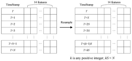
Figure 2.
Trajectory data resampling.
2.4. Data Normalization
The features of classes II, III and IV are processed as follows:
- (A).
- Min-max normalization
Min-max normalization, also known as deviation normalization [33], is a linear transformation of the original data that maps values between [0,1]. The conversion formula is as follows:
where max is the maximum value of the sample data, min is the minimum value of the sample data, and max–min is the range. For class II features, the above deviation standardization processing is adopted to retain the existing relationship in the original data, and effectively eliminate the influence of dimension and data value range.
- (B).
- Decimal scale normalization
The feature value is mapped between [–1,1] by moving the number of decimal places of the eigenvalue, depending on the maximum value of the absolute value of the eigenvalue [33]. The conversion formula is as follows:
For class Ⅲ features, the decimal scale normalization retains the positive and negative signs on the basis of eliminating the dimension and retains the characteristics of the original data to the greatest extent.
- (C).
- Feature encoding
For class IV features, the initial classification has been given for the original QAR data, which is processed by encoding (Table 2). Since the performance of the aircraft presents different characteristics in different flight phases, the numeralization of the flight phases preserves the progressive levels and differences between different phases while encoding them.

Table 2.
Flight phase feature coding.
2.5. Feature Transformation
The heading and wind direction in class Ⅴ features have obvious orientation, which has an important influence on the position change of the aircraft at the next moment. The action mode is closely related to the current operating state of the aircraft. However, the original numerical representation cannot fully express the influence on the aircraft operation, so it is necessary to transform heading and wind direction.
- (A).
- Heading
Based on original data, the value range of heading is [0,360]. If the value is transformed into [0,1] by the deviation standardization method, it is difficult to reflect the influence of heading on the change of longitude and latitude coordinates. Therefore, the feature transformation of heading is carried out, and the calculation formula is as follows:
where, HEAD is the heading; HEAD_LON is the sinusoidal heading; HEAD_LAT is the cosine heading.
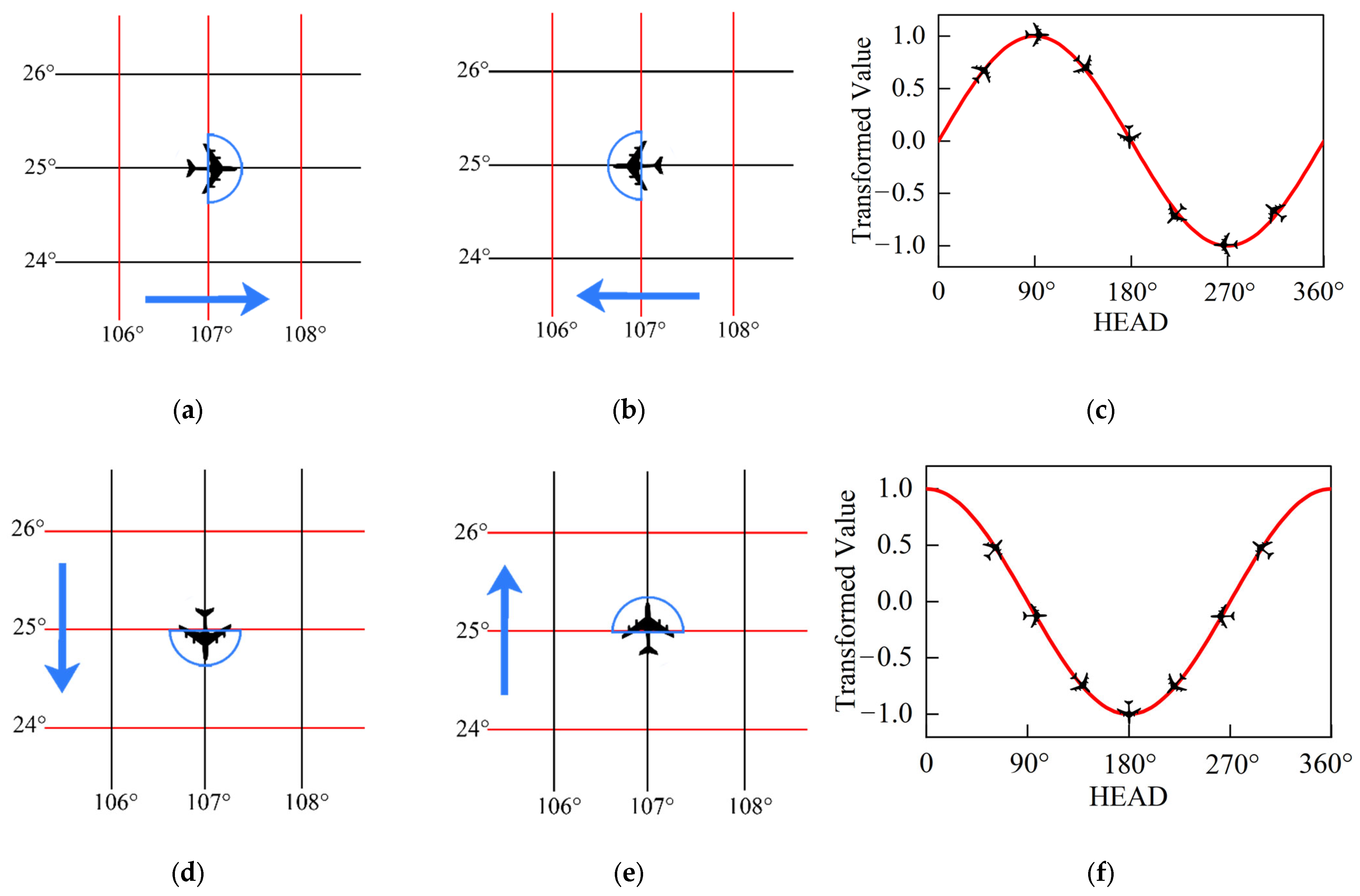
As for the longitude, when the heading is 90°, the direction of aircraft operation is perpendicular to the longitude and consistent with the direction of longitude increase (Figure 3a). As the heading increases to one hundred eighty degrees or decreases to zero degrees, the trend of longitude increase gradually decreases. When the heading is 270°, the direction of aircraft operation is perpendicular to the longitude and consistent with the direction of the decreasing longitude (Figure 3b). As the heading increases or decreases to 360° or 180°, the trend of decreasing longitude is more obvious. If positive and negative signs are used to represent the increasing and decreasing trends, and numerical values are used to represent the changing trend, the sine function can exactly represent the changing characteristics of longitude with heading (Figure 3c). Similarly, the cosine function can be used to represent the variation characteristics of latitude with heading (Figure 3d–f).
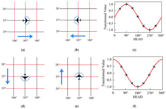
Figure 3.
Schematic diagram of heading change: (a) heading value [0,180]; (b) heading value [180,360]; (c) sinusoidal heading for longitude; (d) heading value [90,270]; (e) heading value [270,360] and [0,90]; and (f) cosine of heading for latitude.
- (B).
- Wind direction
Based on original data, the value range of the wind direction is [0,360], which is difficult to fully show the influence of the wind direction on the operation of the aircraft. Therefore, the feature transformation of the wind direction is carried out, and the calculation formula is as follows:
where, WD is the wind direction, WD′ is the transformed wind direction.
First, the absolute value of the difference between wind direction and heading is taken. When the absolute value exceeds 90°, the aircraft operates under the headwind condition, and the larger the angle, the more significant the effect of hindering aircraft operation (Figure 4a). When the absolute value is less than 90 °, the aircraft operates under downwind conditions, and the smaller the angle, the more significant the effect of promoting aircraft operation (Figure 4b). If positive and negative signs are used to represent downwind and headwind conditions, and numerical values are used to show the influence of trend, the cosine function can be used to accurately represent the changing characteristics of aircraft under the interaction between wind direction and heading (Figure 4c).

Figure 4.
Schematic diagram of wind direction change: (a) headwind; (b) downwind; (c) wind direction transform.
3. 4D Trajectory FDFP Model Based on the LSTM Network
3.1. LSTM Neural Network Theory
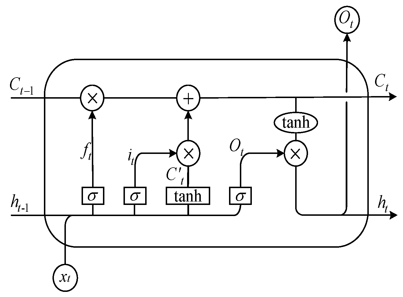
The LSTM neural network is one of the most representative time series data modeling methods in machine learning, consisting of an input layer, hidden layer and output layer. The hidden layer includes input gate, forget gate and output gate [34]. The structure is shown in Figure 5. The forget gate is the core of LSTM, through which information needs to be forgotten in order to realize the coexistence of short- and long-time information.

Figure 5.
Single LSTM cell structure.
The internal calculation method of LSTM is shown in the following formulas [34]:
where: ft is the probability that the information of the forgotten gate passes through; σ and tanh are Sigmoid functions and tanh functions; W is the weight matrix; h is the output of memory; x is the input of memory; b represents the bias matrix; it is the output of the input gate; Ct represents the state of memory; C’t is the candidate state; and Ot is for the output gate.
3.2. Selection of Influencing Factors
The flight phase, longitude, latitude, altitude, velocity, Mach number, wind speed and transformed wind direction at the presequence time are closely related to the position information at the prediction time, and the above features are called common features. Combined with the different characteristics of longitude, latitude and altitude, the feature matrix of the corresponding model is composed of the common feature group and their own unique features. The unique features of each dimension are shown in Table 3. Among them, the longitude model and latitude model select the sinusoidal heading and cosine heading respectively according to the action principle of heading in Section 2.5. The altitude model selects the pitch angle and pitch rate according to the altitude characteristics. The three models correspond to horizontal acceleration, lateral acceleration and vertical acceleration respectively according to the directionality of longitude, latitude and altitude. The above three models constitute the FDFP model. In the OP model of the comparison experiment, all the above features are considered as the feature matrix of the model for trajectory prediction.

Table 3.
Model influencing factor selection.
3.3. Model Training and Prediction
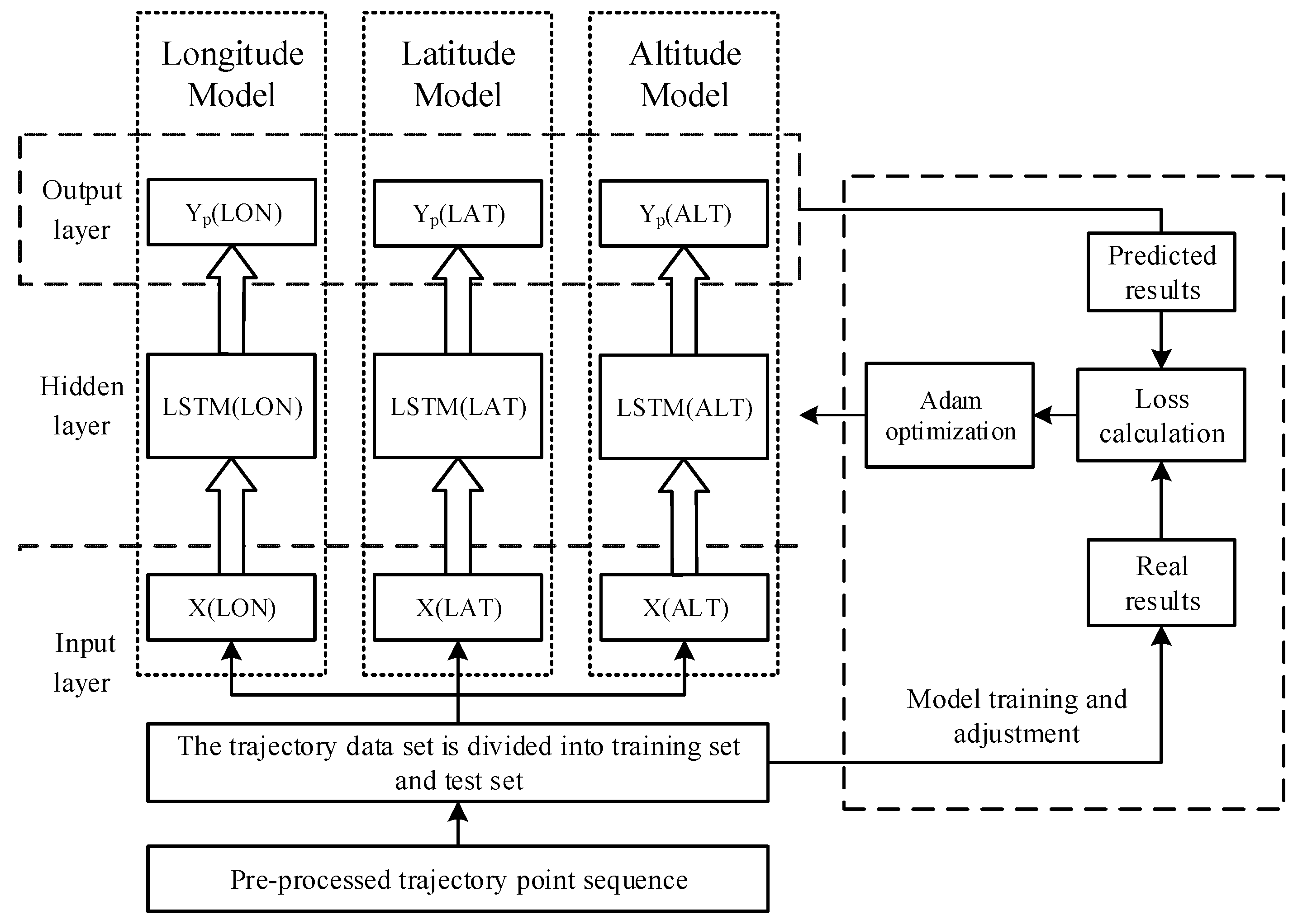
The 4D Trajectory FDFP model is based on the LSTM network. Firstly, data from trajectory point sequence are preprocessed and the training set and test set are divided. Then, according to three kinds of prediction targets, different feature matrices and labels are considered as sample data sets, which are input into the constructed longitude model, latitude model and altitude model for training and prediction. Finally, the model is optimized by calculating the loss between the predicted value and the actual value, and the final model is obtained. The specific process is shown in Figure 6. However, the OP model takes all the trajectory features as the feature matrix, and uses an LSTM network to predict longitude, latitude and altitude at the same time. In the process of aircraft operation, the trained model obtains QAR data in real time for trajectory prediction.
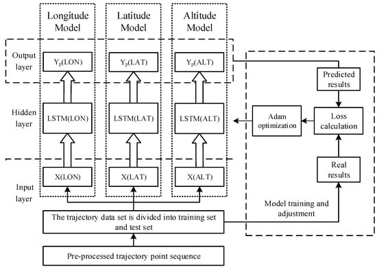
Figure 6.
FDFP model training flow chart.
3.4. Evaluation Indicators
Considering the error evaluation of regression problems and the sensitive detection of outliers, this paper uses the mean absolute error (MAE) and root mean square error (RMSE) to evaluate the effectiveness of prediction results. The calculation formulas are as follows:
where: Ypi is the ith predicted value, Yi is the ith true value, and n is the number of sample data.
In trajectory prediction, horizontal error and vertical error can be used to evaluate the accuracy of position prediction. The horizontal error is calculated by the Euclidean distance of two trajectory points, and the vertical error is the altitude difference between two trajectory points. In China’s actual air traffic control, the approach control should not be less than 6 km in the standard of radar horizontal interval, and the altitude layer should be separated by 300 m below 8400 m. Therefore, the horizontal error in the range of 3 km and the vertical error in the range of 150 m are selected. In this paper, the proportion of trajectory points in different error ranges will be used to evaluate the accuracy of the prediction model. The specific indicators and symbols are shown in Table 4.

Table 4.
Predictive indicators and symbols.
4. Experiment and Discussion
4.1. Data Set
The data used in this experiment are the real operation data of fixed urban routes from Chengdu Shuangliu Airport to Guangzhou Baiyun Airport from December 2021 to March 2022, totaling 671 trajectories. The data of 550 trajectories are taken as the training set for model training and verification, and the remaining 121 trajectories are used as the test set for prediction effect testing. Considering the input requirements of the LSTM model, a single trajectory sequence is used as the unit for data segmentation, and the historical trajectory data with a fixed step length is used to predict the position information of the next trajectory point.
4.2. Experimental Environment and Model Parameters
The experimental environment is Windows 10, a 64-bit operating system and NAVIDIA T600 graphics card. The LSTM model used is implemented on the Keras deep-learning platform based on Tensorflow. The optimal model structure and parameter setting are obtained through continuous experiments by the trial-and-error method. (Table 5). There are some constraints on the parameter setting. For example, in order to fully learn the few cases in the data set such as INIT. CLIMB and FINAL phase, the batch size will be set smaller and the training time will be considered, which will naturally set the epoch smaller.

Table 5.
Model parameters.
4.3. Comparative Analysis of Experimental Results
The trained model is used to predict 121 untrained trajectories in the test set one by one. The prediction results are plotted, and the relevant evaluation indexes are calculated.
4.3.1. Single Trajectory Prediction
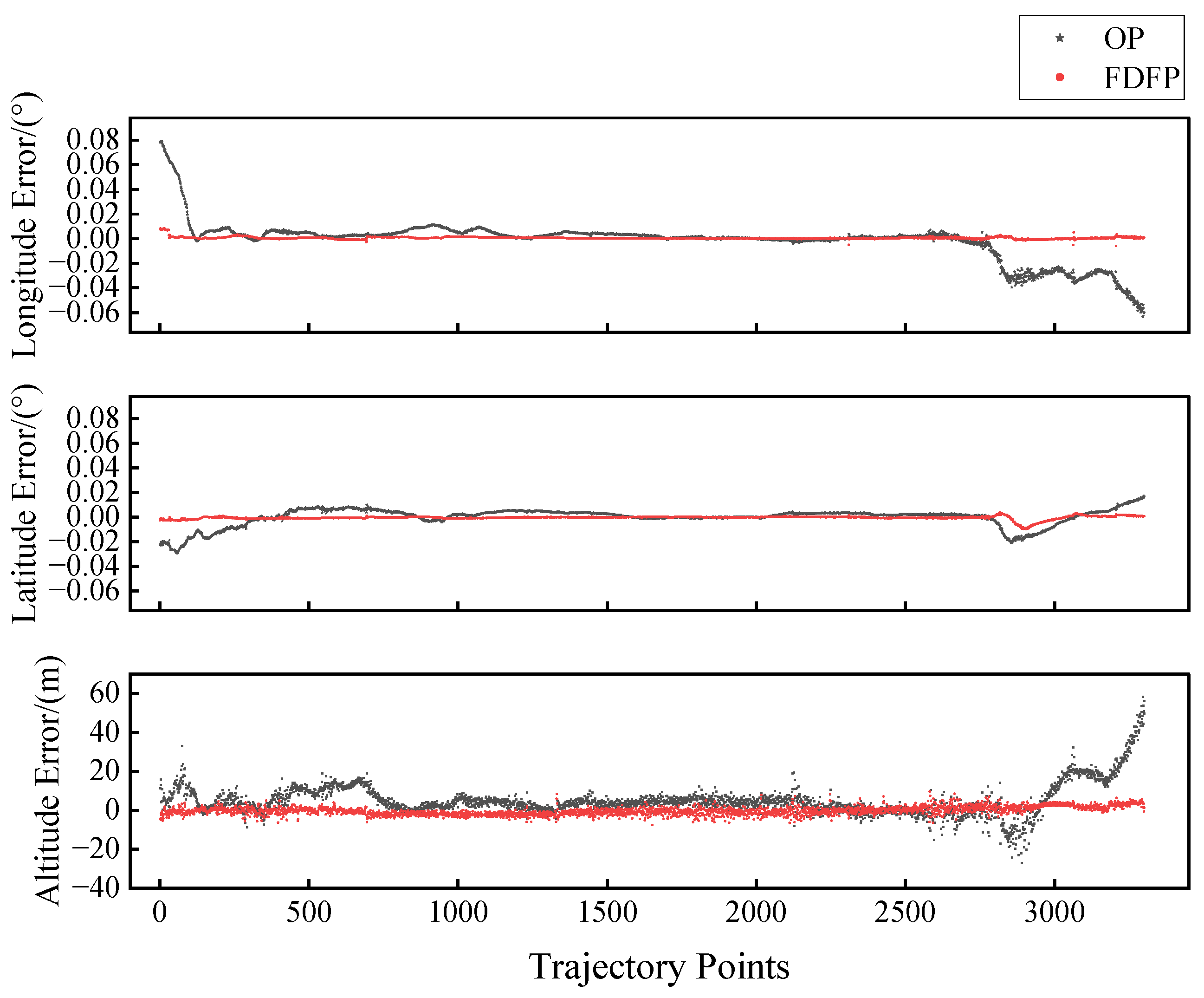
Taking a certain trajectory as an example, the OP model and the FDFP model proposed in this paper are respectively used for trajectory prediction, and the errors of each dimension are shown in Figure 7.
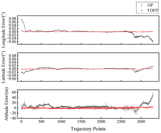
Figure 7.
Errors in each dimension of single trajectory prediction.
Since aircraft are greatly affected by air traffic control during climbing and descending, and trajectory fluctuations are frequent, the prediction result of the two models is more preferable in the cruise phase. The errors of the OP model in the three dimensions have obvious fluctuations, especially in the climbing and descending, and the fluctuation range is large. Considering the same order of magnitude, the prediction error of longitude is significantly larger than that of latitude. The imbalance of multi-dimensional prediction accuracy is also a common problem in the OP model. In comparison, the FDFP model has better performance, with smaller prediction errors and less fluctuation, and performs more accurate prediction when the aircraft is climbing and descending.
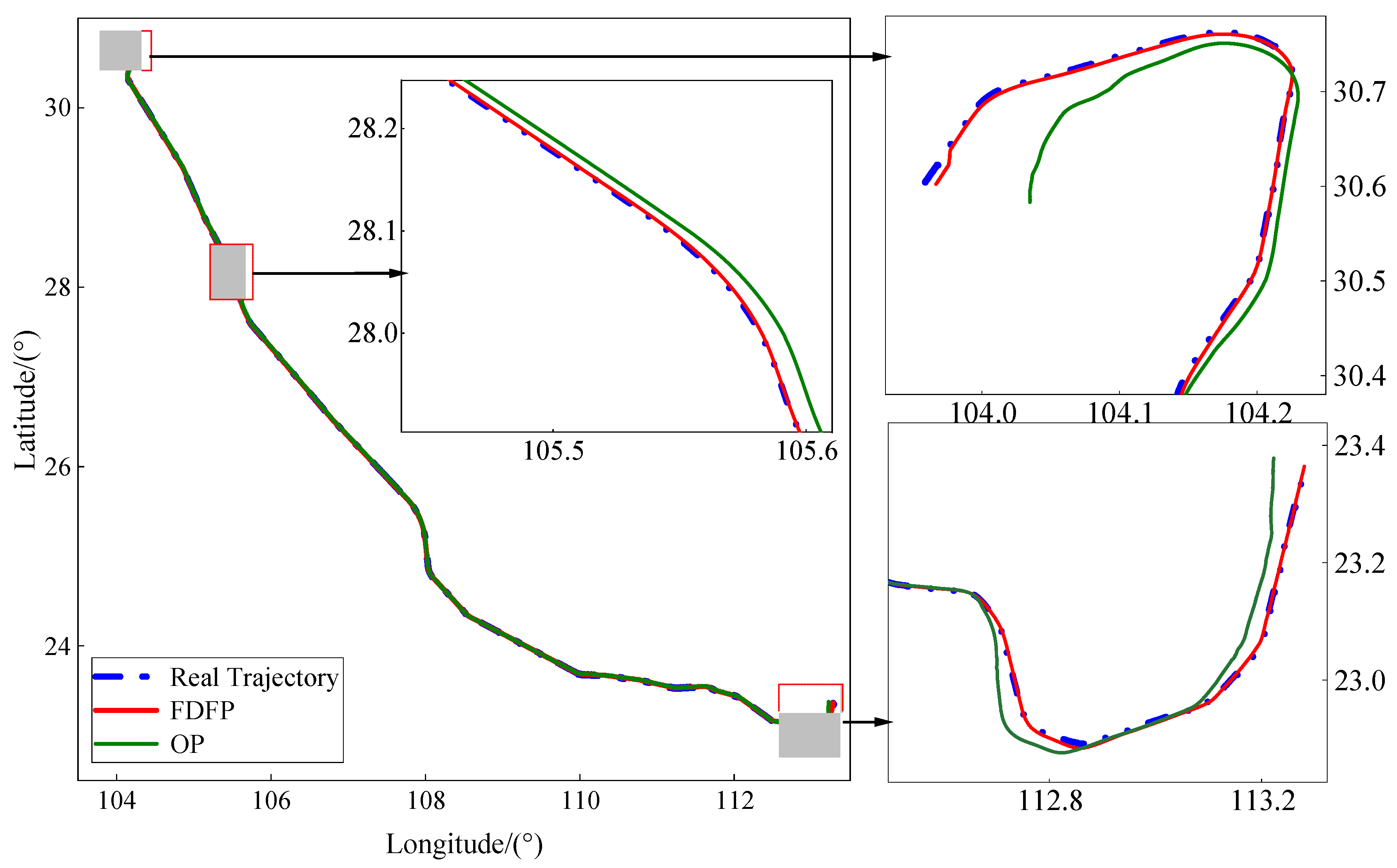
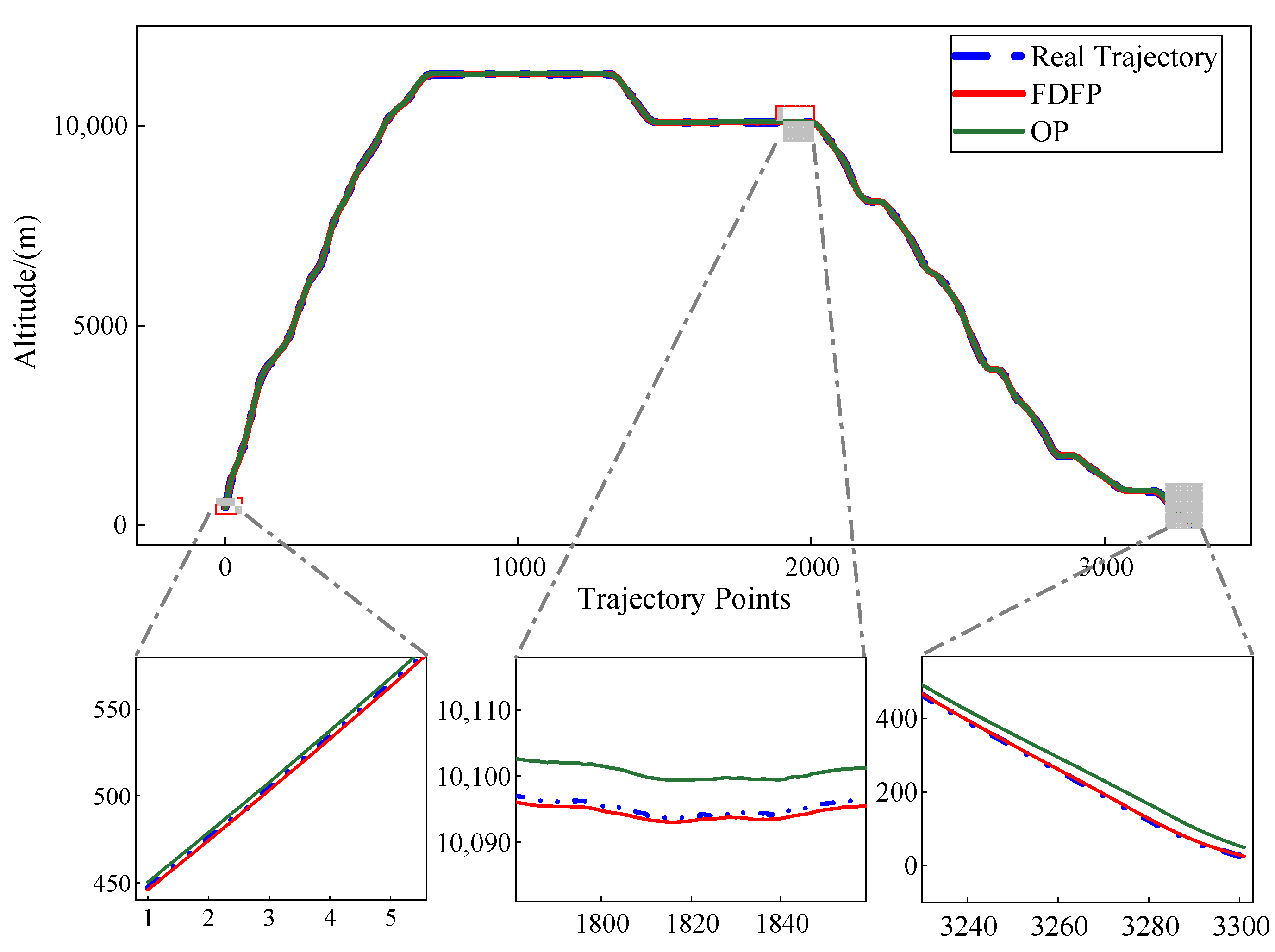
The comparison between the real trajectory and the predicted trajectory is shown in Figure 8 and Figure 9. In Figure 8, both models can accurately predict the overall operation trend of the aircraft. From the partially enlarged drawing of the cruise phase, the overall predicted trajectory is significantly different from the real trajectory, while the fractal dimension feature (FDF)-predicted trajectory can better match the real trajectory. This is because the OP model has learned the trend of trajectory change, but it is not sensitive to specific values. During the climbing and descending phases of the aircraft, the overall predicted trajectory is not smooth, and there is a large deviation from the real trajectory. The closer to the end of the trajectory, the more significant the deviation degree. However, the FDF predicted trajectory has excellent performance, and the trajectory curve is smooth and stable, which could be well consistent with the real trajectory. There is only a small deviation at the head of the trajectory, and the deviation degree is much smaller than that of the overall predicted trajectory. The reason is that the running time is short at this phase, and there are fewer samples for model learning and training.
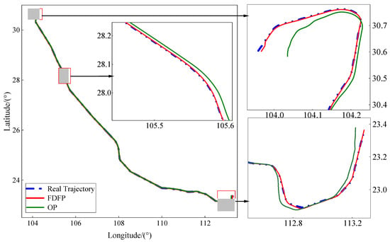
Figure 8.
Longitude and latitude variation diagram of single trajectory.
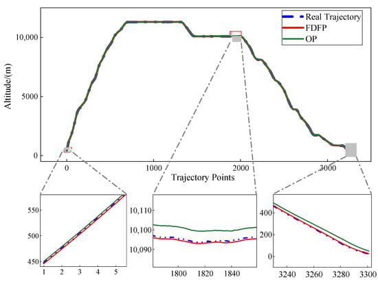
Figure 9.
Altitude variation chart for single trajectory.
As can be seen from Figure 9, the two models are accurate in predicting the trend of altitude change. According to the local enlarged images A, B and C, which compare the prediction results of the three phases with the actual trajectory, the prediction results of the FDFP model are more stable and accurate than those of the OP model.
The evaluation indexes of each prediction result are shown in Table 6 and Table 7 and Figure 10. It can be seen that the evaluation indexes of the FDFP model are better than the OP model, and the MAE of three dimensions are reduced by 92%, 84% and 74% on average, showing a good performance in horizontal error. It takes about 30 ms to predict the position of a trajectory point by using the FDFP model, which is far less than the sampling interval of 2 s, which meets the conditions of real-time prediction.

Table 6.
Comparison of MAE and RMSE for single trajectory prediction.

Table 7.
Comparison of horizontal error and vertical error for single trajectory prediction.
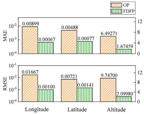
Figure 10.
Comparison of MAE and RMSE for single trajectory prediction.
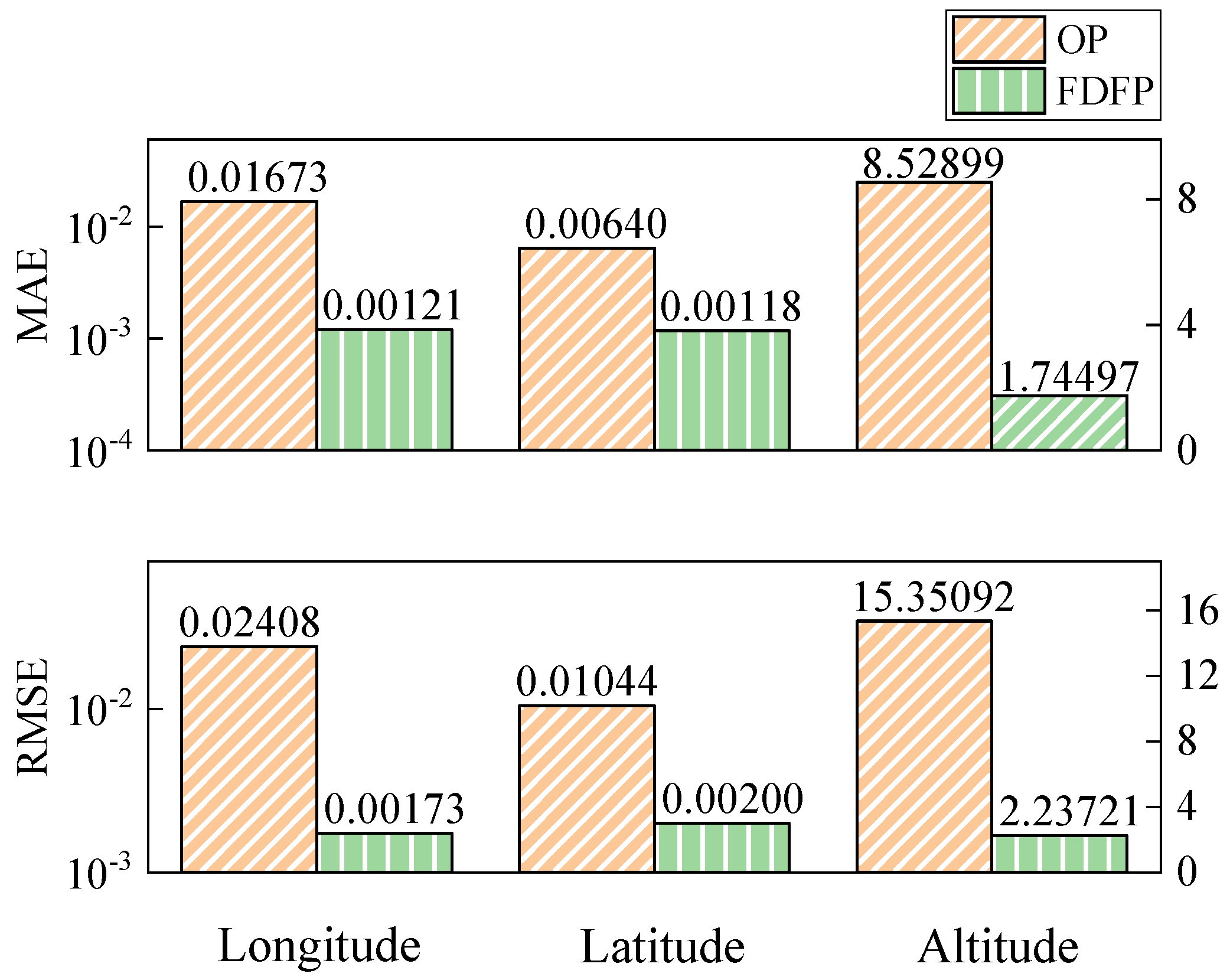
4.3.2. Multiple Trajectory Prediction
The prediction results of 121 trajectories in the test set are compared with the actual results, as shown in Table 8 and Table 9 and Figure 11. In the FDFP model, the MAE of predicted longitude and latitude are both less than 0.0015°, the MAE of altitude is less than 2 m, and the horizontal error within the range of 3 km, 1 km and 500 m accounts for 100%, 97.77% and 91.71%, respectively. Compared with the OP results, the MAE of the three dimensions is reduced by 92%, 81% and 79%, respectively, and the prediction accuracy is significantly improved. Compared with the prediction accuracy of the longitude and latitude of the same dimensional features, in the OP model, the longitude MAE reaches 2.6 times that of the latitude MAE, while the FDFP is less than 1.1 times. It can be seen that the FDFP model is more stable and more accurate in predicting the spatial position of trajectory points.

Table 8.
Comparison of MAE and RMSE for multi-trajectory prediction.

Table 9.
Comparison of horizontal error and vertical error for multi-trajectory prediction.
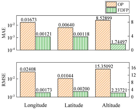
Figure 11.
Comparison of MAE and RMSE for multi-trajectory prediction.
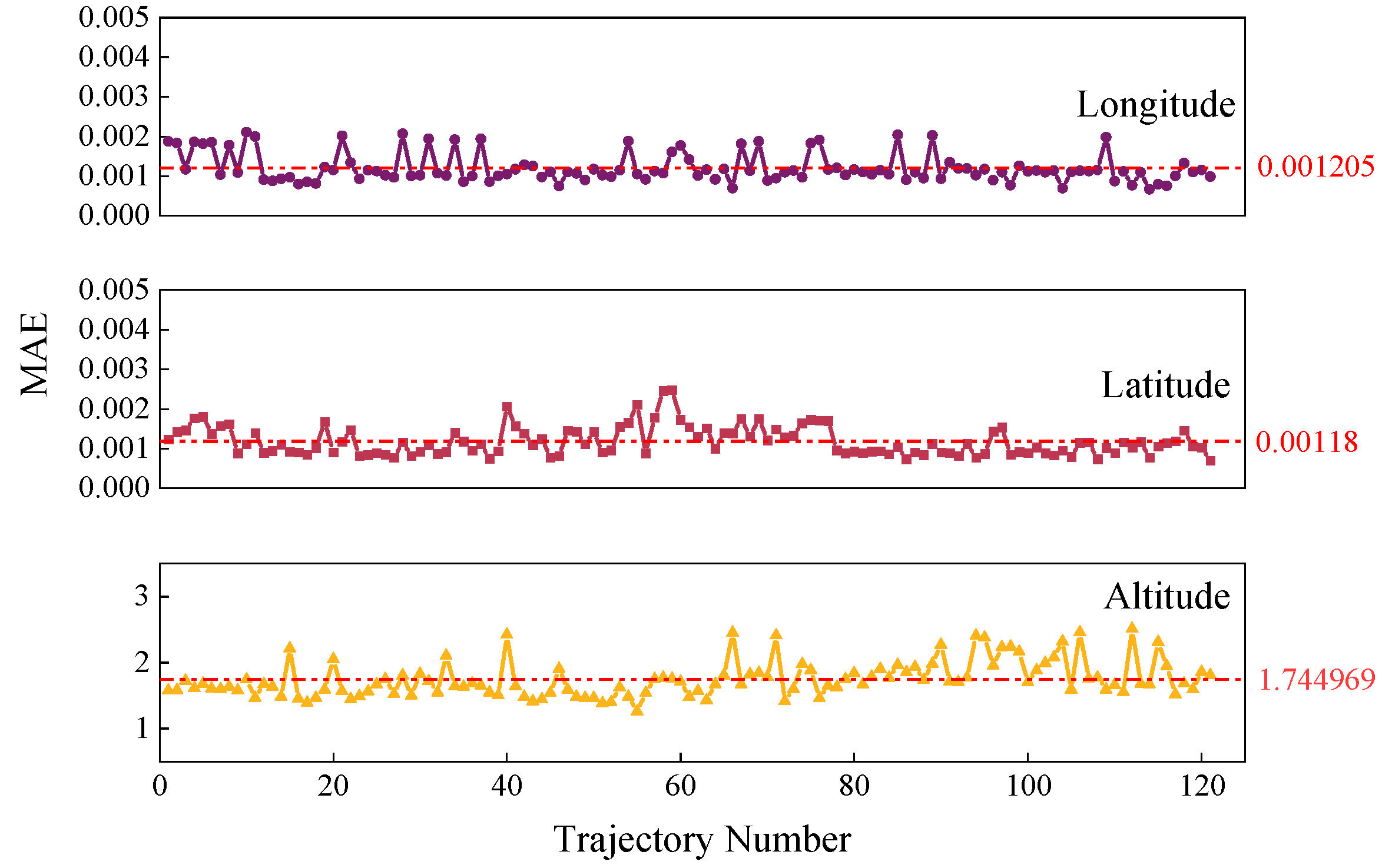
The MAE values of 121 trajectory prediction results are shown in Figure 12, where the dashed lines are the average MAE values of each dimension. Compared with each trajectory, the prediction accuracy of the three dimensions is stable and converges to a certain range, which shows the good robustness of the FDFP model.

Figure 12.
MAE value for multi-trajectory prediction.
4.3.3. Assessment of the Impact of Feature Transformation on Trajectory Prediction
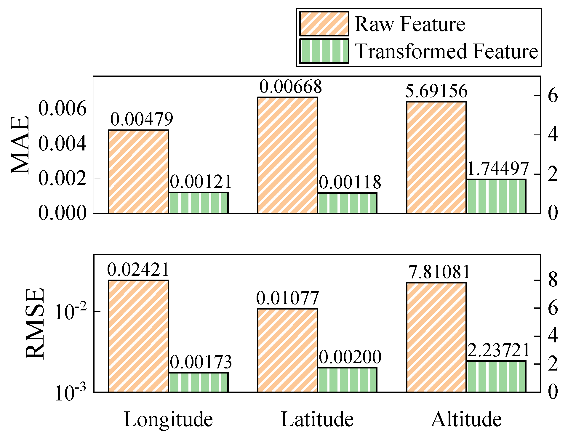
In order to verify the influence of heading and wind direction feature transformation on trajectory prediction in Section 2.5, the sample data sets of raw features and transformed features are respectively adopted, and the FDFP model is used to predict the trajectory of the test set. The results are shown in Table 10 and Table 11, and Figure 13. Compared with the prediction results of raw features, the MAE of transformed features in the three dimensions is reduced by 75%, 82% and 69% respectively; the horizontal error is also greatly reduced. The results show that the feature transformation of heading and wind direction can effectively improve the accuracy of trajectory prediction.

Table 10.
Comparison of MAE and RMSE for feature transformation.

Table 11.
Comparison of horizontal error and vertical error for feature transformation.
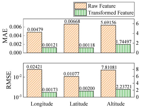
Figure 13.
Comparison of MAE and RMSE for feature transformation.
4.3.4. Trajectory Prediction under Special Conditions
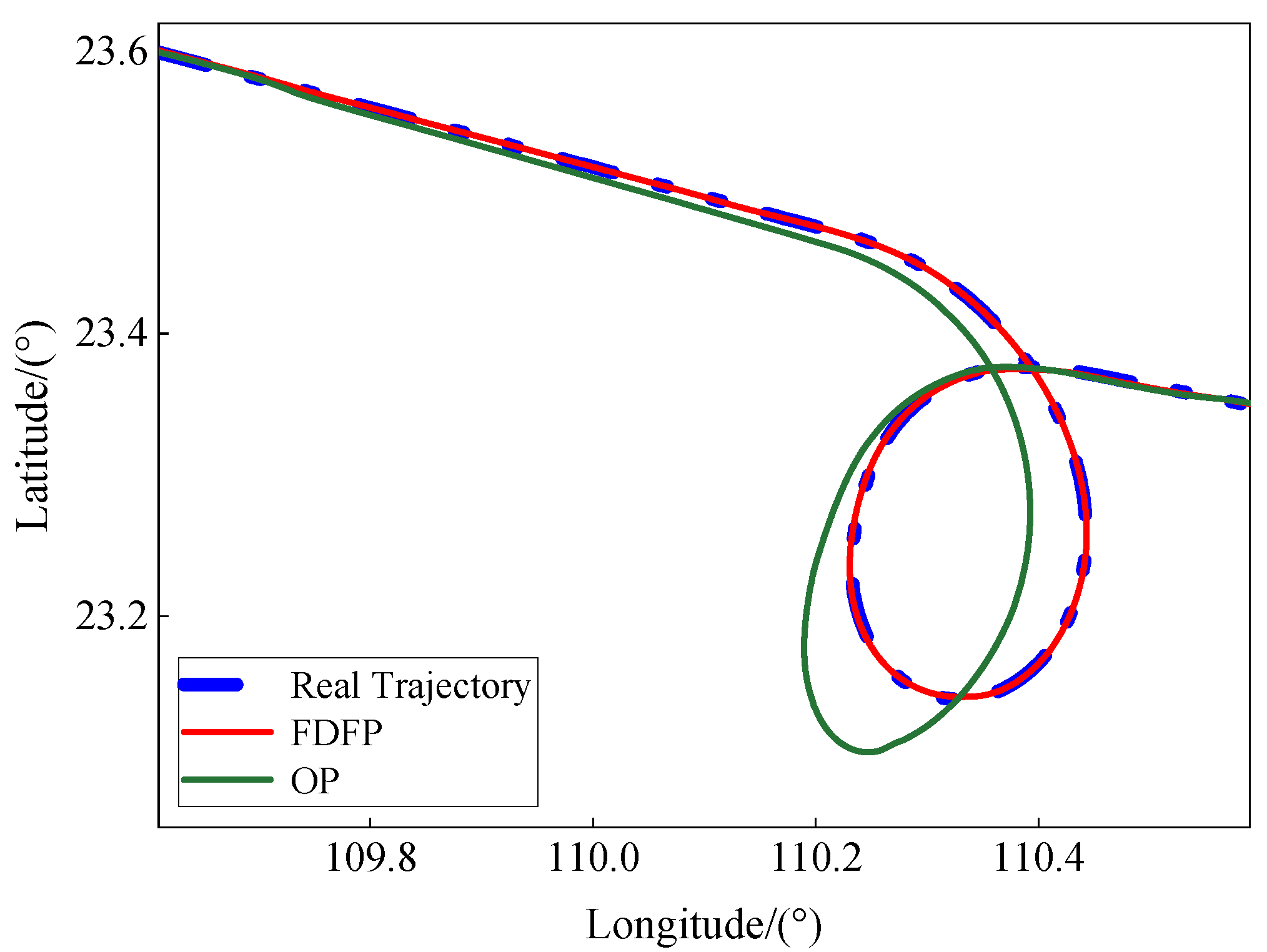
Under the influence of bad weather, flow management, airport capacity limitation and so on, special conditions such as circling could appear in aircraft operation. In order to investigate the prediction result of the model in this paper under special conditions, a trajectory with circling phase is selected from the test set and its prediction results are analyzed. The changes in longitude and latitude in the circling phase are shown in Figure 14. Before circling, the predicted trajectory of the OP and FDFP models are in good agreement with the real trajectory. As the circling continues, the predicted trajectory of the OP model starts to deviate from the real trajectory, and there is a significant deviation in the circling phase during the big turn, while the predicted trajectory of the FDFP model always overlaps with the real trajectory. At the end of the circling, the three trajectories converge again.
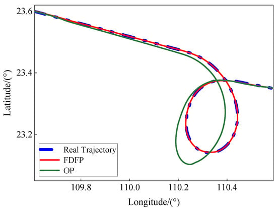
Figure 14.
Trajectory prediction in circling phase.
The prediction results for this trajectory in the circling phase are shown in Table 12. The MAE of the OP model is bigger, showing that the OP model cannot make an accurate prediction of the special phase, and that the FDFP model is better than the OP model in three dimensions, demonstrating that the FDFP model for the special phase can also have accurate prediction results.

Table 12.
MAE of the two forecasting models in the circling phase.
4.3.5. Trajectory Prediction at Multi-Sampling Interval
In order to improve the long-term performance of the real-time prediction, trajectory data test sets with sampling intervals of 2 s, 6 s and 10 s are used for comparative experiments. The evaluation indicators are shown in Table 13. The prediction errors for longitude, latitude and altitude will increase with the widening in sampling interval. Taking the 10 s sampling interval with the largest error as an example, the MAE of longitude and latitude are less than 0.008°, and the MAE of altitude is less than 9 m. Meanwhile, the prediction errors of the three dimensions are more balanced, which reflects the good robustness of the model.

Table 13.
Comparison of MAE and RMSE at different sampling intervals.
4.3.6. Robustness Verification of FDFP Model
In order to verify the robustness of the FDFP model, the LSTM network is replaced by gradient boosting (XGBoost) to conduct the comparison experiment between the FDFP model and OP model. The results displayed in Table 14 show that the prediction effect of the FDFP model is better than that of the OP model in all dimensions, which reflects the robustness of the FDFP model.

Table 14.
Comparison of prediction results of two forecasting models based on XGBoost.
4.4. Discussion
In this paper, the FDFP model based on QAR data is proposed to improve the accuracy of trajectory prediction. In order to verify the validity and robustness of the FDFP model, single trajectory prediction, multi-trajectory prediction, trajectory prediction under special conditions, under multi-sampling interval and under different basic models are respectively used to compare the FDFP model with the OP model, which is widely used in previous studies. The results show that FDFP model can achieve better prediction performance through each evaluation indicators.
First, in terms of longitude and latitude prediction, the predicted trajectory of FDFP model is almost consistent with the real trajectory (Figure 7 and Figure 8), and also has a good performance under special conditions (Figure 14), indicating that the FDFP model based on LSTM can learn the rule of trajectory change. However, it is inevitable that the prediction error at both ends of the trajectory is large. The introduction of the PDFP model can alleviate this problem to a certain extent. Second, in the aspect of altitude prediction (Figure 7 and Figure 9), FDFP model stabilizes the prediction effect and narrows down the error range compared with the OP model. In the end, the paper also conducts comparative experiments on the proposed feature transformation (Table 10 and Table 11 and Figure 13), which further improves the prediction accuracy.
5. Conclusions
In this paper, the FDFP model is constructed using the QAR historical trajectory data based upon the combination of different influencing factors. The QAR data can be acquired in real time for trajectory prediction, which shows an excellent prediction result in the experiment. At the same time, the feature transformation of heading and wind direction also significantly improves the prediction accuracy of the model. Based on the LSTM network and XGBoost, this paper verifies the effectiveness of the FDFP model, which makes full use of QAR data features to improve both the accuracy and real-time response of trajectory prediction. It promotes the implementation of the TBO and the sustainable development of air traffic management.
However, this study also has some limitations. First of all, although there are still technical barriers to the availability of QAR data, its rich trajectory characteristics can bring different effects to the problem of trajectory prediction compared with ADS-B and radar data. Therefore, it is very necessary to conduct prospective research on QAR data. Secondly, the FDFP model will increase the number of models and occupy more memory. However, in order to improve the prediction accuracy, this sacrifice is considered worthwhile. Future research can consider model compression to save memory. Finally, the historical data used in the experiment only has a fixed urban route, and its application scope is limited. More data can be collected to solve the problem of data limitation in subsequent studies.
In the future, the abundant trajectory features brought by QAR data should be paid full attention to, and the availability of QAR data should be improved from a technical standpoint. In order to improve the accuracy of trajectory prediction, it is necessary to conduct targeted data preprocessing and flexibly transform the original trajectory features. At the same time, the selection of models can be more diversified, not limited to the LSTM network and XGBoost, and suitable models can be selected according to the characteristics of different prediction dimensions, prediction accuracy and other requirements.
Author Contributions
Conceptualization, Y.Z. and K.L.; Methodology, Y.Z. and K.L.; Software, K.L.; Validation, K.L.; Writing-original draft preparation, K.L.; writing-review and editing, Y.Z.; Visualization, K.L. All authors have read and agreed to the published version of the manuscript.
Funding
National Natural Science Foundation of China (62173332); Tianjin Science and Technology Planning Project (21JCYBJC00700); Open Fund for Key Laboratory of Civil Aviation Flight Wide-area Surveillance and Safety Control Technology (202106).
Data Availability Statement
The data presented in this study are available on request from the corresponding author.
Conflicts of Interest
The authors declare no conflict of interest.
References
- Hao, S.; Cheng, S.; Zhang, Y. A multi-aircraft conflict detection and resolution method for 4-dimensional trajectory-based operation. Chin. J. Aeronaut. 2018, 31, 1579–1593. [Google Scholar] [CrossRef]
- Joint Planning and Development Office. Concept of Operations for the Next Generation Air Transportation System; Joint Planning and Development Office: Washington, DC, USA, 2007. [Google Scholar]
- Undertaking, S.J. The European ATM Master Plan, Edition 2, October 2012. Available online: https://www.atmmasterplan.eu/download/25 (accessed on 30 October 2012).
- Baştanlar, Y.; Özuysal, M. Introduction to machine learning. Mirnomics MicroRNA Biol. Comput. Anal. 2014, 1107, 105–128. [Google Scholar]
- De, L.A.; Paassen, M.; Mulder, M. A machine learning approach to trajectory prediction. In Proceeding of the AIAA Guidance, Navigation, and Control (GNC) Conference, Boston, MA, USA,, 23 August 2013. [Google Scholar]
- Tastambekov, K.; Puechmorel, S.; Delahaye, D.; Rabut, C. Aircraft trajectory forecasting using local functional regression in Sobolev space. Transp. Res. Part C Emerg. Technol. 2014, 39, 1–22. [Google Scholar] [CrossRef]
- Kanneganti, S.T.; Chilson, P.B.; Huck, R. Visualization and Prediction of Aircraft trajectory using ADS-B. In Proceeding of the NAECON 2018-IEEE National Aerospace and Electronics Conference, Dayton, OH, USA, 23–26 July 2018. [Google Scholar]
- Wang, T.; Huang, B. Fuzzy Cluster Analysis of 4D Trajectory Based on ADS-B. J. Traffic Inf. Saf. 2013, 31, 38–42. [Google Scholar]
- Georgiou, H.; Pelekis, N.; Sideridis, S. Semantic-aware aircraft trajectory prediction using flight plans. Int. J. Data Sci. Anal. 2020, 9, 215–228. [Google Scholar] [CrossRef]
- Wang, Z.; Liang, M.; Delahaye, D. Short-term 4d trajectory prediction using machine learning methods. In Proceeding of the SID, Fuzhou, China, 18–20 February 2017. [Google Scholar]
- Barratt, S.T.; Kochenderfer, M.J.; Boyd, S.P. Learning probabilistic trajectory models of aircraft in terminal airspace from position data. IEEE Trans. Intell. Transp. Syst. 2018, 20, 3536–3545. [Google Scholar] [CrossRef]
- Wu, X.; Yang, H.; Chen, H. Long-term 4D trajectory prediction using generative adversarial networks. Transp. Res. Part C Emerg. Technol. 2022, 136, 103554. [Google Scholar] [CrossRef]
- Pang, Y.; Yao, H.; Hu, J. A recurrent neural network approach for aircraft trajectory prediction with weather features from sherlock. In Proceeding of the AIAA Aviation 2019 Forum, Dallas, TX, USA, 17–21 June 2019. [Google Scholar]
- Alligier, R.; Gianazza, D.; Durand, N. Machine learning and mass estimation methods for ground-based aircraft climb prediction. IEEE Trans. Intell. Transp. Syst. 2015, 16, 3138–3149. [Google Scholar] [CrossRef]
- Li, X.; Pi, J.; Huang, F. Self-generated deep neural network based 4D trajectory prediction. J. Comput. Appl. 2021, 41, 1492. [Google Scholar]
- Pang, Y.; Liu, Y. Conditional generative adversarial networks (CGAN) for aircraft trajectory prediction considering weather effects. In Proceeding of the AIAA Scitech 2020 Forum, Orlando, FL, USA, 6–10 January 2020. [Google Scholar]
- Yang, K.; Bi, M.; Liu, Y. LSTM-based deep learning model for civil aircraft position and attitude prediction approach. In Proceeding of the 2019 Chinese Control Conference (CCC), Guangzhou, China, 27–30 July 2019. [Google Scholar]
- Shi, Z.; Xu, M.; Pan, Q. 4D Flight Trajectory Prediction with Constrained LSTM Network. IEEE Trans. Intell. Transp. Syst. 2020, 99, 1–14. [Google Scholar]
- Zhang, Z.; Yang, R.; Fang, Y. LSTM network based on on antlion optimization and its application in flight trajectory prediction. In Proceeding of the 2018 2nd IEEE Advanced Information Management, Communicates, Electronic and Automation Control Conference (IMCEC), Xi’an, China, 25–27 May 2018. [Google Scholar]
- Zeng, W.; Quan, Z.; Zhao, Z. A deep learning approach for aircraft trajectory prediction in terminal airspace. IEEE Access 2020, 8, 151250–151266. [Google Scholar] [CrossRef]
- Yue, J. Research on Short-term Trajectory Prediction Method and Visualization System Development Based on LSTM-ARIMA. Master’s Thesis, Civil Aviation University of China, Tianjin, China, 2020. [Google Scholar]
- Ma, L.; Tian, S. A Hybrid CNN-LSTM Model for Aircraft 4D Trajectory Prediction. IEEE Access 2020, 8, 134668–134680. [Google Scholar] [CrossRef]
- Pang, Y.; Xu, N.; Liu, Y. Aircraft Trajectory Prediction using LSTM Neural Network with Embedded Convolutional Layer. In Proceedings of the Annual Conference of the PHM Society, Scottsdale, AZ, USA, 23 September 2019. [Google Scholar]
- Zhang, P.; Yang, T. Feature Extraction and Prediction of QAR Data based on CNN-LSTM. Appl. Res. Comput. 2019, 36, 2958–2961. [Google Scholar]
- Liu, L.; Cui, L.; Han, Y. Aircraft trajectory prediction based on convLSTM. Comput. Eng. Des. 2022, 43, 1127–1133. [Google Scholar]
- Cui, Y.; Xiong, W.; He, Y. Adaptive forecast model for uncertain track. Acta Aeronaut. Et Astronaut. Sin. 2019, 40, 322557. [Google Scholar]
- Han, P.; Wang, W.; Shi, Q. Real-time Short-term Trajectory Prediction Based on GRU Neural Network. In Proceeding of the 2019 IEEE/AIAA 38th Digital Avionics Systems Conference (DASC), San Antonio, TX, USA, 8–12 September 2019. [Google Scholar]
- Shi, Q.; Wang, W. Short-term 4D Trajectory Prediction Algorithm Based on Online Updated LSTM Network. J. Signal Process. 2021, 37, 66–74. [Google Scholar]
- Wang, T.; Huang, B. A Four-dimensional Flight Trajectory Prediction Model based on Improved Kalman Filter. J. Comput. Appl. 2014, 34, 1812–1815. [Google Scholar]
- Zhang, J.; Liu, J.; Hu, R. Online four dimensional trajectory prediction method based on aircraft intent updating. Aerosp. Sci. Technol. 2018, 77, 774–787. [Google Scholar] [CrossRef]
- Cao, C.; Yu, H.; Liu, Y. Automatic Tracking Method of Basketball Flight Trajectory Based on Data Fusion and Sparse Representation Model. Complexity 2021, 2021, 9568753. [Google Scholar] [CrossRef]
- Chen, X.; Wu, S.; Shi, C. Sensing data supported traffic flow prediction via denoising schemes and ANN: A comparison. IEEE Sens. J. 2020, 20, 14317–14328. [Google Scholar] [CrossRef]
- Liu, M.J.; Wang, X.F.; Huang, Y.L. Data preprocessing in data mining. Comput. Sci. 2000, 27, 4. [Google Scholar]
- Zhou, S.; Guo, S.; Du, B. A Hybrid Framework for Multivariate Time Series Forecasting of Daily Urban Water Demand Using Attention-Based Convolutional Neural Network and Long Short-Term Memory Network. Sustainability 2022, 14, 1108. [Google Scholar] [CrossRef]
Disclaimer/Publisher’s Note: The statements, opinions and data contained in all publications are solely those of the individual author(s) and contributor(s) and not of MDPI and/or the editor(s). MDPI and/or the editor(s) disclaim responsibility for any injury to people or property resulting from any ideas, methods, instructions or products referred to in the content. |
© 2023 by the authors. Licensee MDPI, Basel, Switzerland. This article is an open access article distributed under the terms and conditions of the Creative Commons Attribution (CC BY) license (https://creativecommons.org/licenses/by/4.0/).

