
Study on Temperature Distribution Law of Tunnel Portal Section in Cold Region Considering Fluid–Structure Interaction

Abstract
:1. Introduction
2. The Basic Theory of Heat Conduction and Heat Convection Calculation in Cold Tunnel
2.1. Control Equation of Heat Conduction in Tunnel in Cold Region
2.2. Control Equation of Air Thermal Convection in Tunnel in Cold Region
- (1)
- Continuity equation
- (2)
- The Navier–Stokes (N-S) equations of motion
- (3)
- Energy-conservation equation
- ①
- Boundary conditions on the fluid–structure interface
- ②
- Heat balance condition of solid wall temperature
- ③
- Adiabatic solid wall conditions
- ④
- Kinematic, kinetic, and thermodynamic conditions at the fluid interface
3. Three-Dimensional Finite-Element Solution of Air Thermal Convection Model of Tunnel in Cold Region
3.1. Characteristic Line Operator-Splitting Finite-Element Method for N-S Equation
3.1.1. Operator Splitting of N-S Equation
3.1.2. The Display Time Discretization and Display Format of the Convection Term along the Characteristic Line
- (1)
- The display time discretization of the convection term along the characteristic line
- (2)
- Multi-step display format of convection term
3.1.3. Three-Dimensional Finite-Element Solution
- (1)
- Three-dimensional finite-element discretization of diffusion term
- (2)
- Three-dimensional finite-element discretization of convection term
- (3)
- Three-dimensional finite-element discretization of pressure Poisson equation
- (4)
- Three-dimensional finite-element discretization of velocity correction term
3.2. Explicit Characteristic Line–Galerkin Method for Energy-Conservation Equation
3.2.1. Explicit Characteristic Line–Galerkin Method
3.2.2. Three-Dimensional Finite-Element Solution
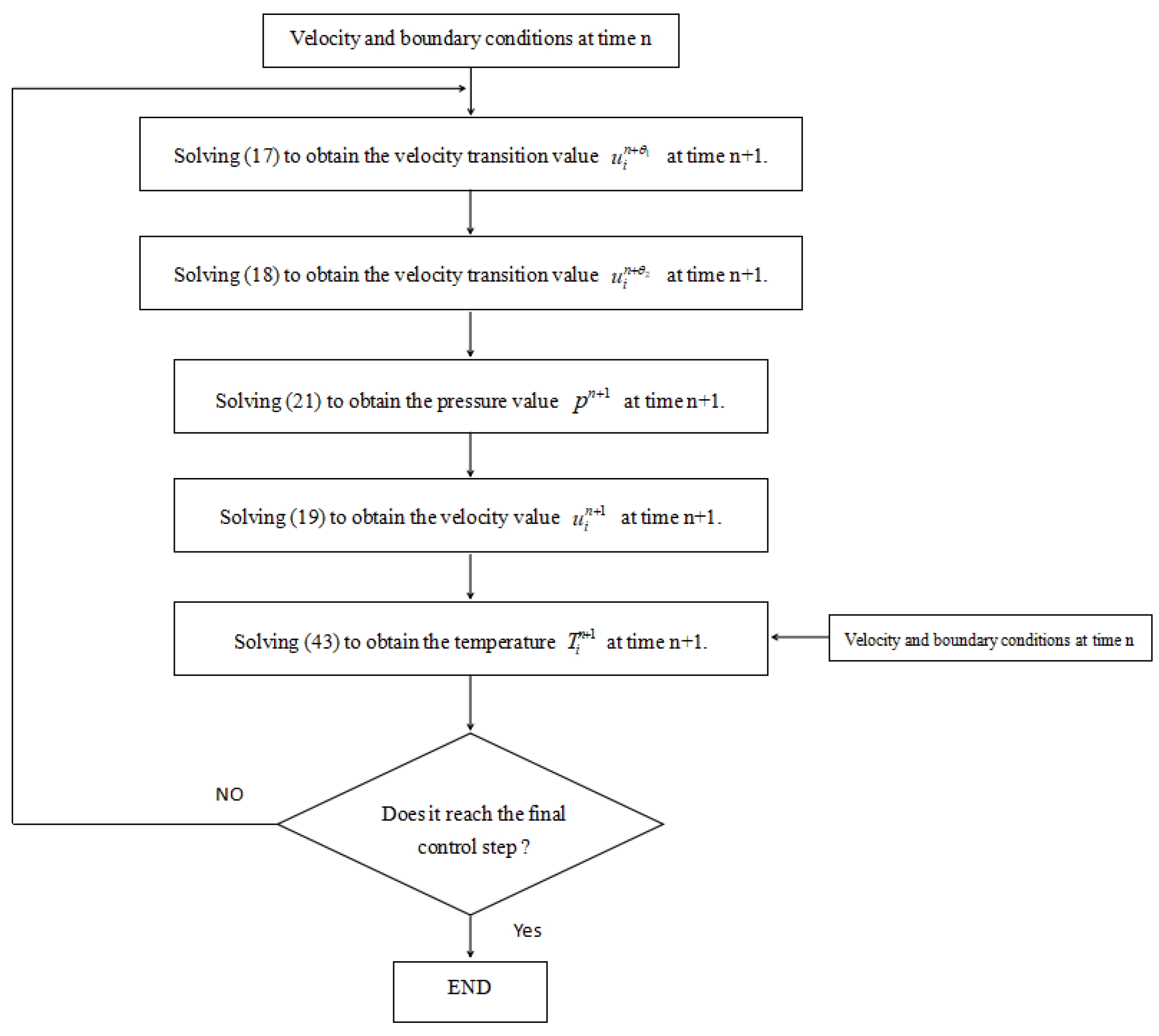
3.3. Algorithm Procedure
4. Numerical Solution of Heat Conduction-Heat Convection Fluid-Structure Interaction Model of Tunnel in Cold Region
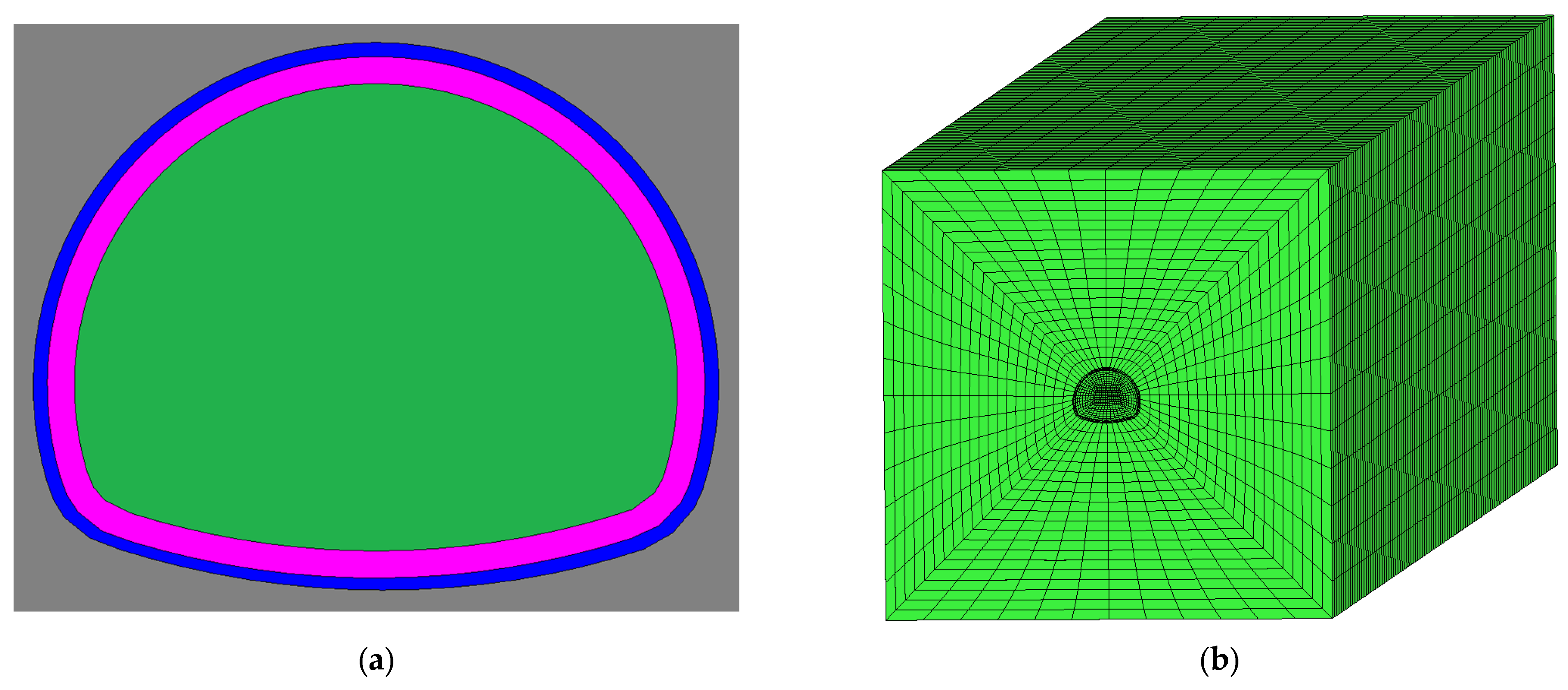
4.1. Model Introduction
- (1)
- Tunnel surrounding rock and lining heat transfer
- (2)
- Thermal convection of air in tunnel
- (3)
- Heat transfer between tunnel air and lining
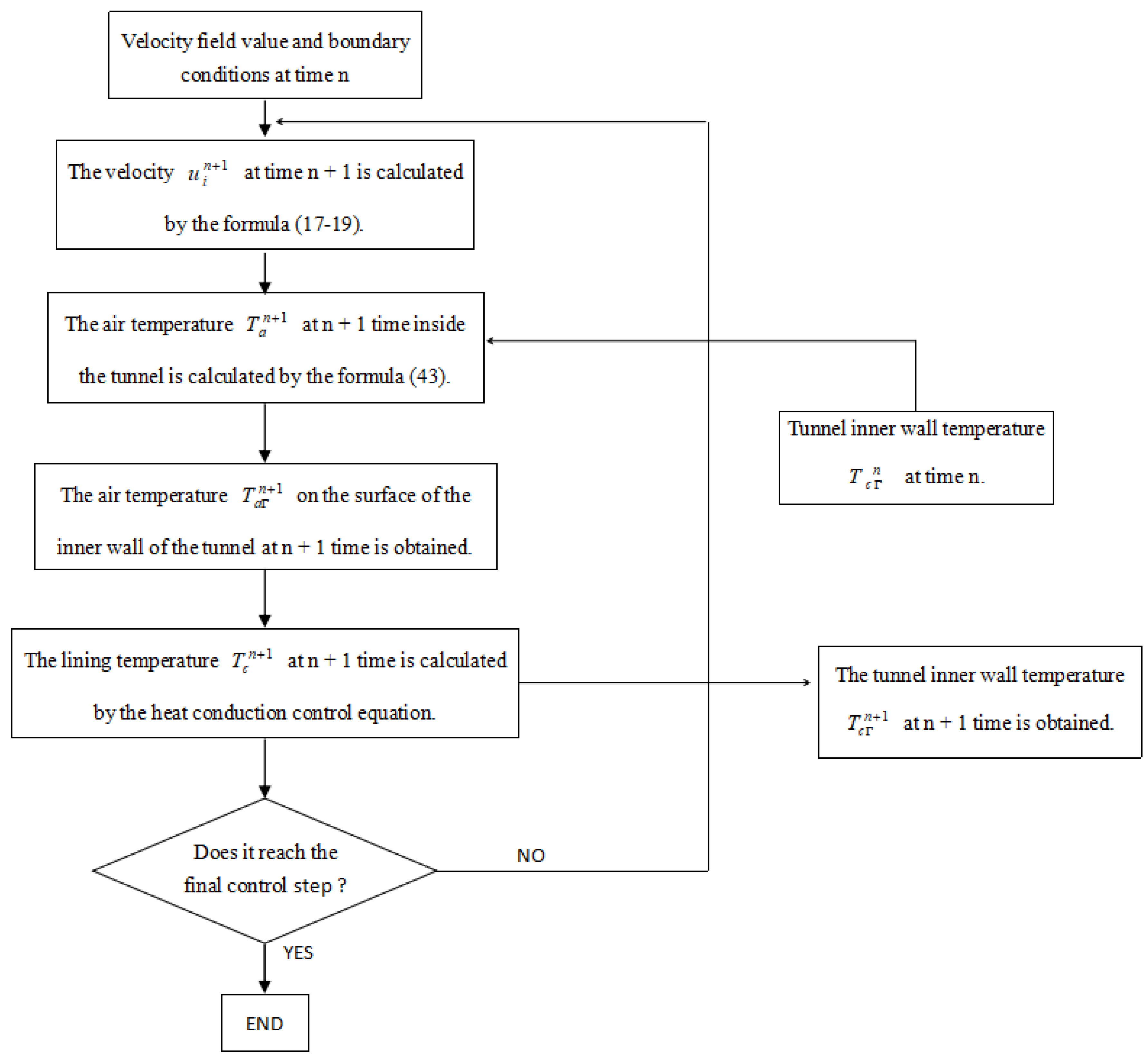
4.2. Algorithm Procedure
5. Application Example
5.1. Project Profile
5.2. Monitoring Scheme and Result Analysis
- (1)
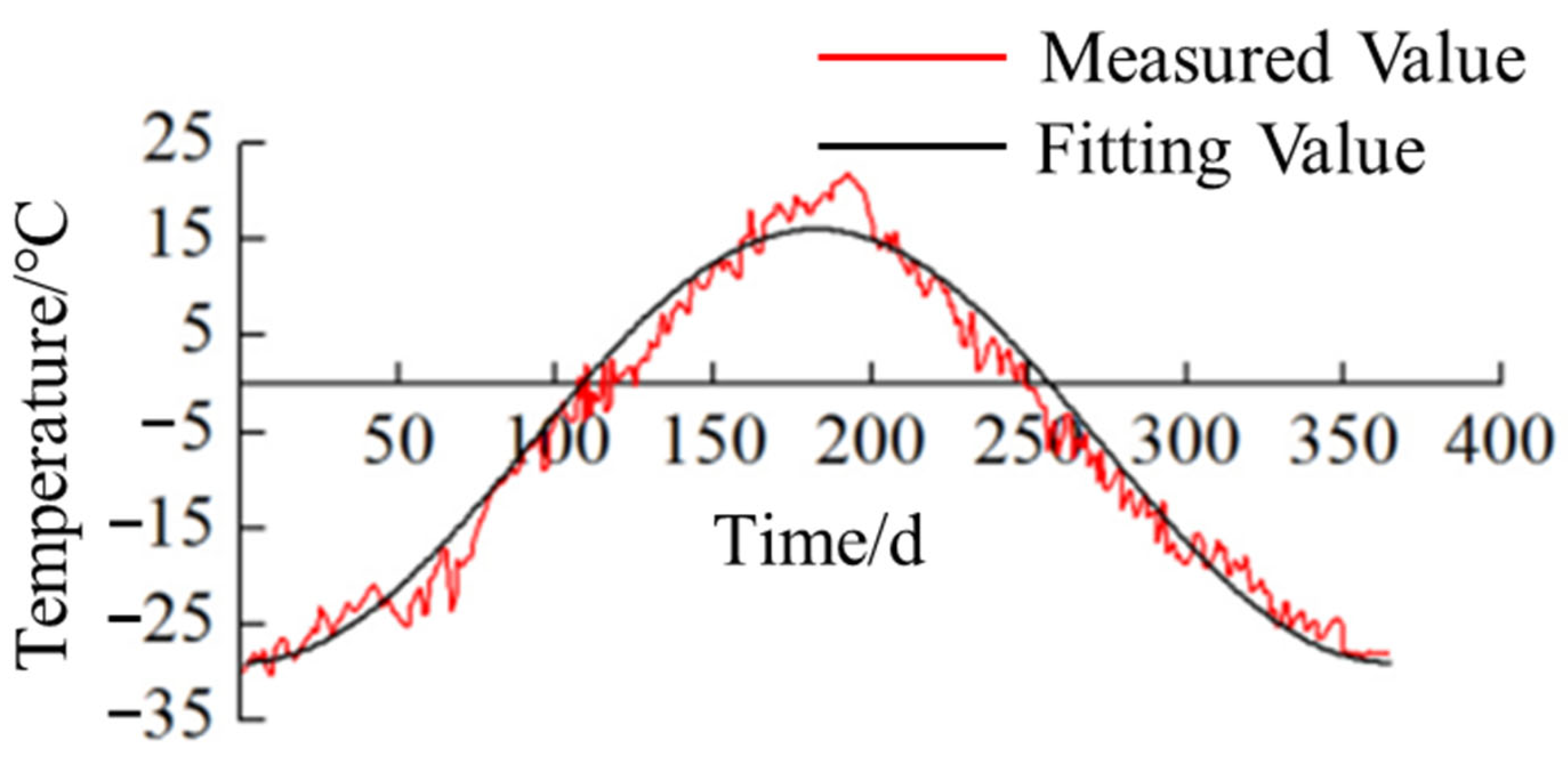
- Temperature change
- (2)
- Wind speed variation
- (3)
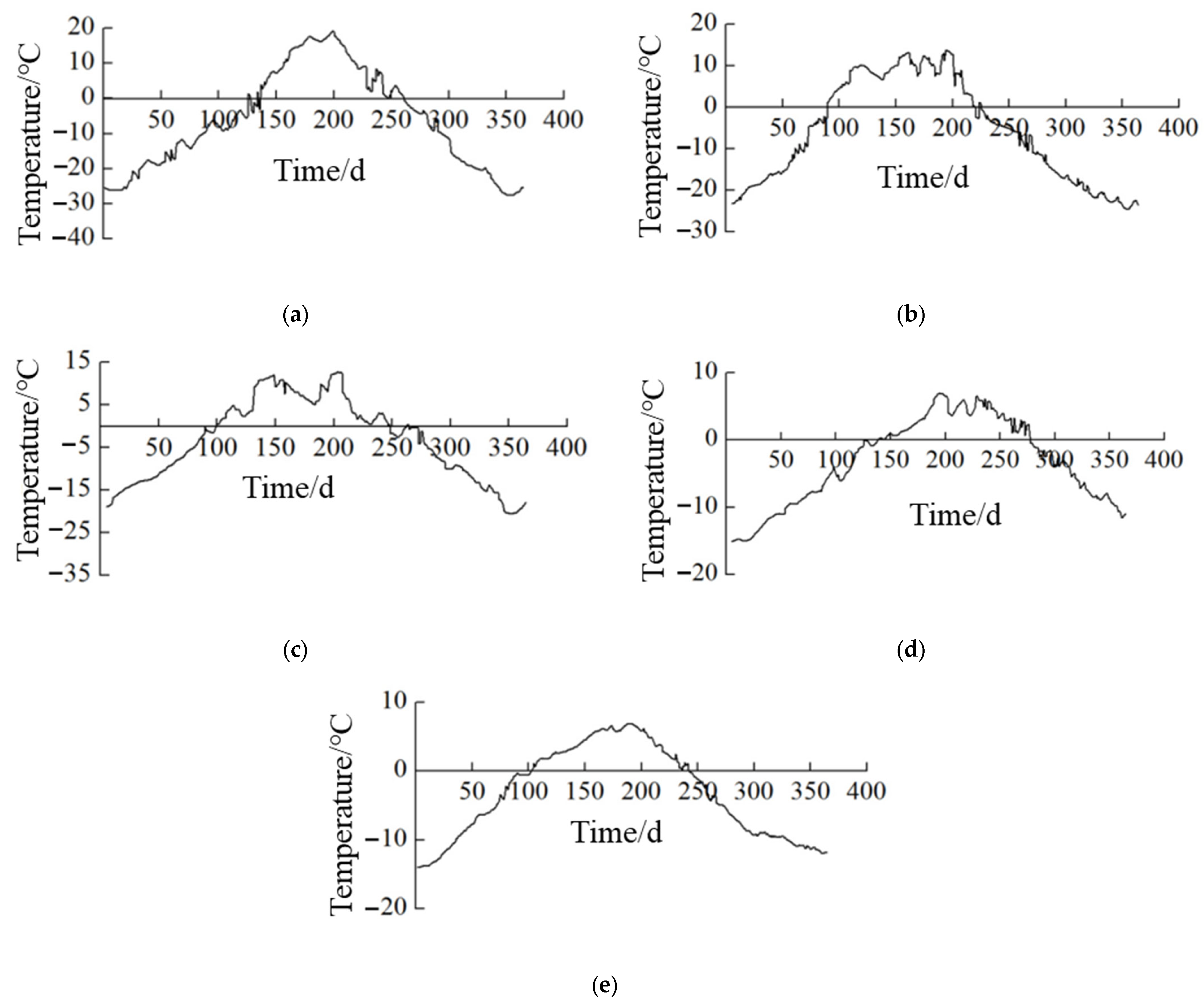
- Lining wall temperature change
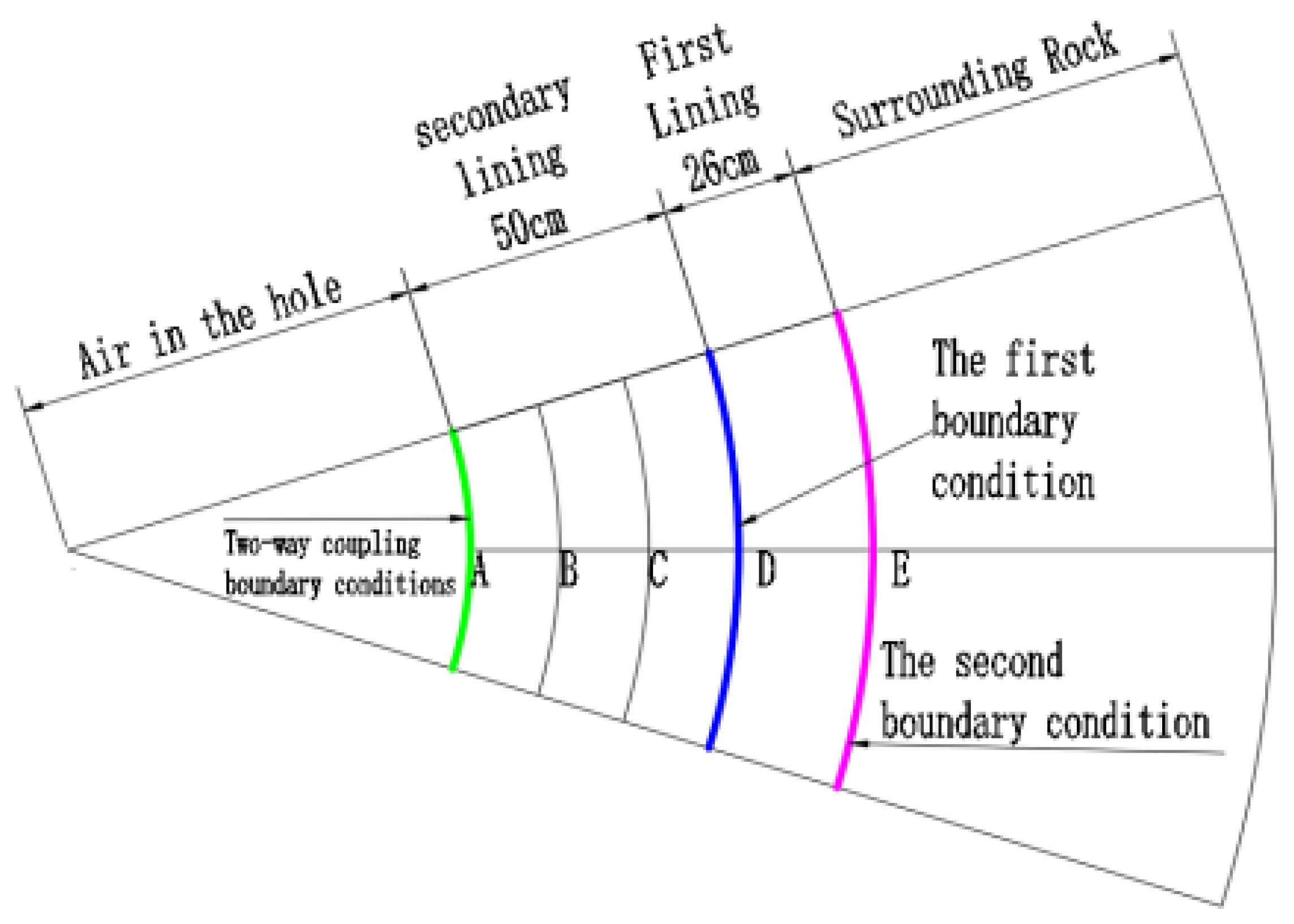
5.3. Calculation Model
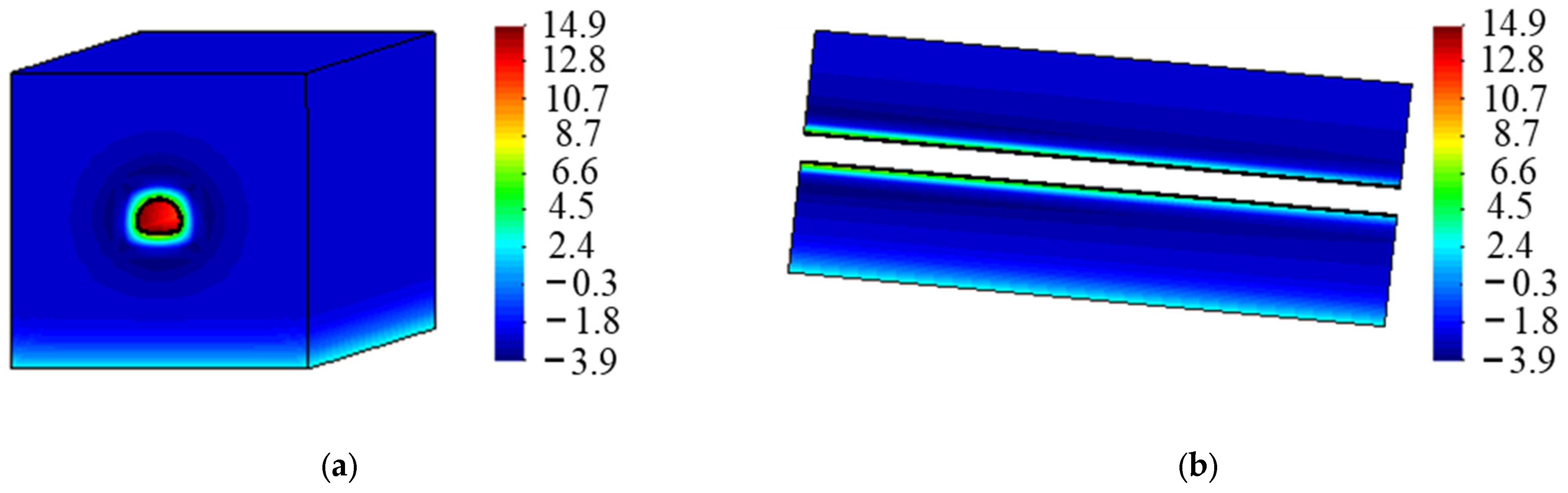
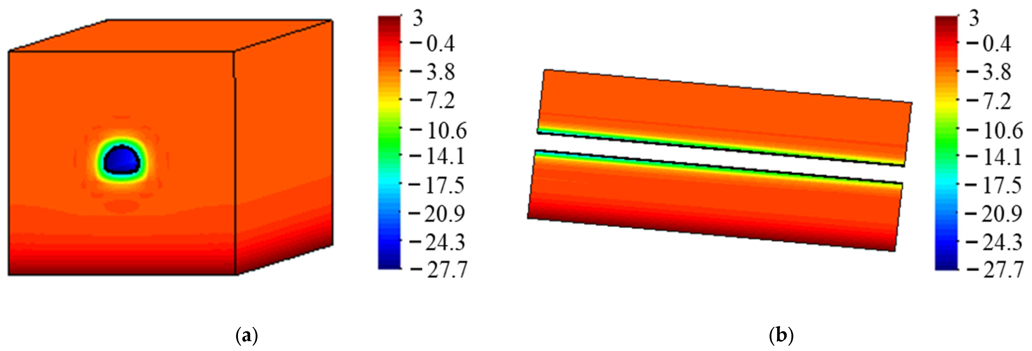
5.4. Verification and Analysis of Calculation Results
6. Conclusions
- (1)
- In terms of the idea of the characteristic-based operator-splitting (CBOS) finite-element method and the explicit characteristic–Galerkin method, a finite-element method for solving three-dimensional N-S equations and thermal convection governing equations is developed., and the velocity and temperature are coupled. A three-dimensional finite-element calculation model of air thermal convection in tunnels in cold regions is established. After the velocity and pressure are decoupled in the model, the same order interpolation function can be used, which greatly improves the calculation efficiency. Consequently, the calculation results can be of high accuracy.
- (2)
- Considering the dynamic influence of air velocity and temperature on the lining surface in the tunnel, the fluid–structure interaction finite-element calculation model of tunnels in cold regions is established by coupling the heat transfer model of the tunnel lining and surrounding rock with the air heat convection model. Compared with other calculation models, this model can fit the actual situation and more accurately reflect the distribution law of the lining temperature field and air temperature field in each layer of the tunnel.
- (3)
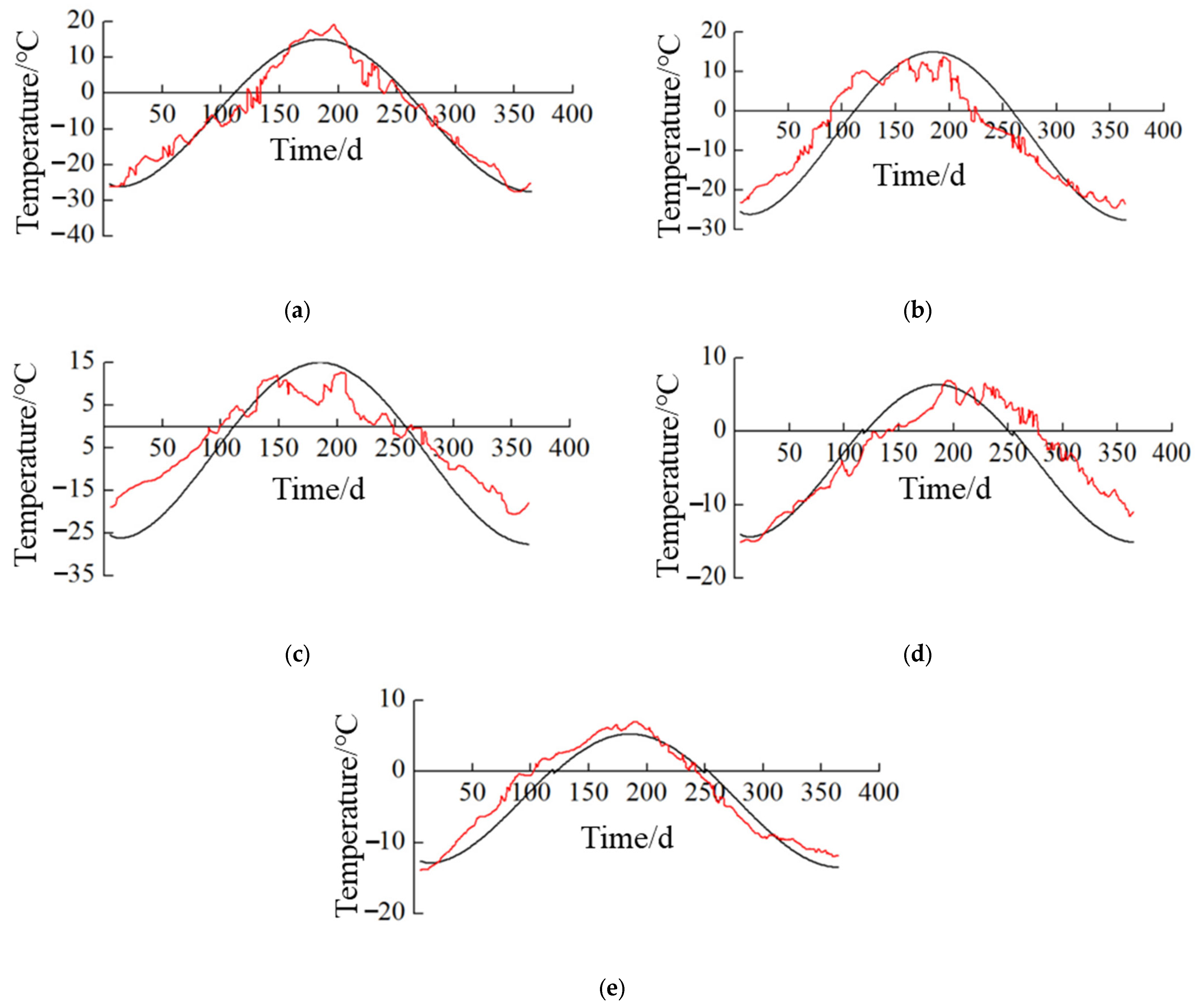
- The fluid–structure interaction calculation model of tunnels in cold regions is used to simulate the temperature field of 680 m at the portal section of the Hekashan tunnel and then compared with the measured data. It is found that the calculated value is basically consistent with the measured value over time, which indicates that the fluid–structure interaction model established in this paper has certain reliability.
- (4)
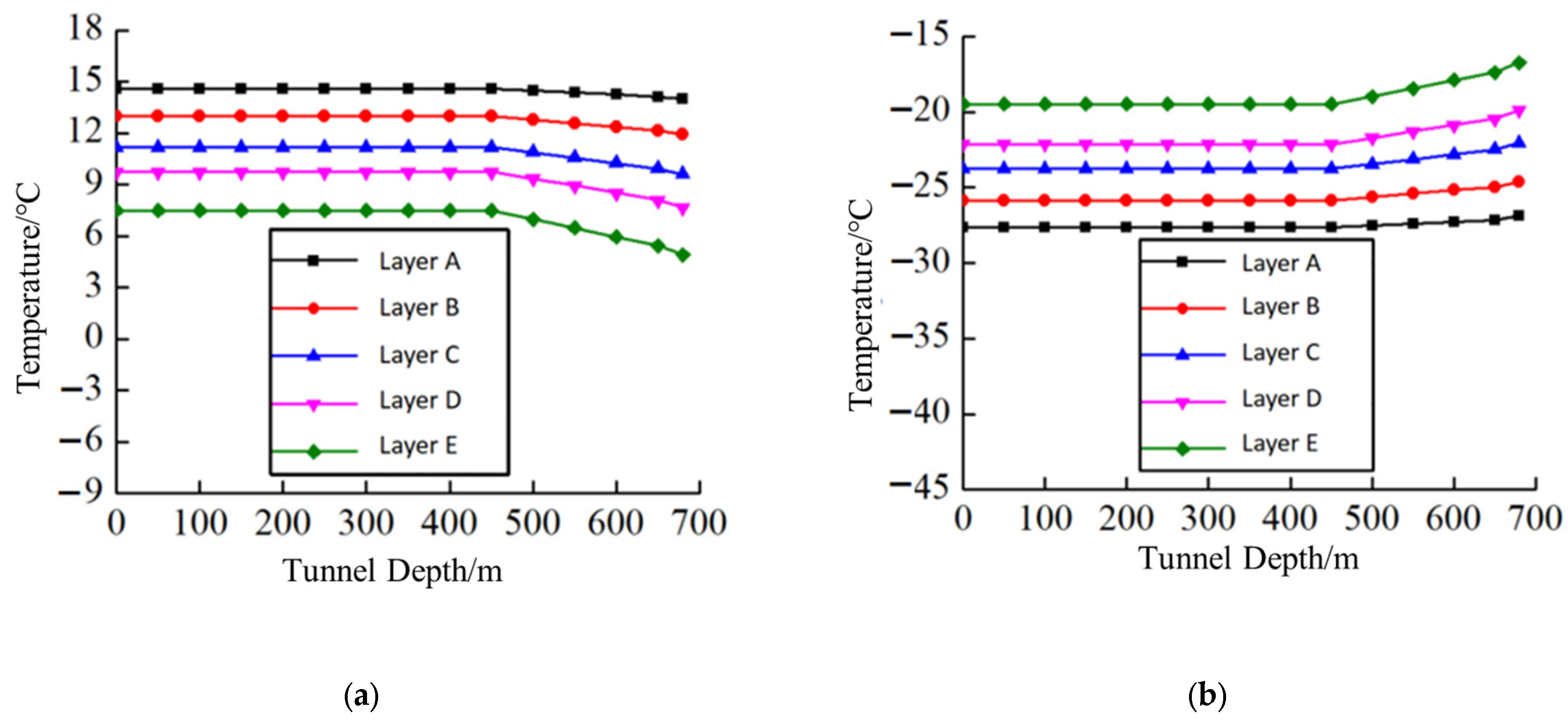
- Temperature monitoring points were set up in the sections of 0 m, 200 m, 400 m, 600 m, and 680 m of the secondary lining of the Hekashan tunnel. The measured temperature curves of each section of the secondary lining of the tunnel were obtained by averaging the five monitoring data of the left and right arch foot, the left and right arch waist, and the vault. It is found that the temperature of each layer of the tunnel lining changes in a sine curve with time, and the temperature of each layer gradually lags behind. The temperature variation amplitude of the extreme value of the layer temperature gradually decreases with the increase in the radial distance of the lining. Near the entrance end of the tunnel, the temperature of each layer of lining remains unchanged, and the temperature gradually decreases or increases with the increase in the depth.
- (5)
- In this paper, the distribution law of the temperature field in tunnels in cold areas is studied, on the basis of which the stress–strain relationship between the surrounding rock and the lining of the tunnel can be further studied.
Author Contributions
Funding
Institutional Review Board Statement
Informed Consent Statement
Data Availability Statement
Acknowledgments
Conflicts of Interest
References
- Zhang, F.S.; Huang, L.K.; Yang, L.; Dontsov, E.; Weng, D.W.; Liang, H.B.; Yin, Z.R.; Tang, J.Z. Numerical investigation on the effect of depletion-induced stress reorientation on infill well hydraulic fracture propagation. Pet. Sci. 2022, 19, 296–308. [Google Scholar] [CrossRef]
- Zheng, Y.; He, R.; Huang, L.; Bai, Y.; Wang, C.; Chen, W.; Wang, W. Exploring the effect of engineering parameters on the penetration of hydraulic fractures through bedding planes in different propagation regimes. Comput. Geotech. 2022, 146, 104736. [Google Scholar] [CrossRef]
- Luo, H.; Xie, J.; Huang, L.; Wu, J.; Shi, X.; Bai, Y.; Fu, H.; Pan, B. Multiscale sensitivity analysis of hydraulic fracturing parameters based on dimensionless analysis method. Lithosphere 2022, 2022, 9708300. [Google Scholar] [CrossRef]
- Huang, L.; Liu, J.; Zhang, F.; Dontsov, E.; Damjanac, B. Exploring the influence of rock inherent heterogeneity and grain size on hydraulic fracturing using discrete element modeling. Int. J. Solids Struct. 2019, 176, 207–220. [Google Scholar] [CrossRef]
- Huang, L.; Liu, J.; Ji, Y.; Gong, X.; Qin, L. A review of multiscale expansion of low permeability reservoir cracks. Petroleum 2018, 4, 115–125. [Google Scholar] [CrossRef]
- Han, Y.; Fu, Z.; Li, B. Heat Transfer Model and Temperature Field Distribution Law of Tunnel in Permafrost Region. China J. Highw. Transp. 2019, 32, 136–145. [Google Scholar]
- Xia, C.; Fan, D.; Han, C. Piecewise Calculation Method for Insulation Layer Thickness in Cold Region Tunnels. China J. Highw. Transp. 2013, 26, 131–139. [Google Scholar]
- Zhou, X.; Zeng, Y.; Yang, Z.; Yang, C.; Fang, W. Discussion of anti-freeze and frost resistance of shallow buried tunnels in high latitude cold region. J. Glaciol. Geocryol. 2016, 38, 121–128. [Google Scholar]
- Gao, Y.; Zhu, Y.; Zhao, D. Study on classified suggestion of tunnel in cold region and thermal insulation-considered drainage technology. Chin. J. Rock Mech. Eng. 2018, 37, 3489–3499. [Google Scholar]
- Yu, L.; Sun, Y.; Wang, M.; Xia, P.; Wang, G. Model and Action Law of Temperature Field of Tunnel in Cold Region Considering Ventilation and Surrounding Rock Condition. Tunn. Constr. 2019, 39, 85–91. [Google Scholar]
- Sun, K.; Xu, Y.; Chou, W.; Zheng, Q. On Temperature Field Distribution and the Effects of Surrounding Rock Properties on Tunnels in Cold Regions. Mod. Tunn. Technol. 2016, 53, 67–72. [Google Scholar]
- Sun, K.; Liu, J.; Yu, M. Influence law of meteorological elements on radialtemperature field of tunnel in a cold region. China Civ. Eng. J. 2021, 54, 140–148. [Google Scholar]
- Gao, Y.; Wang, M. Analysis on Air of Tunnel in Qilian Mountain and Temperature Field of Surrounding Rock. Sci. Technol. Eng. 2018, 18, 120–126. [Google Scholar]
- Zhou, X.; Zeng, Y.; Fan, L.; Zhou, X. Temporal-Spatial Evolution Laws of Temperature Field in Cold Region Tunnel and Temperature Control Measures. China Railw. Sci. 2016, 37, 46–52. [Google Scholar]
- Zhang, Y.; Xie, Y.; Li, Y.; Lai, J. A frost heave model based on space-time distribution of temperature field in cold region tunnels. Rock Soil Mech. 2018, 39, 1625–1632. [Google Scholar]
- Zhang, Y.; Song, Z.; Lai, J.; Li, Y. Spatial-temporal Distribution of 3D Temperature Field of Highway Tunnel in Seasonal Frozen Soil Region. J. Highw. Transp. Res. Dev. 2020, 37, 96–103. [Google Scholar]
- Zhang, Z.; Wang, S.; Yang, T.; Zhang, Y. Numerical Analysis on Hydro Thermal Coupling of Surrounding Rocks in Cold Region Tunnels. J. Northeast. Univ. Nat. Sci. 2020, 41, 635–641. [Google Scholar]
- Yu, J.; Wang, Z.; Jiang, X. Research on the Influence of Heat Transfer Coefficient and Surrounding Rock Conditions on Temperature Field in Cold Region Tunnel. J. Railw. Eng. Soc. 2021, 38, 40–47. [Google Scholar]
- Ma, C.; Li, Z.; Qiu, J. Freezing characteristics and freezing depth prediction of tunnels in cold regions. Tunn. Constr. 2023, 1–11. Available online: http://www.suidaojs.com/CN/abstract/abstract14190.shtml (accessed on 8 August 2023).
- Ding, Y.; Gao, Y.; Bao, X. Measurement and analysis of temperature field in Caomugou tunnel. Sci. Technol. Eng. 2022, 22, 5051–5059. [Google Scholar]
- Ma, J.; Chen, J.; Chen, W.; Huang, L. A coupled thermal-elastic-plastic-damage model for concrete subjected to dynamic loading. Int. J. Plast. 2022, 153, 103279. [Google Scholar] [CrossRef]
- Ma, J.; Chen, J.; Chen, W.; Liu, C.; Chen, W. A bounding surface plasticity model for expanded polystyrene-sand mixture. Transp. Geotech. 2022, 32, 100702. [Google Scholar] [CrossRef]
- Han, D.; Li, K. Physico-mechanical properties and brittle to plastic transition of a thermally cracked marble under uniaxial tension. Geothermics 2023, 109, 102642. [Google Scholar] [CrossRef]
- Huang, L.; Tan, J.; Fu, H.; Liu, J.; Chen, X.; Liao, X.; Wang, X.; Wang, C. The non-plane initiation and propagation mechanism of multiple hydraulic fractures in tight reservoirs considering stress shadow effects. Eng. Fract. Mech. 2023, 292, 109570. [Google Scholar] [CrossRef]
- Huang, L.; He, R.; Yang, Z.; Tan, P.; Chen, W.; Li, X.; Cao, A. Exploring hydraulic fracture behavior in glutenite formation with strong heterogeneity and variable lithology based on DEM simulation. Eng. Fract. Mech. 2023, 278, 109020. [Google Scholar] [CrossRef]
- Huang, L.; Dontsov, E.; Fu, H.; Lei, Y.; Weng, D.; Zhang, F. Hydraulic fracture height growth in layered rocks: Perspective from DEM simulation of different propagation regimes. Int. J. Solids Struct. 2022, 238, 111395. [Google Scholar] [CrossRef]
- Huang, L.; Liu, J.; Zhang, F.; Fu, H.; Zhu, H.; Damjanac, B. 3D lattice modeling of hydraulic fracture initiation and propagation for different perforation models. J. Pet. Sci. Eng. 2020, 191, 107169. [Google Scholar] [CrossRef]
- He, R.; Yang, J.; Li, L.; Yang, Z.; Chen, W.; Zeng, J.; Liao, X.; Huang, L. Investigating the simultaneous fracture propagation from multiple perforation clusters in horizontal wells using 3D block discrete element method. Front. Earth Sci. 2023, 11, 1115054. [Google Scholar] [CrossRef]
- Ma, J.; Ding, W.; Lin, Y.; Chen, W.; Huang, L. A fast and efficient particle packing generation algorithm with controllable gradation for discontinuous deformation analysis. Geomech. Geophys. Geo-Energy Geo-Resour. 2023, 9, 97. [Google Scholar] [CrossRef]
- Ma, J.; Zhao, J.; Lin, Y.; Liang, J.; Chen, J.; Chen, W.; Huang, L. Study on Tamped Spherical Detonation-Induced Dynamic Responses of Rock and PMMA Through Mini-Chemical Explosion Tests and a Four-Dimensional Lattice Spring Model. Rock Mech. Rock Eng. 2023, 2023, 1–19. [Google Scholar] [CrossRef]
- Zhang, X.; Wang, C.; Yu, W.; Liu, Z. Three-dimensional nonlinear analysis for coupled problem of heat transfer of surrounding rock and heat convection between air in Fenghuo Mountain tunnel and surrounding rock. Chin. J. Geotech. Eng. 2005, 27, 1414–1420. [Google Scholar]
- Wang, D.G.; Wang, H.J.; Xiong, J.H.; Tham, L.G. Characteristic-based operator-splitting finite element method for Navier-Stokes equations. Sci. China Technol. Sci. 2011, 54, 2157–2166. [Google Scholar] [CrossRef]
- Shui, Q.; Wang, D. Numerical Simulation for Navier-stokes Equations by Projection/Characteristic-based Operator-splitting Finite Element Method. Chin. J. Theor. Appl. Mech. 2014, 46, 369–381. [Google Scholar]
- Beale, J.T.; Majda, A. Rates of convergence for viscous splitting of the Navier-Stokes equations. Math. Comput. 1981, 37, 243–259. [Google Scholar] [CrossRef]
- Hundsdorfer, W.; Mozartova, A.; Spijker, M.N. Stepsize Restrictions for Boundedness and Monotonicity of Multistep Methods. J. Sci. Comput. 2012, 50, 265–286. [Google Scholar] [CrossRef]
- Zienkiewicz, O.C.; Taylor, R.L. The Element Method. Volume Three, Hydrodynamics; Tsinghua University: Beijing, China, 2008. [Google Scholar]
- Deng, G. Invesigation of Frost Protection Design for Tunnels in High Altitude Cold Regions; Southwest Jiaotong University: Chengdu, China, 2013. [Google Scholar]


| Elevation above Sea Level (m) | Average Temperature of Coldest Month (°C) | Length of Insulation Section (m) |
|---|---|---|
| 3300 | −10 | 680 |
| 3600 | −10.5 | 690 |
| 3800 | −11 | 710 |
| 4000 | −12 | 750 |
| 4200 | −13 | 830 |
| 4400 | −14 | 860 |
| 4600 | −15 | 900 |
| 4800 | −16 | 930 |
| Parameter | Surrounding Rock | Primary Lining | Lining Concrete | Air in the Hole |
|---|---|---|---|---|
| Thermal conductivity λ (W/(m·°C)) | 3.50 | 1.70 | 1.85 | 2.30 × 10⁻² |
| Density ρ (kg/m3) | 2120 | 2300 | 2500 | 1.40 |
| Specific Heat Capacity c (J/(kg·°C)) | 877 | 950 | 970 | 1000 |
| Dynamic Viscosity μ (Pa/·s) | - | - | - | 1.82 × 10⁻⁵ |
| Research Location | Maximum Temperature (°C) | Occurring Time (d) | Minimum Temperature (°C) | Occurring Time (d) |
|---|---|---|---|---|
| Secondary lining A layer | 14.90 | 3 July | −27.63 | 31 Dec. |
| Secondary lining B layer | 13.52 | 6 July | −25.85 | 31 Dec. |
| Secondary lining C layer | 12.00 | 11 July | −23.77 | 31 Dec. |
| Secondary lining D layer | 10.85 | 14 July | −22.13 | 31 Dec. |
| Secondary lining E layer | 9.09 | 21 July | −19.48 | 31 Dec. |
Disclaimer/Publisher’s Note: The statements, opinions and data contained in all publications are solely those of the individual author(s) and contributor(s) and not of MDPI and/or the editor(s). MDPI and/or the editor(s) disclaim responsibility for any injury to people or property resulting from any ideas, methods, instructions or products referred to in the content. |
© 2023 by the authors. Licensee MDPI, Basel, Switzerland. This article is an open access article distributed under the terms and conditions of the Creative Commons Attribution (CC BY) license (https://creativecommons.org/licenses/by/4.0/).
Share and Cite
Huang, J.; Shui, Q.; Wang, D.; Shi, Y.; Pu, X.; Wang, W.; Mao, X. Study on Temperature Distribution Law of Tunnel Portal Section in Cold Region Considering Fluid–Structure Interaction. Sustainability 2023, 15, 14524. https://doi.org/10.3390/su151914524
Huang J, Shui Q, Wang D, Shi Y, Pu X, Wang W, Mao X. Study on Temperature Distribution Law of Tunnel Portal Section in Cold Region Considering Fluid–Structure Interaction. Sustainability. 2023; 15(19):14524. https://doi.org/10.3390/su151914524
Chicago/Turabian StyleHuang, Jin, Qingxiang Shui, Daguo Wang, Yuhao Shi, Xiaosheng Pu, Wenzhe Wang, and Xuesong Mao. 2023. "Study on Temperature Distribution Law of Tunnel Portal Section in Cold Region Considering Fluid–Structure Interaction" Sustainability 15, no. 19: 14524. https://doi.org/10.3390/su151914524
APA StyleHuang, J., Shui, Q., Wang, D., Shi, Y., Pu, X., Wang, W., & Mao, X. (2023). Study on Temperature Distribution Law of Tunnel Portal Section in Cold Region Considering Fluid–Structure Interaction. Sustainability, 15(19), 14524. https://doi.org/10.3390/su151914524