


Timetable Rescheduling Using Skip-Stop Strategy for Sustainable Urban Rail Transit


Abstract
:1. Introduction
2. Literature Review
3. Problem Statement
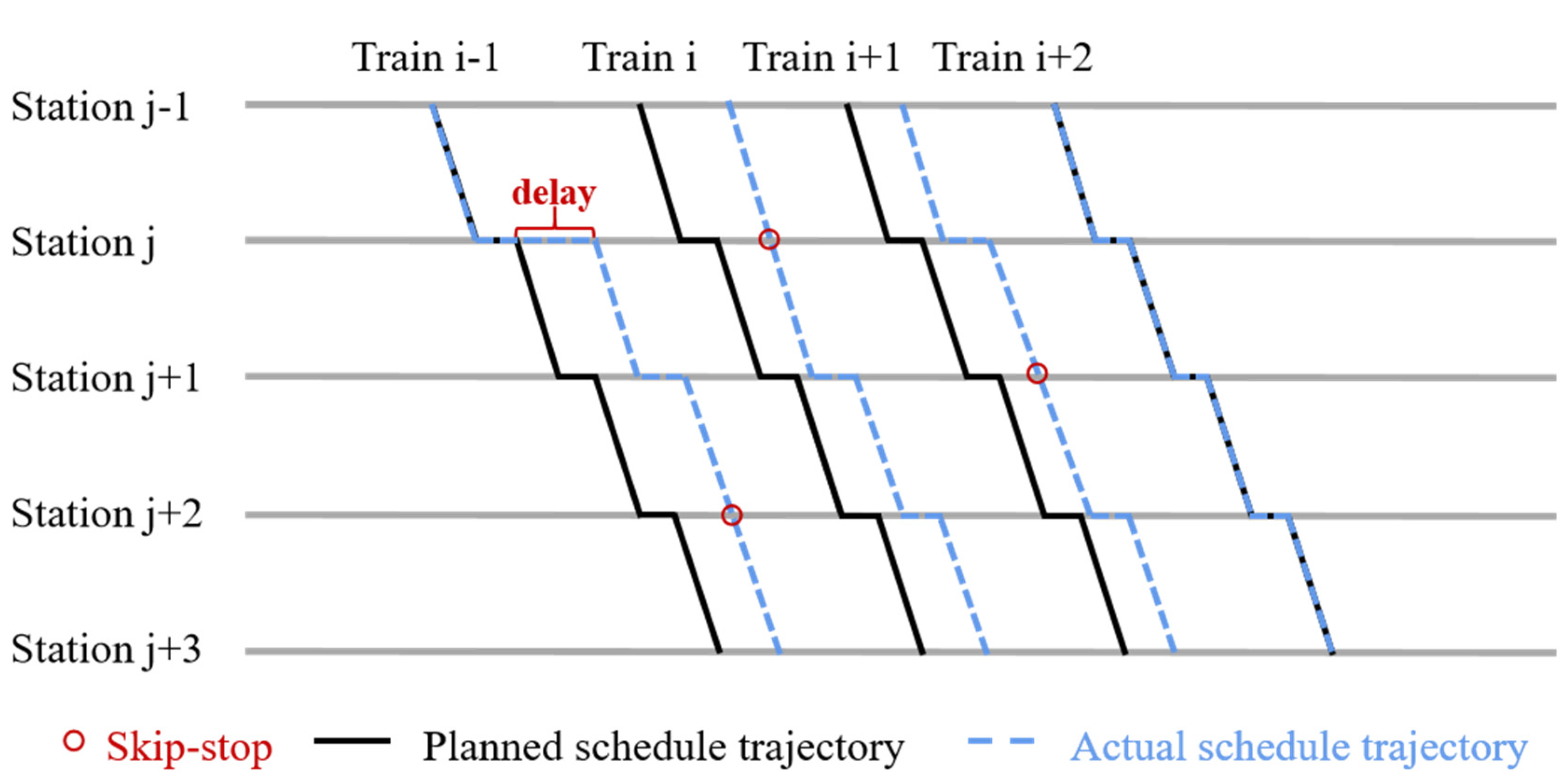
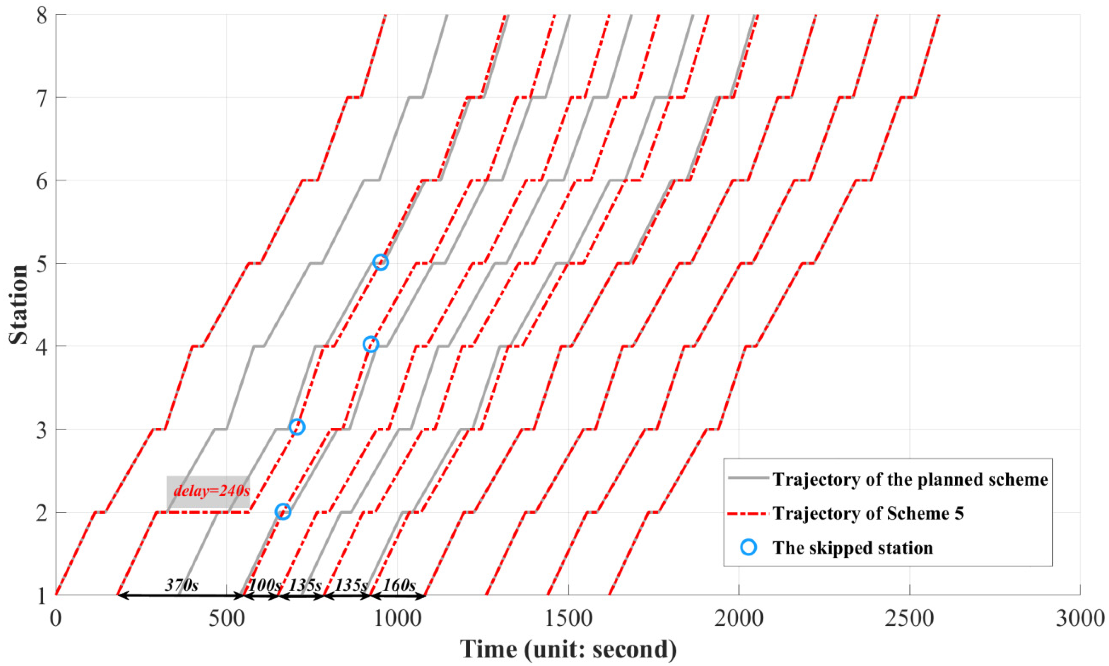
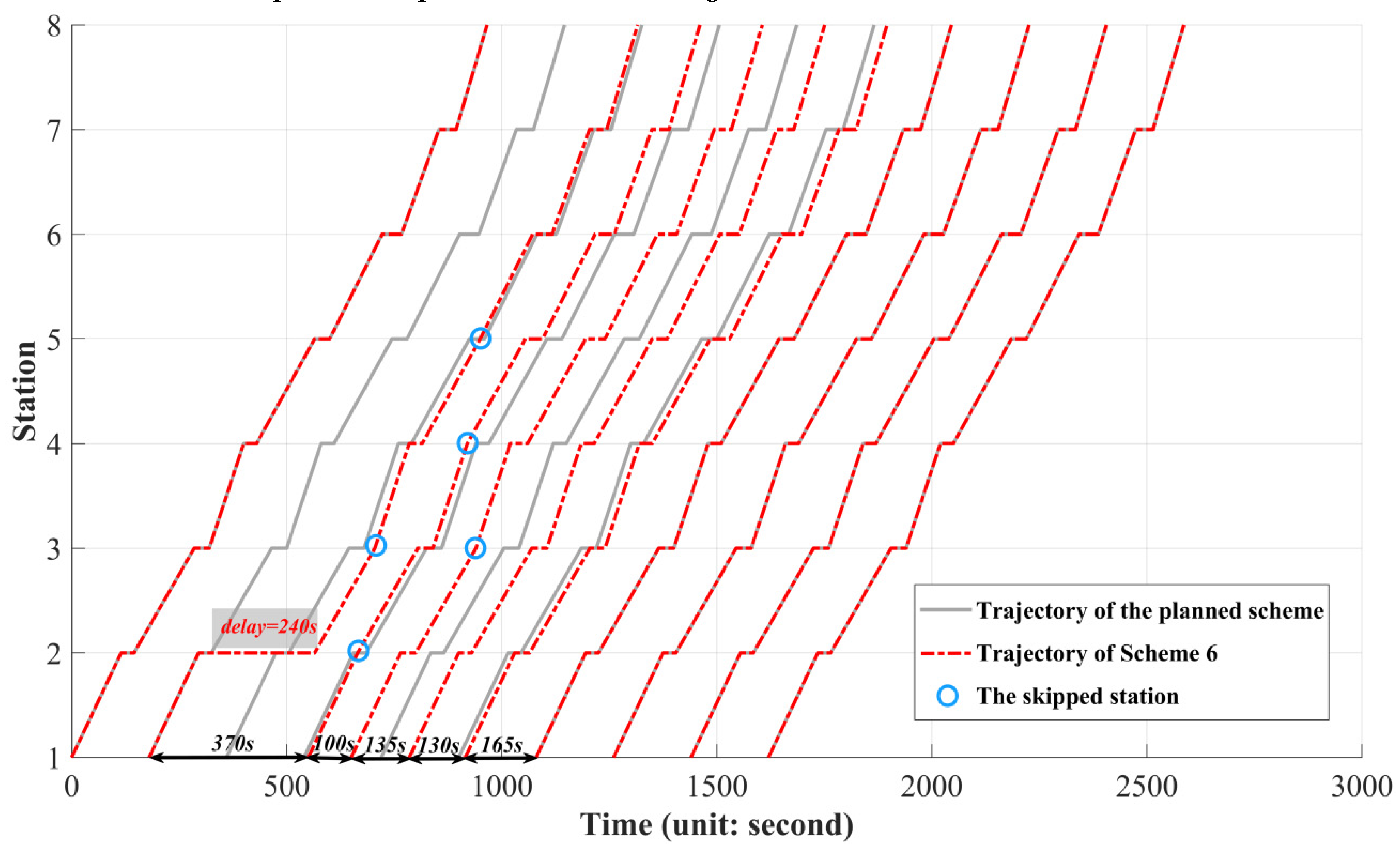
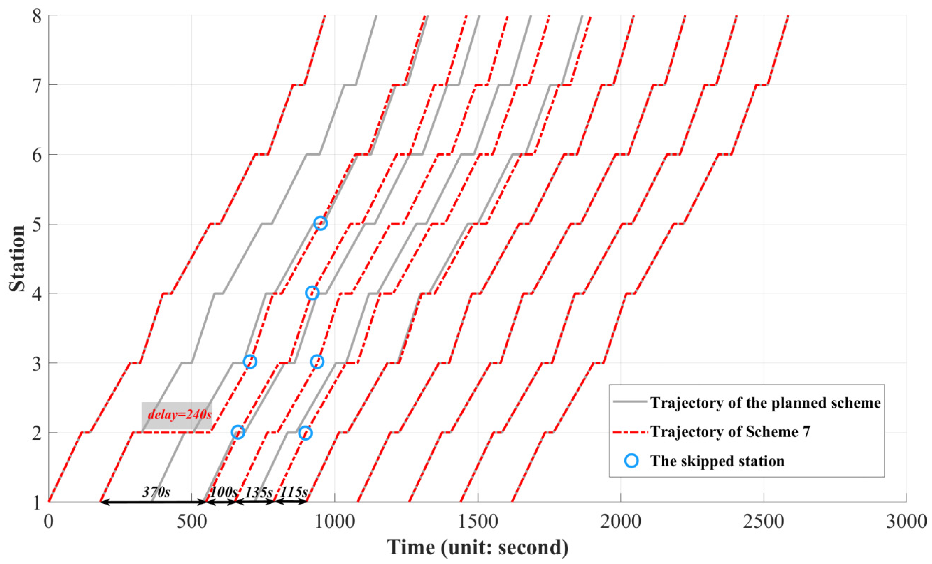
3.1. Skip-Stop Strategy
- Skip-stopping brings about potential time-saving benefits for passengers. By implementing this strategy, not only does it eradicate the time spent on train ’s dwelling at the skipped station but it also mitigates the need for the extra time allocated to the processes of acceleration and deceleration.
- Since some passengers whose boarding station is the skipped station , they cannot get on the train. As a result, they have to wait for the subsequent train to get on, increasing their waiting time.
- If destination station is skipped, some passengers cannot get off in time. These passengers have two choices in knowing the skip-stop information in advance. One is to get off at the previous station , then they need to spend extra time waiting for train to reach the end, and the other one is to get off at station , and then take the reverse train from it to the end [28,29,30].
3.2. Assumption
- Disruption events such as rail accidents, train breakdown, track damage, are not taken into account in this paper.
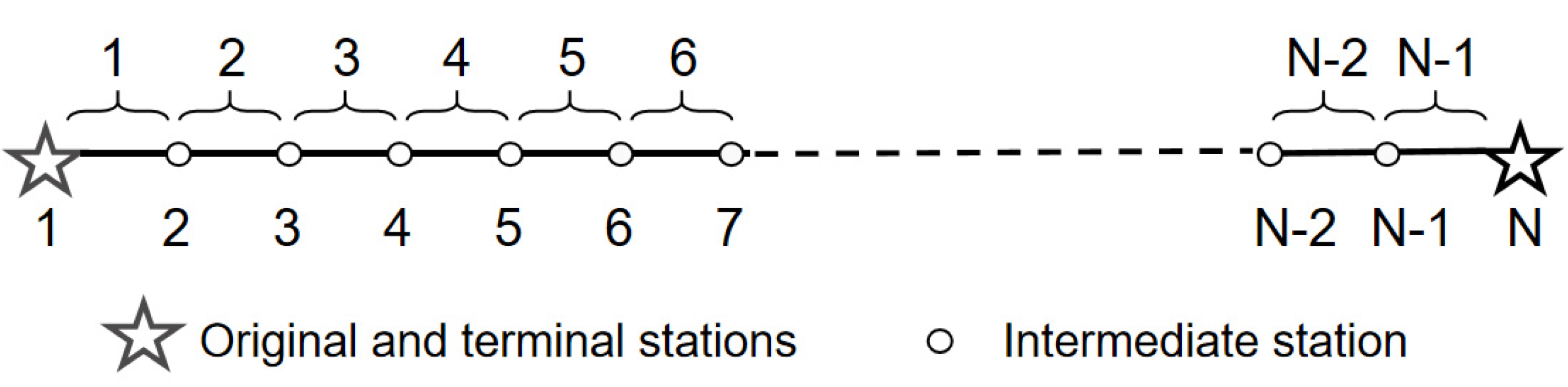
- Trains can adopt a flexible skip-stop operation to reschedule the planned timetable. However, the first and last stations are forbidden to be skipped. In addition, the train running time is fixed.
- Due to the unexpected train delay, it is imperative to account for the scenario in which trains have already commenced their journeys from station prior to the occurrence of the delay for train at the same station. Our model specifies that trains cannot change their timetables midway.
- Train k experiences an initial delay at station , and the subsequent trains need to wait at station and then operate based on the adjusted timetable.
- Utilizing the known passenger arrival rates, we conduct calculations to determine the passenger demand origin–destination (OD) for each station. Given the consistency of OD pairs during peak hours, it is reasonable to use these data as inputs for passenger demand.
3.3. Nomenclature
4. Formulation of the Model
4.1. Objective Functions
4.2. Constraints
4.2.1. Skip-Stop Constraint
4.2.2. Capacity-Based Passenger Loading Constraint
4.2.3. Timetabling Constraint
5. Solution Algorithm
5.1. Algorithm Applicability
5.2. Algorithm Framework
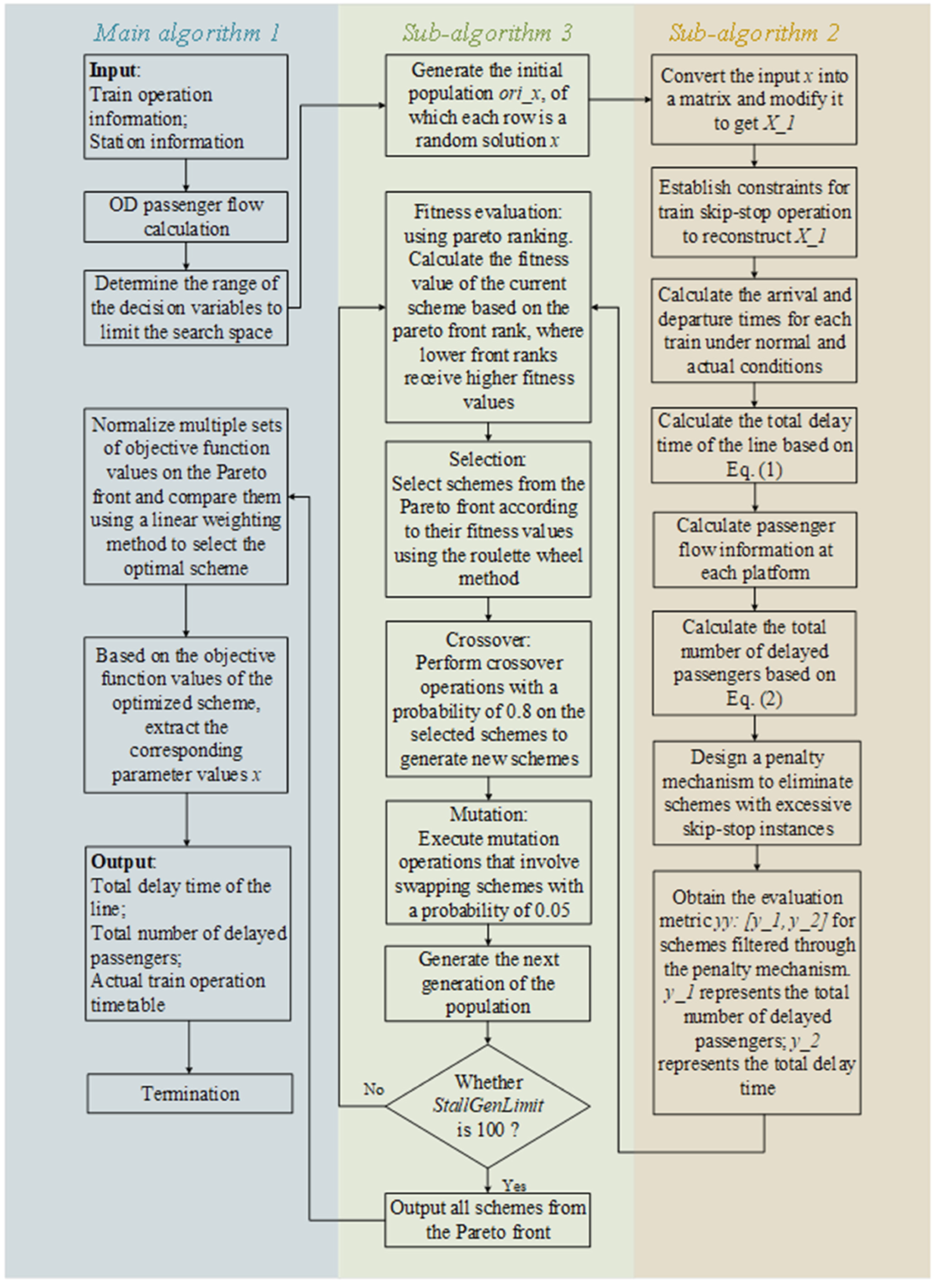
5.2.1. Main Algorithm 1
5.2.2. Sub-Algorithm 2
5.2.3. Sub-Algorithm 3
6. Case Study
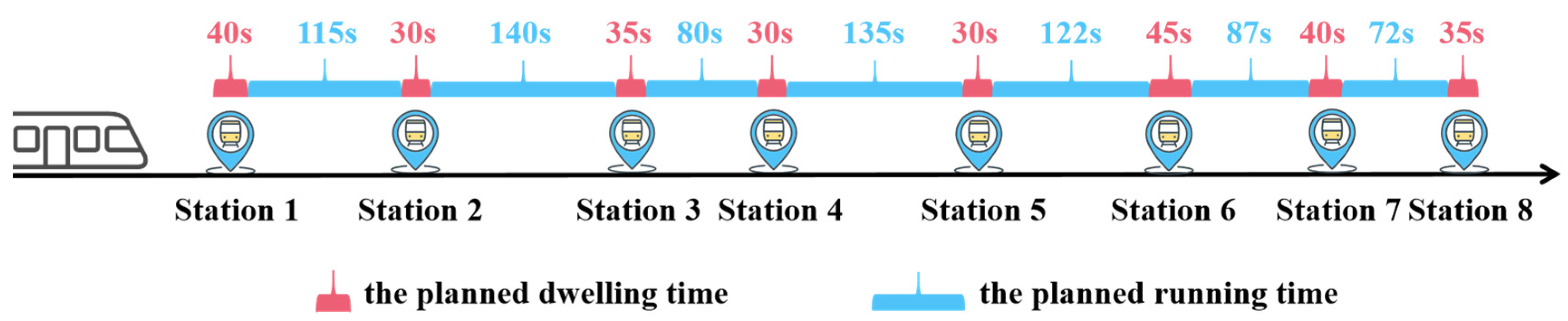
6.1. Data and Parameter Set
6.2. Computation Results
6.3. Comparisons for WOA and ECM
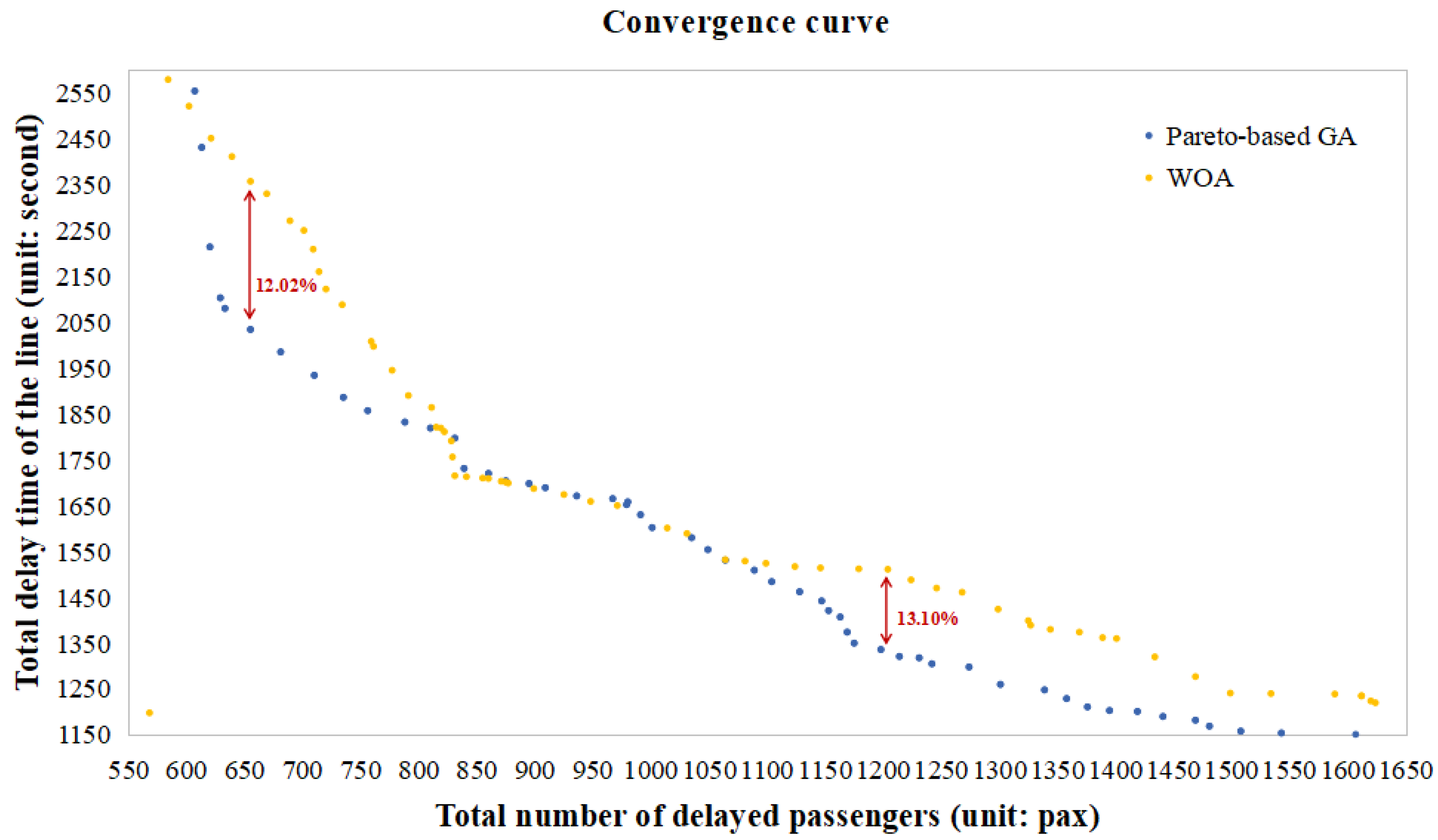
6.3.1. Comparison between Pareto-Based GA and WOA
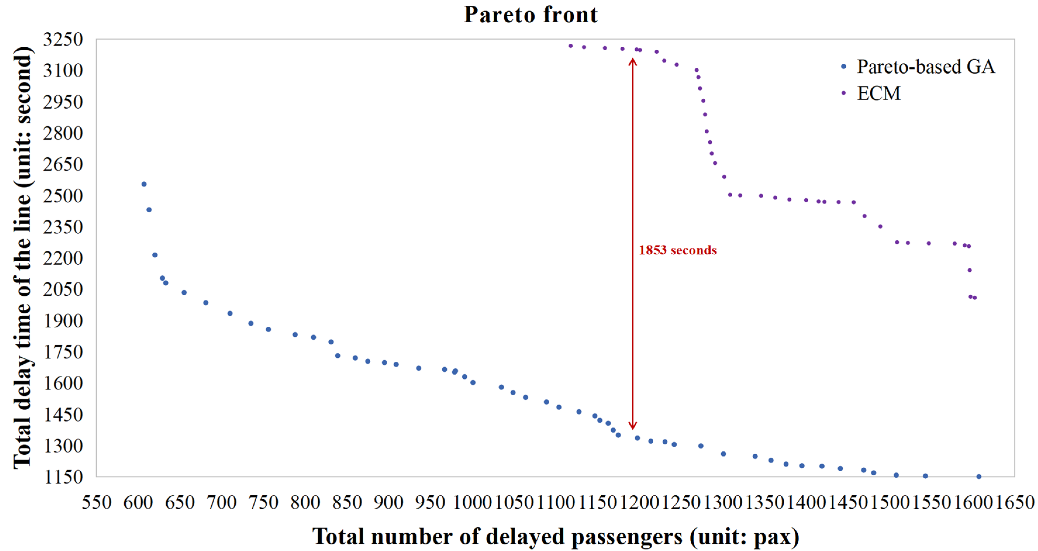
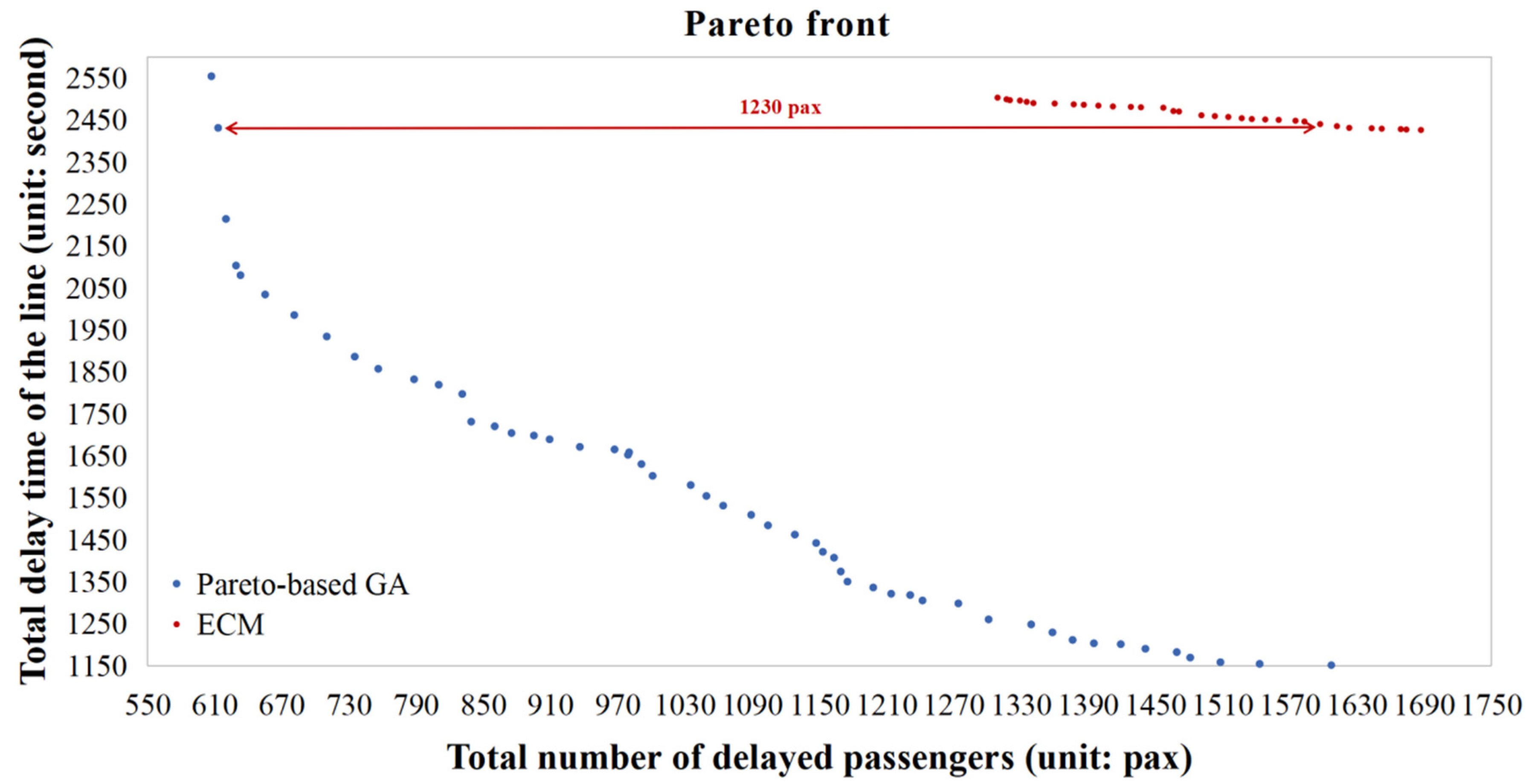
6.3.2. Comparison between Pareto-Based GA and ECM
6.4. Sensitivity Analysis
6.4.1. The Scheduled Headway
6.4.2. Penalty Coefficient
7. Conclusions
- (1)
- Investigate the formulation of skip-stop schemes under dynamic passenger flows to improve the accuracy of the model.
- (2)
- Extend the study to larger and more intricate transit networks, which can help evaluate the scalability and application of the proposed model in various contexts.
- (3)
- Incorporate external factors, such as weather conditions, unexpected incidents, and infrastructural constraints, into the optimization model to enhance its robustness and effectiveness in real-world scenarios.
Author Contributions
Funding
Institutional Review Board Statement
Informed Consent Statement
Data Availability Statement
Conflicts of Interest
References
- Huang, Q.; Jia, B.; Jiang, R.; Qiang, S. Simulation-based optimization in a bidirectional A/B skip-stop bus service. IEEE Access 2017, 5, 15478–15489. [Google Scholar] [CrossRef]
- Nesheli, M.M.; Ceder, A.A. Optimal combinations of selected tactics for public-transport transfer synchronization. Transp. Res. Part C Emerg. Technol. 2014, 48, 491–504. [Google Scholar] [CrossRef]
- Abdelhafiez, E.A.; Salama, M.R.; Shalaby, M.A. Minimizing passenger travel time in URT system adopting skip-stop strategy. J. Rail Transp. Plan. Manag. 2017, 7, 277–290. [Google Scholar] [CrossRef]
- Zhang, P.; Sun, Z.; Liu, X. Optimized skip-stop metro line operation using smart card data. J. Adv. Transp. 2017, 2017, 3097681. [Google Scholar] [CrossRef]
- Naeini, H.M.; Shafahi, Y.; SafariTaherkhani, M. Optimizing and synchronizing timetable in an urban subway network with stop-skip strategy. J. Rail Transp. Plan. Manag. 2022, 22, 100301. [Google Scholar]
- Cao, Z.; Yuan, Z.; Li, D. Estimation method for a skip-stop operation strategy for urban rail transit in China. J. Mod. Transp. 2014, 22, 174–182. [Google Scholar] [CrossRef]
- Li, Z.; Rui, S.; Shiwei, H.; Haodong, L. Optimization model and algorithm of skip-stop strategy for urban rail transit. J. China Railw. 2009, 31, 1–8. [Google Scholar]
- Gao, Y.; Kroon, L.; Schmidt, M.; Yang, L. Rescheduling a metro line in an over-crowded situation after disruptions. Transp. Res. Part B Methodol. 2016, 93, 425–449. [Google Scholar] [CrossRef]
- Shang, P.; Li, R.; Liu, Z.; Yang, L.; Wang, Y. Equity-oriented skip-stopping schedule optimization in an oversaturated urban rail transit network. Transp. Res. Part C Emerg. Technol. 2018, 89, 321–343. [Google Scholar] [CrossRef]
- Pan, H.C.; Yu, J.; Liu, Z.G.; Chen, W.J. Optimal train skip-stop operation at urban rail transit transfer stations for nonrecurrent extreme passenger flow mitigation. J. Transp. Eng. Part A Syst. 2020, 146, 04020062. [Google Scholar] [CrossRef]
- Chen, Z.; Li, S.; D’Ariano, A.; Yang, L. Real-time optimization for train regulation and stop-skipping adjustment strategy of urban rail transit lines. Omega 2022, 110, 102631. [Google Scholar] [CrossRef]
- Altazin, E.; Dauzère-Pérès, S.; Ramond, F.; Tréfond, S. Rescheduling through stop-skipping in dense railway systems. Transp. Res. Part C Emerg. Technol. 2017, 79, 73–84. [Google Scholar] [CrossRef]
- Zhu, Y.; Goverde, R.M. Railway timetable rescheduling with flexible stopping and flexible short-turning during disruptions. Transp. Res. Part B Methodol. 2019, 123, 149–181. [Google Scholar] [CrossRef]
- Li, S.; Dessouky, M.M.; Yang, L.; Gao, Z. Joint optimal train regulation and passenger flow control strategy for high-frequency metro lines. Transp. Res. Part B Methodol. 2017, 99, 113–137. [Google Scholar] [CrossRef]
- Lu, W.; Zhang, H.; Guo, J.; Qin, Y.; Jia, L. Coordinated control of urban rail train skip-stopping and inbound passenger flow based on deep Q-network. In Proceedings of the 5th International Conference on Electrical Engineering and Information Technologies for Rail Transportation (EITRT) 2021, Qingdao, China, 22–24 October 2021; pp. 545–547. [Google Scholar]
- Meng, F.; Yang, L.; Lu, Y.; Guo, R. Collaborative optimization of urban rail transit operation and passenger flow control at stations using skip-stop pattern strategy. J. Transp. Syst. Eng. Inf. Technol. 2021, 21, 156. [Google Scholar]
- Gkiotsalitis, K. A dynamic stop-skipping model for preventing public transport overcrowding beyond the pandemic-imposed capacity levels. In Proceedings of the 2022 IEEE 25th International Conference on Intelligent Transportation Systems (ITSC), Macau, China, 8–12 October 2022; pp. 681–686. [Google Scholar]
- Ibarra-Rojas, O.J.; Giesen, R.; Rios-Solis, Y.A. An integrated approach for timetabling and vehicle scheduling problems to analyze the trade-off between level of service and operating costs of transit networks. Transp. Res. Part B Methodol. 2014, 70, 35–46. [Google Scholar] [CrossRef]
- Lee, Y.J.; Shariat, S.; Choi, K. Optimizing skip-stop rail transit stopping strategy using a genetic algorithm. J. Public Transp. 2014, 17, 135–164. [Google Scholar] [CrossRef]
- Niu, H.; Zhou, X.; Gao, R. Train scheduling for minimizing passenger waiting time with time-dependent demand and skip-stop patterns: Nonlinear integer programming models with linear constraints. Transp. Res. Part B Methodol. 2015, 76, 117–135. [Google Scholar] [CrossRef]
- Zhao, J.; Ye, M.; Yang, Z.; Xing, Z.; Zhang, Z. Operation optimizing for minimizing passenger travel time cost and operating cost with time-dependent demand and skip-stop patterns: Nonlinear integer programming model with linear constraints. Transp. Res. Interdiscip. Perspect. 2021, 9, 100309. [Google Scholar] [CrossRef]
- Deng, L.; Peng, Q.; Cai, L.; Zeng, J.; Bhatt, N.R. Multiobjective Collaborative Optimization Method for the Urban Rail Multirouting Train Operation Plan. J. Adv. Transp. 2023, 2023, 3897353. [Google Scholar] [CrossRef]
- Gunantara, N. A review of multi-objective optimization: Methods and its applications. Cogent Eng. 2018, 5, 1502242. [Google Scholar] [CrossRef]
- Dulebenets, M.A. A Diffused Memetic Optimizer for reactive berth allocation and scheduling at marine container terminals in response to disruptions. Swarm Evol. Comput. 2023, 80, 101334. [Google Scholar] [CrossRef]
- Fathollahi-Fard, A.M.; Tian, G.; Ke, H.; Fu, Y.; Wong, K.Y. Efficient Multi-objective Metaheuristic Algorithm for Sustainable Harvest Planning Problem. Comput. Oper. Res. 2023, 158, 106304. [Google Scholar] [CrossRef]
- Pasha, J.; Nwodu, A.L.; Fathollahi-Fard, A.M.; Tian, G.; Li, Z.; Wang, H.; Dulebenets, M.A. Exact and metaheuristic algorithms for the vehicle routing problem with a factory-in-a-box in multi-objective settings. Adv. Eng. Inform. 2022, 52, 101623. [Google Scholar] [CrossRef]
- Anderluh, A.; Nolz, P.C.; Hemmelmayr, V.C.; Crainic, T.G. Multi-objective optimization of a two-echelon vehicle routing problem with vehicle synchronization and ‘grey zone’customers arising in urban logistics. Eur. J. Oper. Res. 2021, 289, 940–958. [Google Scholar] [CrossRef]
- Rajabighamchi, F.; Hosein Hajlou, E.M.; Hassannayebi, E. A multi-objective optimization model for robust skip-stop scheduling with earliness and tardiness penalties. Urban Rail Transit 2019, 5, 172–185. [Google Scholar] [CrossRef]
- Yang, L.; Qi, J.; Li, S.; Gao, Y. Collaborative optimization for train scheduling and train stop planning on high-speed railways. Omega 2016, 64, 57–76. [Google Scholar] [CrossRef]
- Haitao, W.U.; Chenglong, H.; Shuangxi, L.I.; Huiwen, T.A.N. Optimization of skip-stop strategy for urban rail transit considering passenger flow aggregation risk. China Saf. Sci. J. 2022, 32, 157. [Google Scholar]
- Liu, Y.; Feng, X.; Yang, Y.; Ruan, Z.; Zhang, L.; Li, K. Solving urban electric transit network problem by integrating Pareto artificial fish swarm algorithm and genetic algorithm. J. Intell. Transp. Syst. 2022, 26, 253–268. [Google Scholar] [CrossRef]
- Vlachopanagiotis, T.; Grizos, K.; Georgiadis, G.; Politis, I. Public Transportation Network Design and Frequency Setting: Pareto Optimality through Alternating-Objective Genetic Algorithms. Future Transp. 2021, 1, 248–267. [Google Scholar] [CrossRef]
- Owais, M.; Alshehri, A. Pareto optimal path generation algorithm in stochastic transportation networks. IEEE Access 2020, 8, 58970–58981. [Google Scholar] [CrossRef]
- Zan, X.; Wu, Z.; Guo, C.; Yu, Z. A Pareto-based genetic algorithm for multi-objective scheduling of automated manufacturing systems. Adv. Mech. Eng. 2020, 12, 1687814019885294. [Google Scholar] [CrossRef]
- Han, Z.; Han, B.; Li, D.; Ning, S.; Yang, R.; Yin, Y. Train timetabling in rail transit network under uncertain and dynamic demand using advanced and adaptive NSGA-II. Transp. Res. Part B Methodol. 2021, 154, 65–99. [Google Scholar] [CrossRef]
- Cui, Y.; Yu, Q.; Wang, C. Headway Optimisation for Metro Lines Based on Timetable Simulation and Simulated Annealing. J. Adv. Transp. 2022, 2022, 7035214. [Google Scholar] [CrossRef]
- Yuan, Y.; Li, S.; Yang, L.; Gao, Z. Real-time optimization of train regulation and passenger flow control for urban rail transit network under frequent disturbances. Transp. Res. Part E Logist. Transp. Rev. 2022, 168, 102942. [Google Scholar] [CrossRef]


| Publication (Chronologically) | Problem | Number of Sub-Objectives | Objective(s) | Modelling Approach | Solution Algorithms |
|---|---|---|---|---|---|
| Zhang et al. [4] | Optimization | 1 | To minimize the mean passenger travel time | MINLP | Genetic algorithm |
| Cao et al. [6] | Optimization | 1 | To minimize the total passenger waiting time, travel time, and train operating time | MIP | A tabu search algorithm |
| Gao et al. [8] | Optimization | 2 | To minimize both the total travel time and the number of waiting passengers | MILP | A heuristic algorithm |
| Shang et al. [9] | Optimization | 1 | To minimize the overall cost of arcs chosen by all passengers | LP | Dijkstra and Bellman- Ford |
| Pan et al. [10] | Delay | 1 | To minimize the total passenger delay | BP | Genetic algorithm |
| Altazin et al. [12] | Disturbance | 2 | To minimize both recovery times and passengers’ waiting times | NLIP | Dynamic programming algorithm |
| Zhu et al. [13] | Optimization | 1 | To minimize the total passenger travel time | MIP | Nested genetic algorithm |
| Li et al. [14] | Disruption | 2 | To minimize deviations in both the timetable and headway | QP | The MPC (Model predictive control) algorithm |
| Meng et al. [16] | Optimization | 2 | To minimize both the train service time and the number of passengers experiencing delays | MINLP | Time reconstruction and big-M method (CPLEX) |
| This paper (2023) | Delay | 2 | To minimize both the total delay time and the number of passengers experiencing delays | MILP | Pareto-based genetic algorithm |
| Sets | |
|---|---|
| Parameters | |
| Sequence number of delayed train | |
| Sequence number of the station at which the train encounters a delay | |
| Time when the initial delay occurred | |
| O | Duration of the delay |
| Planned station halt duration for train at station | |
| Anticipated travel duration for train between station and station | |
| Planned time for train to arrive/depart at station | |
| Minimum headway of trains | |
| Planned headway | |
| Minimum arrival and departure interval for a train | |
| Train’s maximum capacity | |
| Allowable maximum number of skip-stop instances for all trains | |
| Additional time for train acceleration/deceleration (unit: sec) | |
| Passenger arrival rate of station (unit: pax/sec) | |
| Variables | |
| encountering a delay, otherwise 0 | |
| Decision variables | |
| A binary variable which holds a value of 1 when train i stops at station j, otherwise 0 | |
| Station | |||||||||
|---|---|---|---|---|---|---|---|---|---|
| Train | |||||||||
| — | 8:01:55 | 8:04:45 | 8:06:40 | 8:09:25 | 8:12:02 | 8:14:14 | 8:16:06 | ||
| 8:00:00 | 8:02:25 | 8:05:20 | 8:07:10 | 8:10:00 | 8:12:47 | 8:14:54 | — | ||
| — | 8:04:55 | 8:07:45 | 8:09:40 | 8:12:25 | 8:15:02 | 8:17:14 | 8:19:06 | ||
| 8:03:00 | 8:05:25 | 8:08:20 | 8:10:10 | 8:13:00 | 8:15:47 | 8:17:54 | — | ||
| — | 8:07:55 | 8:10:45 | 8:12:40 | 8:15:25 | 8:18:02 | 8:20:14 | 8:22:06 | ||
| 8:06:00 | 8:08:25 | 8:11:20 | 8:13:10 | 8:16:00 | 8:18:47 | 8:20:54 | — | ||
| — | 8:10:55 | 8:13:45 | 8:15:40 | 8:18:25 | 8:21:02 | 8:23:14 | 8:25:06 | ||
| 8:09:00 | 8:11:25 | 8:14:20 | 8:16:10 | 8:19:00 | 8:21:47 | 8:23:54 | — | ||
| — | 8:13:55 | 8:16:45 | 8:18:40 | 8:21:25 | 8:24:02 | 8:26:14 | 8:28:06 | ||
| 8:12:00 | 8:14:25 | 8:17:20 | 8:19:10 | 8:22:00 | 8:24:47 | 8:26:54 | — | ||
| — | 8:16:55 | 8:19:45 | 8:21:40 | 8:24:25 | 8:27:02 | 8:29:14 | 8:31:06 | ||
| 8:15:00 | 8:17:25 | 8:20:20 | 8:22:10 | 8:25:00 | 8:27:47 | 8:29:54 | — | ||
| — | 8:19:55 | 8:22:45 | 8:24:40 | 8:27:25 | 8:30:02 | 8:32:14 | 8:34:06 | ||
| 8:18:00 | 8:20:25 | 8:23:20 | 8:25:10 | 8:28:00 | 8:30:47 | 8:32:54 | — | ||
| — | 8:22:55 | 8:25:45 | 8:27:40 | 8:30:25 | 8:33:02 | 8:35:14 | 8:37:06 | ||
| 8:21:00 | 8:23:25 | 8:26:20 | 8:28:10 | 8:31:00 | 8:33:47 | 8:35:54 | — | ||
| — | 8:25:55 | 8:28:45 | 8:30:40 | 8:33:25 | 8:36:02 | 8:38:14 | 8:40:06 | ||
| 8:24:00 | 8:26:25 | 8:29:20 | 8:31:10 | 8:34:00 | 8:36:47 | 8:38:54 | — | ||
| — | 8:28:55 | 8:31:45 | 8:33:40 | 8:36:25 | 8:39:02 | 8:41:14 | 8:43:06 | ||
| 8:27:00 | 8:29:25 | 8:32:20 | 8:34:10 | 8:37:00 | 8:39:47 | 8:41:54 | — | ||
| Station | Passenger Arrival Rate (Unit: Pax/Sec) |
|---|---|
| 1.036 | |
| 0.953 | |
| 0.821 | |
| 0.593 | |
| 0.421 | |
| 0.234 | |
| 0.150 |
| Destination | ||||||||
|---|---|---|---|---|---|---|---|---|
| Origin | ||||||||
| 17 | 14 | 25 | 25 | 21 | 19 | 24 | ||
| — | 22 | 27 | 21 | 31 | 27 | 15 | ||
| — | — | 18 | 31 | 19 | 15 | 21 | ||
| — | — | — | 22 | 32 | 23 | 12 | ||
| — | — | — | — | 27 | 12 | 22 | ||
| — | — | — | — | — | 14 | 20 | ||
| — | — | — | — | — | — | 21 | ||
| Scheme | Number of the Skipped Stations of all Trains | Total Number of Delayed Passengers (Unit: Pax) | Total Delay Time of the Line (Unit: Second) | (Unit: $) | Saving Percentage |
|---|---|---|---|---|---|
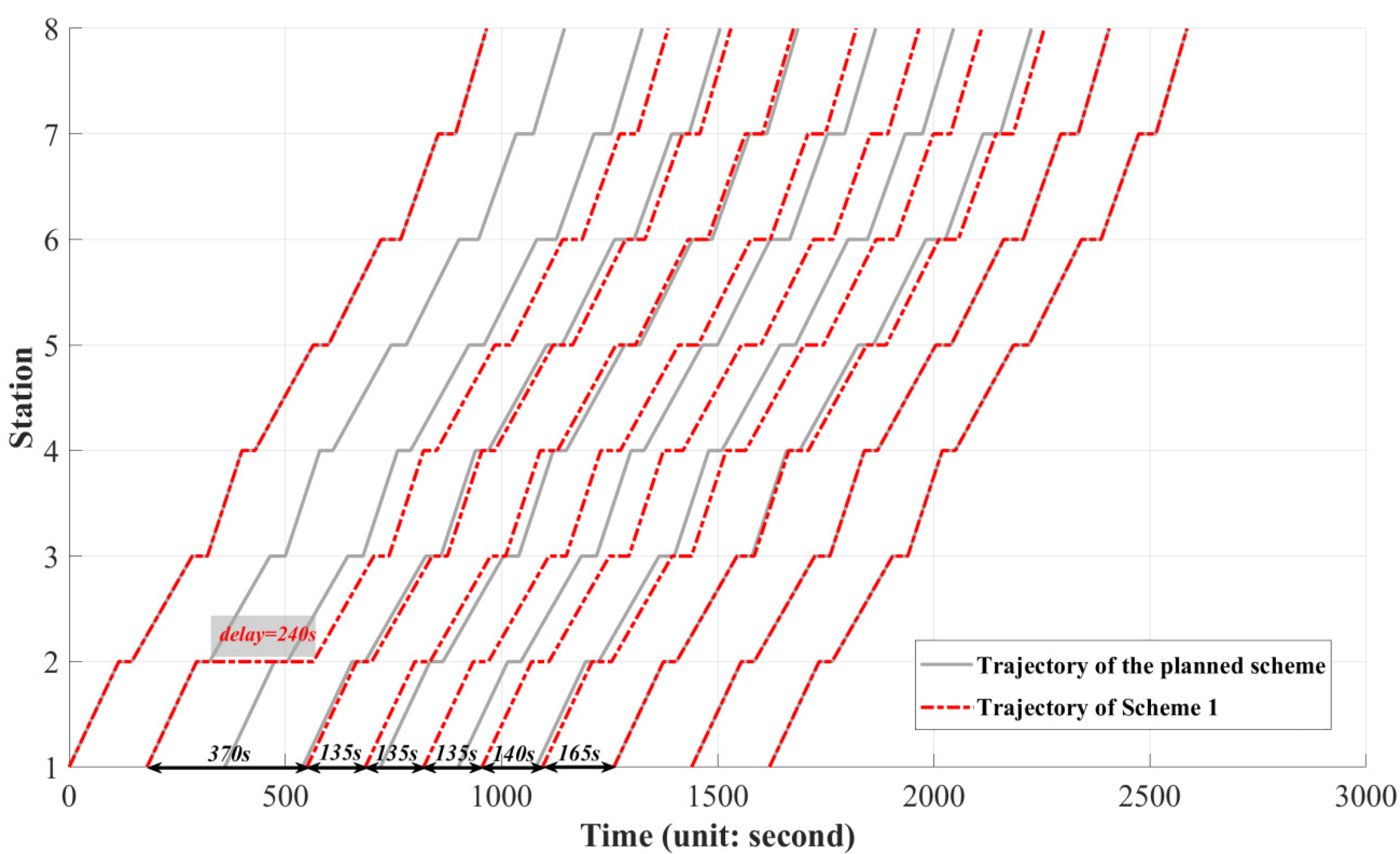
| 1 (basic) | 0 | 633 | 2080 | 2713 | — |
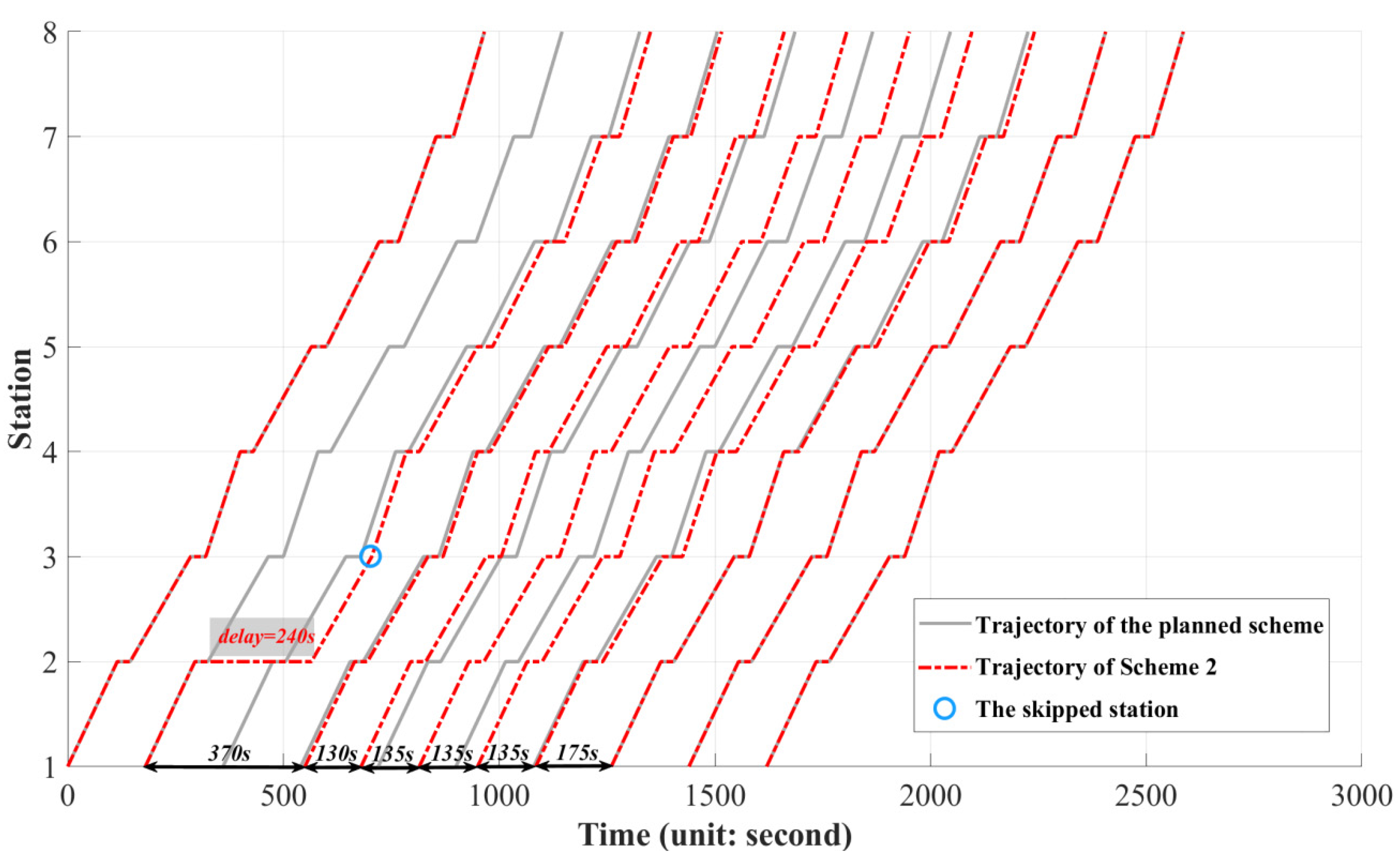
| 2 | 1 | 788 (↑24.49%) | 1832 (↓11.92%) | 2620 | 3.43% |
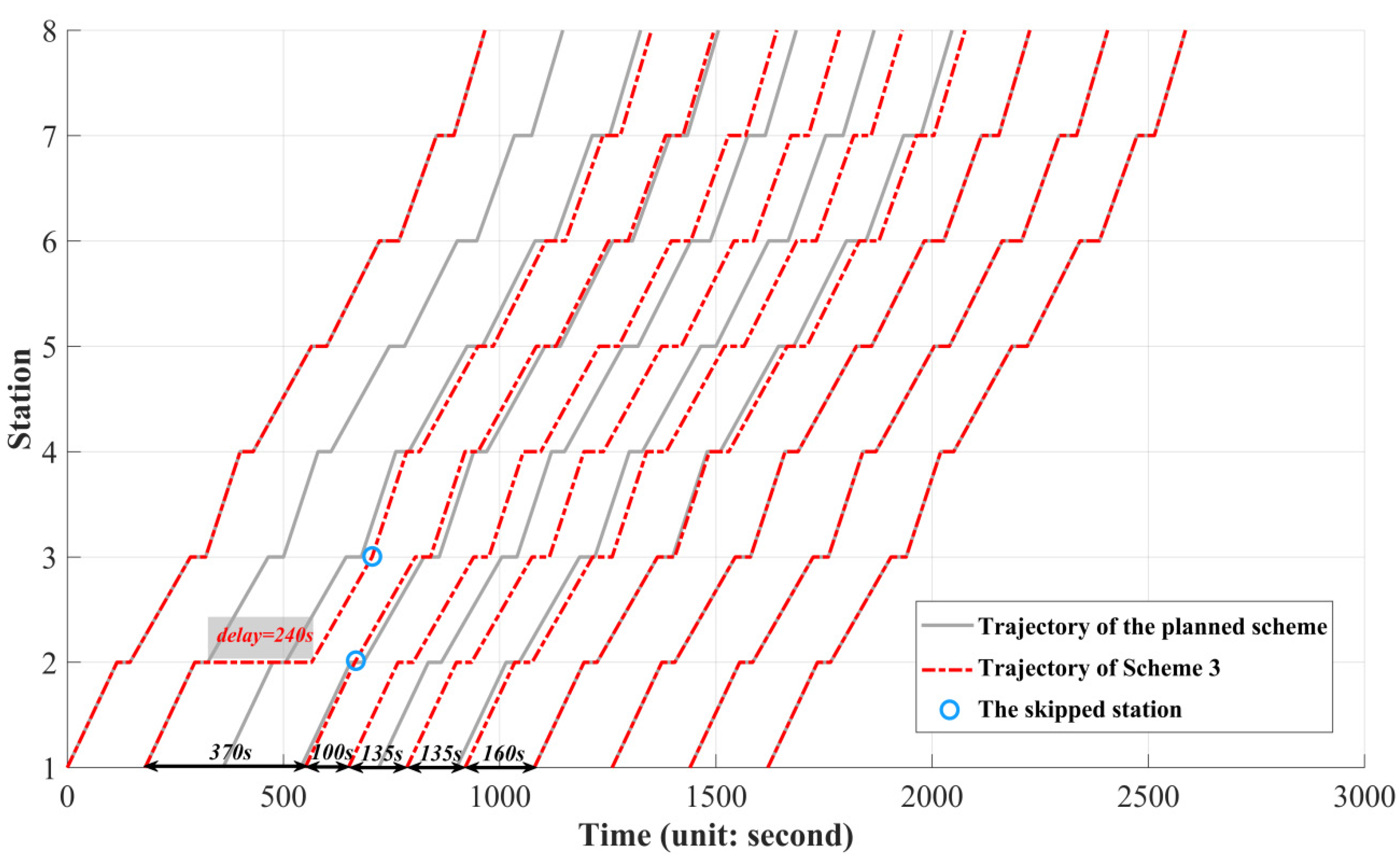
| 3 | 2 | 1064 (↑68.09%) | 1532 (↓26.35%) | 2596 | 4.31% |
| 4 | 3 | 1163 (↑83.73%) | 1407 (↓32.36%) | 2570 | 5.27% |
| 5 | 4 | 1242 (↑96.21%) | 1306 (↓37.21%) | 2548 (minimum) | 6.08% |
| 6 | 5 | 1395 (↑120.38%) | 1203 (↓42.16%) | 2598 | 4.24% |
| 7 | 6 | 1543 (↑143.76%) | 1154 (↓44.52%) | 2697 | 0.59% |
| Scheme | Trains Adjusting the Trajectory | Trains on Planned Trajectory |
|---|---|---|
| 1, 2 | 2, 3, 4, 5, 6, 7, 8 | 9, 10 |
| 3, 4, 5 | 2, 3, 4, 5, 6, 7 | 8, 9, 10 |
| 6, 7 | 2, 3, 4, 5, 6 | 7, 8, 9, 10 |
| Pareto-Based GA | WOA | ||||||||
|---|---|---|---|---|---|---|---|---|---|
| Scheme | Number of the Skipped Stations of all Trains | Total Number of Delayed Passengers (Unit: Pax) | Total Delay Time of the Line (Unit: Second) | (Unit: $) | CPU_Time (Unit: Second) | Total Number of Delayed Passengers (Unit: Pax) | Total Delay Time of the Line (Unit: Second) | (Unit: $) | CPU_Time (Unit: Second) |
| 1 | 0 | 633 | 2080 | 2713 | 150.14 | 568 | 1198 | 1766 (minimum) | 153.09 |
| 2 | 1 | 788 | 1832 | 2620 | 161.01 | 831 | 1768 | 2599 | 162.41 |
| 3 | 2 | 1064 | 1532 | 2596 | 195.62 | 1064 | 1532 | 2596 | 197.79 |
| 4 | 3 | 1163 | 1407 | 2570 | 215.20 | 1204 | 1511 | 2715 | 223.41 |
| 5 | 4 | 1242 | 1306 | 2548 (minimum) | 245.94 | 1317 | 1389 | 2706 | 257.54 |
| 6 | 5 | 1395 | 1203 | 2598 | 278.21 | 1327 | 1289 | 2616 | 298.24 |
| 7 | 6 | 1543 | 1154 | 2697 | 309.37 | 1612 | 1235 | 2847 | 341.05 |
(Unit: Second) | Total Number of Delayed Passengers (Unit: Pax) | Total Delay Time of the Line (Unit: Second) |
|---|---|---|
| 120 | 1642 (↑32.21%) | 5937 (↑354.59%) |
| 140 | 1731 (↑39.37%) | 4201 (↑221.67%) |
| 160 | 1862 (↑49.92%) | 2465 (↑88.74%) |
| 180 (basic) | 1242 | 1306 |
| 200 | 1599 (↑28.74%) | 923 (↓29.33%) |
| 220 | 1707 (↑37.44%) | 746 (↓42.88%) |
| 240 | 2066 (↑66.34%) | 615 (↓52.91%) |
| Scenario | Scheme | ($) | ($) | Saving Percentage | |
|---|---|---|---|---|---|
| 1 ) | 1 | 633 | 2080 | 2713 | — |
| 2 | 788 | 1832 | 2620 | 3.43% | |
| 3 | 1064 | 1532 | 2596 | 4.31% | |
| 4 | 1163 | 1407 | 2570 | 5.27% | |
| 5 | 1242 | 1306 | 2548 | 6.08% | |
| 6 | 1395 | 1203 | 2598 | 4.24% | |
| 7 | 1543 | 1154 | 2697 | 0.59% | |
| 2 ) | 1 | 633 | 20,800 | 21,433 | — |
| 2 | 788 | 18,320 | 19,108 | 10.85% | |
| 3 | 1064 | 15,320 | 16,384 | 23.56% | |
| 4 | 1163 | 14,070 | 15,233 | 28.93% | |
| 5 | 1242 | 13,060 | 14,302 | 33.27% | |
| 6 | 1395 | 12,030 | 13,425 | 37.36% | |
| 7 | 1543 | 11,540 | 13,083 | 38.96% | |
| 3 ) | 1 | 633 | 208,000 | 208,633 | — |
| 2 | 788 | 183,200 | 183,988 | 11.81% | |
| 3 | 1064 | 153,200 | 154,264 | 26.06% | |
| 4 | 1163 | 140,700 | 141,863 | 32.00% | |
| 5 | 1242 | 130,600 | 131,842 | 36.81% | |
| 6 | 1395 | 120,300 | 121,695 | 41.67% | |
| 7 | 1543 | 115,400 | 116,943 | 43.95% | |
| 4 ) | 1 | 6330 | 2080 | 8410 | 49.28% |
| 2 | 7880 | 1832 | 9712 | 41.44% | |
| 3 | 10,640 | 1532 | 12,172 | 26.60% | |
| 4 | 11,630 | 1407 | 13,037 | 21.39% | |
| 5 | 12,420 | 1306 | 13,726 | 17.23% | |
| 6 | 13,950 | 1203 | 15,153 | 8.63% | |
| 7 | 15,430 | 1154 | 16,584 | — | |
| 5 ) | 1 | 6330 | 20,800 | 27,130 | — |
| 2 | 7880 | 18,320 | 26,200 | 3.43% | |
| 3 | 10,640 | 15,320 | 25,960 | 4.31% | |
| 4 | 11,630 | 14,070 | 25,700 | 5.27% | |
| 5 | 12,420 | 13,060 | 25,480 | 6.08% | |
| 6 | 13,950 | 12,030 | 25,980 | 4.24% | |
| 7 | 15,430 | 11,540 | 26,970 | 0.59% | |
| 6 ) | 1 | 6330 | 208,000 | 214,330 | — |
| 2 | 7880 | 183,200 | 191,080 | 10.85% | |
| 3 | 10,640 | 153,200 | 163,840 | 23.56% | |
| 4 | 11,630 | 140,700 | 152,330 | 28.93% | |
| 5 | 12,420 | 130,600 | 143,020 | 33.27% | |
| 6 | 13,950 | 120,300 | 134,250 | 37.36% | |
| 7 | 15,430 | 115,400 | 130,830 | 38.96% | |
| 7 ) | 1 | 63,300 | 2080 | 65,380 | 57.92% |
| 2 | 78,800 | 1832 | 80,632 | 48.13% | |
| 3 | 106,400 | 1532 | 107,932 | 30.57% | |
| 4 | 116,300 | 1407 | 117,707 | 24.28% | |
| 5 | 124,200 | 1306 | 125,506 | 19.26% | |
| 6 | 139,500 | 1203 | 140,703 | 9.49% | |
| 7 | 154,300 | 1154 | 155,454 | — | |
| 8 ) | 1 | 63,300 | 20,800 | 84,100 | 49.28% |
| 2 | 78,800 | 18,320 | 97,120 | 41.44% | |
| 3 | 106,400 | 15,320 | 121,720 | 26.60% | |
| 4 | 116,300 | 14,070 | 130,370 | 21.39% | |
| 5 | 124,200 | 13,060 | 137,260 | 17.23% | |
| 6 | 139,500 | 12,030 | 151,530 | 8.63% | |
| 7 | 154,300 | 11,540 | 165,840 | — | |
| 9 ) | 1 | 63,300 | 208,000 | 271,300 | — |
| 2 | 78,800 | 183,200 | 262,000 | 3.43% | |
| 3 | 106,400 | 153,200 | 259,600 | 4.31% | |
| 4 | 116,300 | 140,700 | 257,000 | 5.27% | |
| 5 | 124,200 | 130,600 | 254,800 | 6.08% | |
| 6 | 139,500 | 120,300 | 259,800 | 4.24% | |
| 7 | 154,300 | 115,400 | 269,700 | 0.59% |
Disclaimer/Publisher’s Note: The statements, opinions and data contained in all publications are solely those of the individual author(s) and contributor(s) and not of MDPI and/or the editor(s). MDPI and/or the editor(s) disclaim responsibility for any injury to people or property resulting from any ideas, methods, instructions or products referred to in the content. |
© 2023 by the authors. Licensee MDPI, Basel, Switzerland. This article is an open access article distributed under the terms and conditions of the Creative Commons Attribution (CC BY) license (https://creativecommons.org/licenses/by/4.0/).
Share and Cite
Cao, Z.; Wang, Y.; Yang, Z.; Chen, C.; Zhang, S. Timetable Rescheduling Using Skip-Stop Strategy for Sustainable Urban Rail Transit. Sustainability 2023, 15, 14511. https://doi.org/10.3390/su151914511
Cao Z, Wang Y, Yang Z, Chen C, Zhang S. Timetable Rescheduling Using Skip-Stop Strategy for Sustainable Urban Rail Transit. Sustainability. 2023; 15(19):14511. https://doi.org/10.3390/su151914511
Chicago/Turabian StyleCao, Zhichao, Yuqing Wang, Zihao Yang, Changjun Chen, and Silin Zhang. 2023. "Timetable Rescheduling Using Skip-Stop Strategy for Sustainable Urban Rail Transit" Sustainability 15, no. 19: 14511. https://doi.org/10.3390/su151914511
APA StyleCao, Z., Wang, Y., Yang, Z., Chen, C., & Zhang, S. (2023). Timetable Rescheduling Using Skip-Stop Strategy for Sustainable Urban Rail Transit. Sustainability, 15(19), 14511. https://doi.org/10.3390/su151914511