
Risk Decision for a Port Shore Power Supply System Based on Cumulative Prospect Theory and an Improved Gray Target


Abstract
:1. Introduction
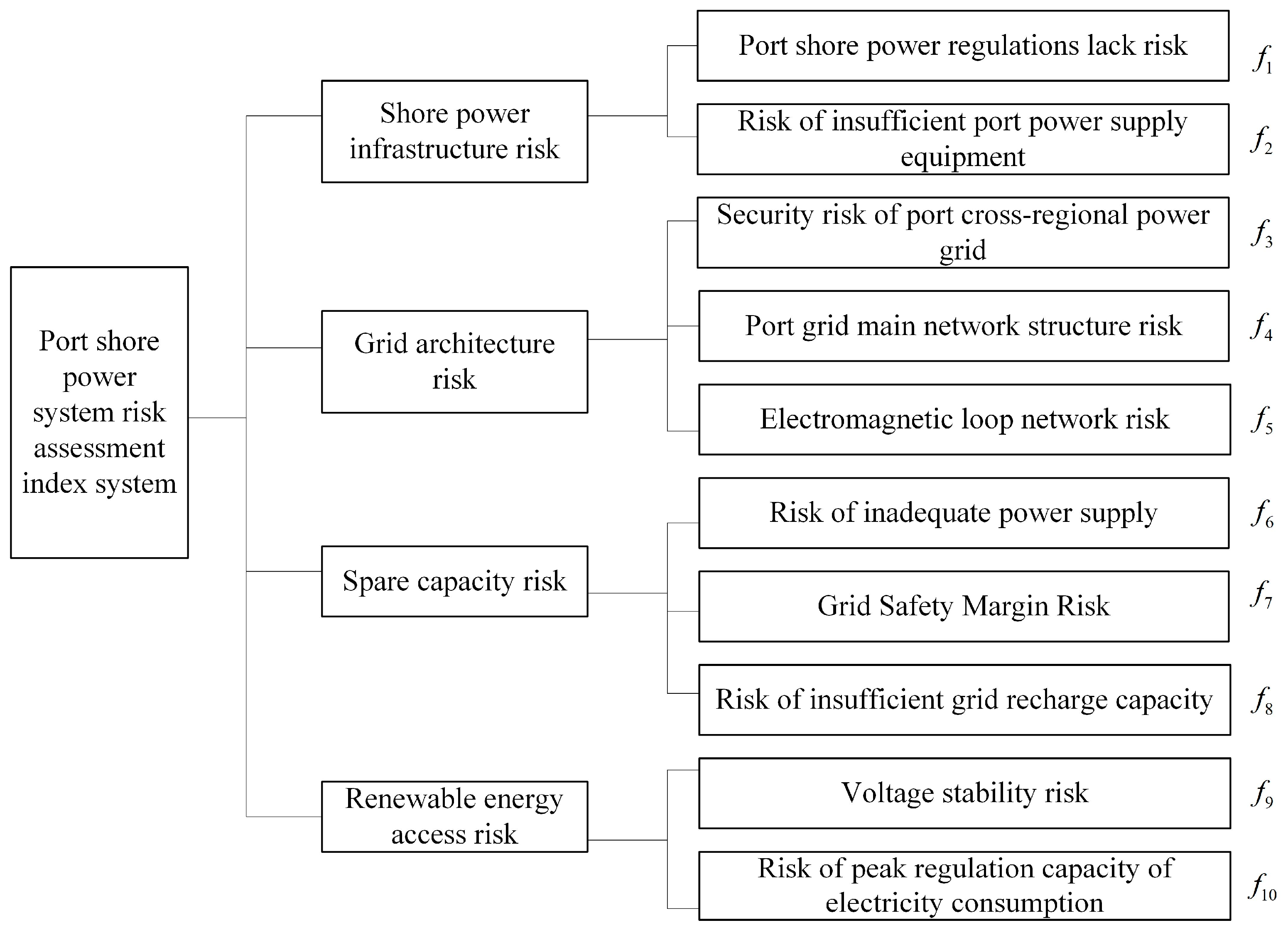
2. Indicator System
3. Methodology
3.1. Interval Gray Number
3.1.1. Interval Gray Nature
3.1.2. Comparison Rules for Interval Gray Numbers
3.2. Cumulative Prospect Theory
3.3. Improved Gray Target Decision Model
3.3.1. Positive and Negative Bullseye Distance and Bullseye Spacing
3.3.2. Comprehensive Judgment Distance
3.3.3. Improved Method for Determining Weights
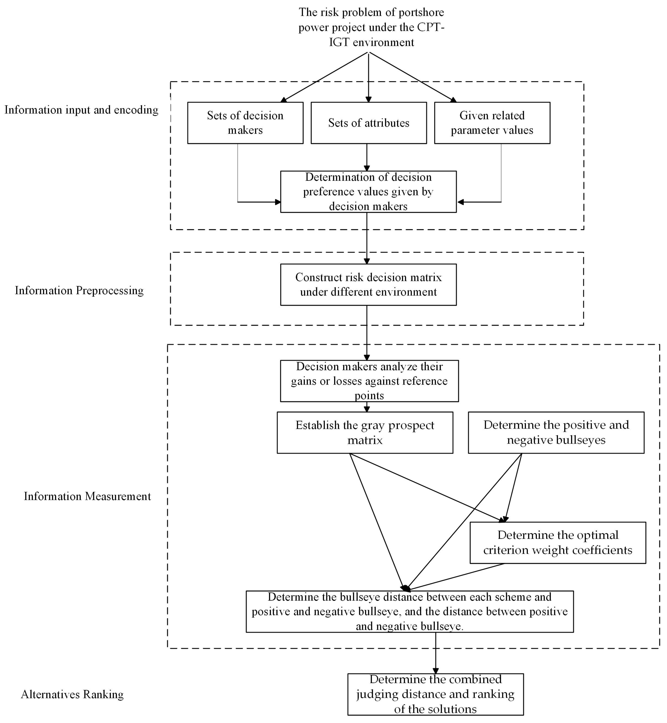
4. Model Design
4.1. Description of the Problem
4.2. Decision-Making Step
5. Case Study
5.1. An Illustrative Example about Port Shore Power Project Risk
5.2. Comparative Analysis
6. Conclusions
Author Contributions
Funding
Institutional Review Board Statement
Informed Consent Statement
Data Availability Statement
Conflicts of Interest
References
- Global Information. Available online: https://www.giiresearch.com/report/dmin1285071-global-shore-power-market.html (accessed on 17 August 2023).
- Sciberras, E.A.; Zahawi, B.; Atkinson, D.J. Electrical characteristics of cold ironing energy supply for berthed ships. Transp. Res. Part D 2015, 39, 31–43. [Google Scholar] [CrossRef]
- Ballini, F.; Bozzo, R. Air pollution from ships in ports: The socio-economic benefit of cold-ironing technology. Res. Transp. Bus. Manag. 2015, 17, 92–98. [Google Scholar] [CrossRef]
- Vaishnav, P.; Fischbeck, P.S.; Morgan, M.G.; Corbett, J.J. Shore power for vessels calling at US ports: Benefits and costs. Environ. Sci. Technol. 2016, 50, 1102–1110. [Google Scholar] [CrossRef] [PubMed]
- Winkel, R.; Weddige, U.; Johnsen, D.; Hoen, V.; Papaefthimiou, S. Shore side electricity in Europe: Potential and environmental benefits. Energy Policy 2016, 88, 584–593. [Google Scholar] [CrossRef]
- Kotrikla, A.M.; Lilas, T.; Nikitakos, N. Abatement of air pollution at an aegean island port utilizing shore side electricity and renewable energy. Mar. Policy 2017, 75, 238–248. [Google Scholar] [CrossRef]
- Innes, A.; Monios, J. Identifying the unique challenges of installing cold ironing at small and medium ports—The case of Aberdeen. Transp. Res. Part D 2018, 62, 298–313. [Google Scholar] [CrossRef]
- Zis, T.P. Prospects of cold ironing as an emissions reduction option. Transp. Res. Part A 2019, 119, 82–95. [Google Scholar] [CrossRef]
- Roberts, T.; Williams, I.; Preston, J.; Clarke, N.; Odum, M.; O’Gorman, S. Ports in a Storm: Port-City Environmental Challenges and Solutions. Sustainability 2023, 15, 9722. [Google Scholar] [CrossRef]
- He, Z.; Lam, J.S.L.; Liang, M. Impact of Disruption on Ship Emissions in Port: Case of Pandemic in Long Beach. Sustainability 2023, 15, 7215. [Google Scholar] [CrossRef]
- Antunes, T.A.; Castro, R.; Santos, P.J.; Pires, A.J. Standardization of Power-from-Shore Grid Connections for Offshore Oil & Gas Production. Sustainability 2023, 15, 5041. [Google Scholar]
- Li, C.; Chai, Y.; Qi, Z. Improved Grey Target Risk Decision Model in Smart Transmission System Based on Prospect Theory. Oper. Res. Manag. Sci. 2014, 3, 83–90. (In Chinese) [Google Scholar]
- Fekri, M.; Nikoukar, J.; Gharehpetian, G.B. Vulnerability risk assessment of electrical energy transmission systems with the approach of identifying the initial events of cascading failures. Electr. Power Syst. Res. 2023, 220, 109271. [Google Scholar] [CrossRef]
- Ding, T.; Li, C.; Yan, C.; Li, F.; Bie, Z. A bilevel optimization model for risk assessment and contingency ranking in transmission system reliability evaluation. IEEE Trans. Power Syst. 2016, 32, 3803–3813. [Google Scholar] [CrossRef]
- Niu, D.; Song, Z.; Wang, M.; Xiao, X. Improved TOPSIS method for power distribution network investment decision-making based on benefit evaluation indicator system. Int. J. Energy Sect. Manag. 2017, 11, 595–608. [Google Scholar] [CrossRef]
- González, J.S.; Payán, M.B.; Santos, J.R. Optimum design of transmissions systems for offshore wind farms including decision making under risk. Renew. Energy 2013, 59, 115–127. [Google Scholar] [CrossRef]
- Zhang, L.; Wu, J.; Zhang, J.; Su, F.; Bian, H.; Li, L. A dynamic and integrated approach of safety investment decision-making for power grid enterprises. Process Saf. Environ. Prot. 2022, 162, 301–312. [Google Scholar] [CrossRef]
- Kahneman, D.; Tversky, A. Prospect theory: An analysis of decision under risk. Economica 1979, 47, 263–291. [Google Scholar]
- Tversky, A.; Kahneman, D. Advances in prospect theory: Cumulative representation of uncertainty. J. Risk Uncertain. 1992, 5, 297–323. [Google Scholar] [CrossRef]
- Deng, J.L. Control problems of grey systems. Syst. Control Lett. 1982, 1, 288–294. [Google Scholar]
- Liu, S.F.; Lin, Y. Grey Information: Theory and Practical Applications; Springer: London, UK, 2006. [Google Scholar]
- Feng, J.Y.; Zhang, H. Grey target model appraising firms’ financial status based on altman coefficients. J. Grey Syst. 2006, 18, 133–142. [Google Scholar]
- Liu, S.X.; Cao, Y.D.; Hou, C.G.; Liu, X.; Li, J. Application of improved gray target theory based assessment on insulation state of solid-insulated ring main unit. J. Power Syst. Technol. 2013, 37, 3577–3583. [Google Scholar]
- Wang, B.; Tao, J.L.; Liu, D.F.; Chen, X.B. Dynamic evaluation model of networked manufacturing resources based on grey target decision. Inf. Technol. J. 2013, 12, 534. [Google Scholar]
- Jia, L.; Tong, Z.; Wang, C.; Li, S. Aircraft combat survivability calculation based on combination weighting and multiattribute intelligent grey target decision model. Math. Probl. Eng. 2016, 2016, 8934749. [Google Scholar] [CrossRef]
- Li, R.; Jiang, Z.; Ji, C.; Li, A.; Yu, S. An improved risk-benefit collaborative grey target decision model and its application in the decision making of load adjustment schemes. Energy 2018, 156, 387–400. [Google Scholar] [CrossRef]
- Guo, K.; Hu, S.; Zhu, H.; Tan, W. Industrial information integration method to vehicle routing optimization using grey target decision. J. Ind. Inf. Integr. 2022, 27, 100336. [Google Scholar] [CrossRef]
- George, W.; Richard, G. Curvature of the probability weighting function. Manag. Sci. 1996, 42, 1676–1690. [Google Scholar]
- Alefeld, G.; Mayer, G. Interval analysis: Theory and applications. J. Comp. Appl. Math. 2000, 121, 421–464. [Google Scholar] [CrossRef]
- Luo, D. Decision-making Methods with Three-parameter Interval Grey Number. Syst. Eng. Theory Pract. 2009, 29, 124–130. [Google Scholar] [CrossRef]
- Zhang, X.; Fan, Z.P. A Method for Risky Interval Multiple Attribute Decision Making on Prospect Theory. Oper. Res. Manag. Sci. 2012, 3, 44–50. (In Chinese) [Google Scholar]
- Wang, J.Q.; Zhou, L. Grey-stochastic multi-criteria decision-making approach based on prospect theory. Syst. Eng. Theory Pract. 2010, 9, 1658–1664. (In Chinese) [Google Scholar]
- Song, J.; Dang, Y.; Wang, Z.; Zhang, K. New decision model of grey target with both the positive clout and the negative clout. Syst. Eng. Theory Pract. 2010, 10, 1822–1827. (In Chinese) [Google Scholar]

| Indicator | Good External Environment [0.2, 0.4] | Medium External Environment [0.5, 0.8] | Poor External Environment [0.3, 0.7] | ||||||
|---|---|---|---|---|---|---|---|---|---|
| A1 | A2 | A3 | A1 | A2 | A3 | A1 | A2 | A3 | |
| f1 | [0.1, 0.2] | [0.1, 0.3] | [0.1, 0.2] | [0.3, 0.4] | [0.4, 0.5] | [0.3, 0.4] | [0.4, 0.6] | [0.4, 0.7] | [0.3, 0.5] |
| f2 | [2, 4] | [1, 2] | [1, 2] | [3, 4] | [3, 5] | [2, 4] | [3, 6] | [4, 6] | [5, 6] |
| f3 | [0.1, 0.3] | [0.2, 0.4] | [0.2, 0.3] | [0.3, 0.5] | [0.3, 0.6] | [0.4, 0.5] | [0.3, 0.5] | [0.4, 0.6] | [0.3, 0.6] |
| f4 | [300, 600] | [600, 900] | [600, 1200] | [900, 1200] | [1200, 1500] | [600, 1200] | [900, 1500] | [1200, 1800] | [1200, 1500] |
| f5 | [0.2, 0.3] | [0.1, 0.2] | [0.1, 0.3] | [0.2, 0.4] | [0.3, 0.5] | [0.3, 0.5] | [0.3, 0.6] | [0.4, 0.5] | [0.3, 0.5] |
| f6 | [40, 80] | [40, 60] | [40, 80] | [60, 100] | [80, 120] | [100, 140] | [80, 120] | [60, 100] | [80, 100] |
| f7 | [0.2, 0.4] | [0.1, 0.3] | [0.3, 0.4] | [0.3, 0.5] | [0.5, 0.7] | [0.4, 0.6] | [0.3, 0.5] | [0.4, 0.5] | [0.5, 0.6] |
| f8 | [0.2, 0.3] | [0.1, 0.2] | [0.2, 0.3] | [0.4, 0.6] | [0.3, 0.5] | [0.4, 0.7] | [0.4, 0.6] | [0.4, 0.5] | [0.3, 0.5] |
| f9 | [0.1, 0.3] | [0, 0.1] | [0.1, 0.2] | [0.5, 0.7] | [0.4, 0.6] | [0.3, 0.6] | [0.4, 0.7] | [0.3, 0.6] | [0.3, 0.5] |
| f10 | [12, 16] | [4, 8] | [8, 12] | [20, 28] | [16, 28] | [12, 20] | [16, 24] | [12, 24] | [16, 20] |
| Indicator | |||
|---|---|---|---|
| A1 | A2 | A3 | |
| x1 | [−1.1776, −0.7285] | [0.3284, 0.5064] | [−0.3583, −0.0928] |
| x2 | [−0.2167, −0.0147] | [−0.2321, −0.0225] | [0.4379, 0.4794] |
| x3 | [−1.3466, −0.8484] | [0.3786, 0.4381] | [−0.3594, −0.3030] |
| x4 | [−1.0591, −0.6557] | [−0.4039, −0.3777] | [−0.7420, −0.4117] |
| x5 | [−0.2097, −0.0427] | [−0.4039, −0.3777] | [−0.3566, −0.0387] |
| x6 | [0.3644, 0.4144] | [−0.9926, −0.6254] | [−0.1297, 0.1244] |
| x7 | [−0.0164, 0.1019] | [−0.9544, −0.8530] | [−0.3788, −0.3355] |
| x8 | [0.2505, 0.3800] | [−0.4937, −0.2453] | [−0.3583, −0.0928] |
| x9 | [0.3930, 0.6018] | [−0.3137, −0.2543] | [−0.3576, −0.1174] |
| x10 | [0.3771, 0.5724] | [−0.8787, −0.7145] | [−0.1284, 0.0027] |
| Programs | Good External Environment | Medium External Environment | Poor External Environment |
|---|---|---|---|
| A1 | 0.0313 | 0.1343 | 0.1127 |
| A2 | 0.1778 | 0.1272 | 0.1067 |
| A3 | 0.0961 | 0.2972 | 0.1258 |
| Methods | Problems | Advantages | Ways of Processing Linguistic Terms | Ways of Representing Criteria Weights | Ways of Processing Fuzzy Information | Consider the Different Circumstances | Index Sensitivity Analysis |
|---|---|---|---|---|---|---|---|
| Improved Topsis method [15] | The investment benefit decision of distribution network | It is suitable to solve the problem of investment decision when the index value of investment benefit is similar and it is difficult to determine the choice | Triangular fuzzy sets | Crisp values | Crisp values | No | No |
| Economic evaluation method based on Monte Carlo simulation [16] | Design and decision-making problems of transmission system for large offshore wind farms under risk | Through simulation, risk uncertainty is addressed and solutions are identified through economic evaluation of all options | Triangular fuzzy sets | Crisp values | Crisp values | Yes | Yes |
| Decision method based on entropy weight method and system dynamics [17] | Transmission system security investment decision | The transmission system investment can be dynamically predicted based on the continuous update and change of future data | Fuzzy sets | Crisp values | Crisp values | Yes | No |
| The proposed method | Port power system risk decision | Considering the particularity of port shore power, an index system is established to make a comprehensive evaluation under different risk environments | Interval values | Interval values | Interval values | Yes | No |
Disclaimer/Publisher’s Note: The statements, opinions and data contained in all publications are solely those of the individual author(s) and contributor(s) and not of MDPI and/or the editor(s). MDPI and/or the editor(s) disclaim responsibility for any injury to people or property resulting from any ideas, methods, instructions or products referred to in the content. |
© 2023 by the authors. Licensee MDPI, Basel, Switzerland. This article is an open access article distributed under the terms and conditions of the Creative Commons Attribution (CC BY) license (https://creativecommons.org/licenses/by/4.0/).
Share and Cite
Ding, C.; Liu, T. Risk Decision for a Port Shore Power Supply System Based on Cumulative Prospect Theory and an Improved Gray Target. Sustainability 2023, 15, 14318. https://doi.org/10.3390/su151914318
Ding C, Liu T. Risk Decision for a Port Shore Power Supply System Based on Cumulative Prospect Theory and an Improved Gray Target. Sustainability. 2023; 15(19):14318. https://doi.org/10.3390/su151914318
Chicago/Turabian StyleDing, Chaojun, and Tianshou Liu. 2023. "Risk Decision for a Port Shore Power Supply System Based on Cumulative Prospect Theory and an Improved Gray Target" Sustainability 15, no. 19: 14318. https://doi.org/10.3390/su151914318
APA StyleDing, C., & Liu, T. (2023). Risk Decision for a Port Shore Power Supply System Based on Cumulative Prospect Theory and an Improved Gray Target. Sustainability, 15(19), 14318. https://doi.org/10.3390/su151914318