Abstract
Sequence analysis is a robust methodological approach that has gained popularity in various fields, including transportation research. It provides a comprehensive way to understand the dynamics and patterns of individual behaviors over time. In the context of the Metropolitan Region of Barcelona, applying sequence analysis to mobility surveys offers valuable insights into the sequencing of travel activities and modes, shedding light on the complex interrelationship between individuals and their travel choices and the built environment. Sequence analysis allows us to examine travel behaviors as dynamic processes and reveal the underlying structure and evolution of travel patterns over a day. Here, we describe a data analytics approach that enables the identification of common travel patterns and the exploration of variations across demographic groups or geographical regions. We propose a method for discovering similarities in travel behavior segments from diaries included in travel surveys in order to refine transport policies for selected segments. Unfortunately, the data collected by the authorities in the analyzed travel surveys do not include family structure, which seems critical in explaining the segmentation of travel sequences.
1. Introduction
The need for a detailed understanding of transport demand and its behavioral patterns has prompted an interest in gaining a better understanding of mobility and transportation, their relationships and interdependencies, and the factors that shape them. This point of view has led to researchers paying attention to the activities necessary for social dynamics and the fulfillment of personal needs by focusing on where and when the activities occur.
A transportation system ensures the connectivity of a territory. It provides a means to access activities, subject to time and distance constraints based on their locations, as determined by the topography of the region’s geography and its transportation network. According to [1], a transportation system is a tool that makes accessibility feasible and satisfying. In that way, mobility demand, leaving aside marginal trips for other purposes, is a derived demand for relevant journeys. As highlighted in [2], “Accessibility to the realization of activities is thus at the core of the process, and mobility must then ensure the completion of accessibility, where citizens and goods must reach destinations to satisfy needs and have access. Apart from the spatial dimension, individual characteristics shape citizens’ decisions regarding place access”. Different lifestyles determine these decisions [3], as do socioeconomic, ethnic, and gender issues [4].
Sequence analysis (SA) is a relevant approach to travel behavior analysis as it describes fragmentation and daily patterns in terms of strings of activities and transitions from one activity to another as well as the amount of time spent engaged in each activity, as many studies, such as [5,6], have observed.
Two decades ago, the authors of [7] noted that gender differences in travel patterns were linked to employment status, household structure, child care, and maintenance tasks. They found that the travel patterns of men and women were similar when considering families without children; when comparing multi-person households, males and females showed more significant differences, and these differences were the greatest for those living in homes with children. Over the last two decades, numerous studies have been conducted on travel behavior, showing gender as an influential factor in travel decision making [8].
The methodological approach of those studies is based on analyzing travel surveys, including travel diaries [9,10,11,12]. Most travel surveys collect information about individuals (socioeconomic, demographic, etc.), their household (size, structure, relationships), and their transportation habits as well as travel diaries (start and end location, start and end time, travel mode, purpose of travel, etc.) on a given day, usually a workday.
Major travel surveys are typically conducted in metropolitan areas once per decade. Some urban regions conduct panel surveys in which the same people are interviewed yearly to determine how their behavior evolves. Traditional travel models rely almost exclusively on cross-sectional data, so individual/household travel surveys designed to capture people’s behaviors and attitudes simultaneously have always been the most appropriate data collection tools. Spring or fall is the selected season for conducting household travel/activity surveys. These seasons coincide with the most common traffic data collection periods. In addition, they represent periods when schools are in session and potential respondents are least likely to be away from their homes, such as on vacation.
Travel surveys are usually complex. Organizing and expanding the data for analysis require special care. Survey data can typically be analyzed using several units, including households, individuals, trips, or activities. A vast body of the literature about this topic exists and a well-cited reference is the FHWA Travel Survey Manual [13]. A travel survey file contains at least two basic tables: individual-related data and all trip-related data for trip-makers included in the sample in a given period (commonly a single day).
GPS-based household travel surveys are becoming more prevalent in Europe and North America. Such surveys require independent household travelers to carry a GPS device, such as a logger or a phone with a GPS application. These surveys enable the collection of more accurate and precise personal travel behavior data, which are mainly used in combination with prompted recall interviews. Data collection is expensive, time-consuming, and not always straightforward, so care is needed when planning, designing, and conducting surveys. Without this attention, resources, namely time, people, and money, can easily be wasted for little gain. Obtaining high-quality and relevant data are essential for analyzing and supporting policy formulation and decision making. Poor-quality or inappropriate data are detrimental to informed decision making.
Traditional demand models rely on a trip-based approach and travel diaries collect trips made on a daily basis. Stopher [14] modified the travel diary concept to an activity diary, in which, instead of first asking what trip was made and the purpose for the trip, the activity diary asked the trip-maker what was the next activity and the transportation mode. Travel diaries are trip-based while activity diaries focus on what respondents did rather than on the places they went.
In 1995, the North Central Texas Council of Governments pioneered a time-use diary [15]. The primary difference between an activity diary and a time-use diary is that travel is considered another activity rather than a means to reach an activity. This diary has yet to become popular among transportation agencies [11].
Travel diaries are still among the primary outputs of household travel surveys. In this paper, SA was used to examine the places people visited during a day together with the duration of the activity at each site, travel mode episodes, and time spent traveling to these places.
According to the results of a forthcoming study [16], gender, education, and age are notable factors involved in switching between activities. The authors also observe that in addition to gender and other relevant factors, it is necessary to have a deeper understanding of the spatial effects by exploring the relationships between the built environment and travel behavior and the influence of the spatial component on the sequence of activities.
In demand modeling and forecasting, developing taxonomies of activity sequences is the first step in agent-based simulation involving synthetic population model design [17] and in studies comparing metropolitan areas. Some authors have addressed the nature of activity scheduling decisions based on hazard models applied to only one daily activity [18,19]. There are only a few examples of studies examining the choice of activity as a function of both duration and the structure of transition probabilities [20]. An explicit correlation of daily activity choices that people make was addressed using history dependence models [21], correlations between activities and destinations [22], daily activity pattern modeling based on empirical rules [23], and econometric models designed for agent-based simulation [17,24].
This study continues the analysis adopted by [5,25], exploring the factors influencing the fragmentation of daily travel patterns in the Metropolitan Region of Barcelona based on sequence analysis. This paper is structured as follows: Section 2 sets up the context and datasets used in the computational experiments. Section 3 describes the methodological approach. Section 4 presents the results and Section 5 presents the main findings and conclusions.
2. Materials and Methods
2.1. Context
SA has become an invaluable tool in social sciences, offering insights into the structured occurrence of social events. Andrew Abbott, widely acclaimed as a trailblazer for his pioneering work in developing fundamental concepts and methodologies, stands at the forefront of this field. His contributions extend beyond historians’ mere ordering of events and encompass how quantitative research addresses sequences in social processes. Throughout various publications [26,27,28,29,30], Abbott elaborates on the evolution of these concepts and methodologies. According to Abbott, “Social reality happens in sequences of actions with constraining or enabling structures [...]. It is a matter of particular social actors, in particular social places, at particular social times” [29]. This encapsulates the essence of SA, highlighting its focus on the interplay between activities, their context, and the temporal dimension in which social events unfold. By recognizing the significance of sequences and their inherent constraints and possibilities, researchers can gain a deeper understanding of complex social phenomena. Abbott’s groundbreaking work continues to shape and enrich the field, fostering new perspectives and avenues for exploration in social sciences.
This study is based on SA. It analyzes a series of time points at which a person can move from one discrete “state” to another. States are usually based on people’s activities in places they visit and stay at during the day and transitions between states involve transportation modes. This is graphically described in Figure 1.

Figure 1.
Sequence of activities. O, origin; D, destination; Am, activities.
In the figure, ti is the time spent on activity i and τij is the travel time between the places where activities i and j occur. Travel activity between places is also considered a “state”. An example of a sequence could be HOME–GoToSchool–SCHOOL–GoToWork–WORK–GoToSchool–SCHOOL–GoToOther–OTHER–GoHome–HOME.
SA can offer valuable insights by highlighting differences or similarities between groups. Studer and Ritschard [31] highlight some features that are helpful when comparing activity sequences:
- Experienced state: Each activity in the sequence, such as being at home, work, or school, or traveling by car, public transport, or other. State sequences can provide essential information highlighting group differences or similarities;
- Distribution: The total time allocated to each state within a sequence;
- Timing: The specific moment when each state appears within the sequence;
- Duration: The time spent in each successive experienced state;
- Sequencing: The specific order in which distinct states occur. A sequence represents an ordered string of activities spanning a particular period.
Table 1 shows daily sequences for three hypothetical individuals in a travel survey, including considered activities and travel modes and the duration of episodes. The proposed list of activities is escorting (A), occasional activity (C), staying at home (H), going to school/university (S), daily activities such as shopping and visiting family (O), and working (W). The travel modes are walking (TW), cycling (TB), public transport (TP), private vehicle (TC), and e-scooter or Segway (TM). For example, in unit 1, the person spends 560 min at the start of the day at home, then travels by public transport (80 min) to an occasional activity (C) that lasts 110 min, then walks (TW) 25 min to a 5 min recurrent activity (O), walks 30 min to a new occasional activity (C) that lasts 210 min, and finally uses the same public transport (TP) at the end of the day (60 min) to go home, and remains there until the end of the day (23:59). Whereas unit 1 includes five activities, the variety of activities is minimal for unit 2 (three activities, repeated in sequence daily).

Table 1.
Example daily travel patterns for three units in a travel survey.
Whether we are defining travel diary files or daily activity sequences, systematic data processing and analysis has to be performed, including some critical decisions affecting sample unit characteristics and daily trip attributes, such as:
- Education: A qualitative variable is usually coded with many levels to define a factor representing primary, secondary, and higher education groups;
- Professional activity: Retired, unemployed, housemaker, student, etc.;
- Age groups: Grouped according to local authorities’ commonly defined groups;
- Trip purpose: Recorded in detail but some categories can be grouped together to simplify the results depending on the aim of the study. Again, the grouping has to be consistent with the underlying analysis by local authorities;
- Travel mode: A qualitative variable usually consisting of many categories. Travel demand modeling needs ad hoc grouping depending on the aim of the analysis. Since travel mode analysis is critical, we will describe some strategies in detail to define the principal mode of a trip and the day principal mode.
In analyzing travel behavior, the entire daily sequence of activities and travel can be quantitatively described by indicators developed by numerous researchers [5,32,33,34,35]. These indicators allow for the analysis and measurement of activity duration and rates of transition from one activity to another, thus providing insights into the diversity and complexity of sequences. The following indicators were developed to address the limitations of not considering the order and number of state changes:
- Entropy provides a measure of variety in daily schedules in terms of a “prediction of the uncertainty”. While it accounts for the proportion of time allocated to each state during the day, it does not consider the number of state transitions;
- The turbulence index depicts the intricacy of the daily schedule as a measure of variability in terms of different activities, the order of these activities, and the varying duration of these activities in a day. It is directly related to the fragmentation of time, indicating a lack of time for oneself and stress;
- The complexity index is based on the entropy and transitions within a sequence. It considers the order of successive states, measured by transitions, and the distribution of different states. This index has a normalized score [0, 1];
- The travel time ratio (TTR) represents the trade-offs people make between travel time and activity time; it accounts for the total travel time in a day divided by the sum of total time outside the home plus total travel time in a day [35].
- A detailed description can be found in [16].
2.2. Case Study
The Metropolitan Region of Barcelona (RMB), depicted in Figure 2, comprises about 200 municipalities. The 18 municipalities near Barcelona city define the EMT (Primary Crown) subarea (including Barcelona city divided into 10 districts). The Barcelona Metropolitan Area (AMB, Secondary Crown) subarea comprises 36 municipalities, including EMT, and 10 districts of Barcelona city, accounting for 3.2 million inhabitants. It has a well-scattered public transportation network with over 200 bus lines, 4000 stops, 10 metro lines, 15 railways, and 2 tramway lines. More than 9 million trips are made every day. The rest of the RMB consists of 164 municipalities and 1,848,514 inhabitants. More details can be found in [2].
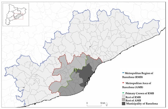
Figure 2.
Barcelona Metropolitan Region (RMB) study area: EMEF transportation analysis zones (TAZ-EMEF). The Municipality of Barcelona is divided into 10 districts (not shown).
The area is covered by the TAZ-EMO zoning system (582 transportation zones) for transportation planning purposes. The travel survey’s zoning system is TAZ-EMEF (see Table 2) and each TAZ-EMEF zone contains several aggregated TAZ-EMO zones.
Table 2.
Number of zones in the TAZ-EMEF zoning system.
2.3. Datasets
In this study, we used four consecutive surveys of the Barcelona Metropolitan Region (RMB), the Working Day Mobility Survey (EMEF) [36] from 2018 to 2021 [37]. It includes individual characteristics and a list of trips made the day before. The sample design for the EMEF travel survey guarantees representativeness of the population. The technical team responsible for the sample design on behalf of the authorities assured its quality.
Additionally, along with the trip purpose and travel mode required to build up the daily activity sequence data, we included the following relevant individual information from the surveys:
- Education: A qualitative variable that divides education into basic, secondary, and higher education levels;
- Professional activity: Retired, unemployed, homemaker, student, or active;
- Gender: Male or female;
- Age groups: 16–29, 30–44, 45–64, and 65 and above;
- Other factors included car availability, residential area, mode use frequency, etc.
2.4. Data Processing
The following points summarize the study’s processes and decisions:
- Data orchestration was needed to account for the 4 EMEF sources because they were delivered independently and the recorded fields differed. The orchestration of EMEF datasets involves selecting common subsets of fields and reordering them appropriately. While EMEF data allow access to specific periods of the day, data orchestration addresses the total number of daily trips;
- The characteristics of trip-makers in EMEF datasets are gender (2 categories) and age (16–29, 30–44, 45–64, and 65 and above). EMEF 2019, 2020, and 2021 datasets do not contain a residential zone for each unit (trip-maker) but it was imputed using the origin zone for the first trip of the day in home-based trips. This means that some units lack a TAZ-EMEF residential area (only residential county is known); this subsample is less than 5% of the sample size;
- EMEF datasets contain the characteristics education level (none, primary, secondary, or higher) and professional status (student, active, unemployed, retired, or non-active). Unfortunately, family size and structure are missing on 3 out of 4 EMEF travel surveys. These were included in the survey after 2021, so they will be analyzed in the near future;
- The maximum number of modes collected for any trip is 3. The travel time for each trip segment is unavailable; just the overall trip travel time is available (in minutes);
- Individual sample sizes in RMB are 9930, 9934, 10,024, and 10,028 for 2018 to 2021, respectively, and the total number of trips in the sample is 39,318, 40,276, 34,714, and 35,209, respectively. After filtering professional drivers and inconsistent data, the total sample size for individuals is 37,877 units. Travel surveys are cross-sectional; no panels are available;
- A total of 11 activities and travel modes were considered: escorting (A), occasional activity (C), staying at home (H), going to school/university (S), recurrent daily activities such as shopping, visiting family (O), and working (W) and the travel modes were walking (TW), cycling (TB), public transport (TP), private vehicle (TC), and e-scooter or Segway (TM).
3. Methodological Approach
The proposed methodology derives activity sequences from travel diaries and analyzes travel behavior patterns. Most travel surveys collect information about individuals (socioeconomic, demographic, etc.), their household (size, structure, relationships), their transportation habits, and travel diaries (start and end location, start and end time, travel mode, purpose of travel, etc.) on a given day, usually a workday.
Applying this approach to travel surveys and daily travel behavior involves the following steps:
- Data preprocessing: The data need to be preprocessed before applying SA. This involves cleaning the data, handling missing values and multivariate outliers, and organizing the data into sequences based on the order of activities [38]. Each individual’s sequence of activities becomes a series of ordered events. Quantitative time-fragmentation indicators are elaborated;
- Sequence mining: Data analytics algorithms are applied to identify common patterns and sequences found within the dataset after the data processing step. These algorithms can reveal frequent sequences, such as common travel patterns or recurring combinations of activities [32,39,40]. Activity sequences are qualitative time series; proposals have been made in the literature to quantify the degree of similarity between sequences. We selected a data analytics approach and considered similarities after projecting activity sequences in a real space resulting from multiple correspondence analysis (MCA) [41]. Euclidean distances were applied to assess the similarities between projected sequences;
- Travel behavior comparison: SA allows comparisons of sequences between individuals or groups [32,39,40]. By comparing sequences, researchers can identify typical or representative travel behavior patterns that can help in understanding variations in travel behavior based on demographic characteristics, such as age, gender, or socioeconomic status;
- Clustering and typology: Clustering of projected activity sequences obtained by MCA [41] identifies distinct groups or clusters of individuals based on travel behavior patterns. After clustering individuals with similar projected sequences, we can identify typologies or travel behavior profiles representing different population segments.
A statistical analysis of sequences and fragmentation indicators allows a greater depth of analysis, as indicated by the workflow shown in Figure 3 (the methodological workflow is inspired by [16]). Some potential lines of analysis rely on developing a general linear model using a fragmentation indicator as a target variable and quantitative and qualitative explanatory variables such as gender, education, day principal mode, etc. The marginal effects of explanatory variables help to clarify the multivariate association with the characteristics of individual units.
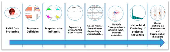
Figure 3.
Methodological workflow. From EMEF datasets, sequences in a day are defined in minutes. Once fragmentation variables are calculated, exploratory analysis is carried out and linear models are developed for each one based on the socioeconomic characteristics of sample units. Once the basic statistical analysis is completed and multivariate data reduction is applied, daily sequences are classified to identify segments of travel pattern behaviors.
The sequences for all sampled units in the EMEF 2018 to 2021 travel surveys weighted by its expansion factor were produced by using the TraMineR package in RStudio [32,42]. Afterward, fragmentation indicators (entropy, turbulence, complexity, and TTR) were elaborated from daily travel sequences using functions in the TraMineR package of RStudio.
The principal transport mode for trips and daily primary mode labeling were determined based on PCA and unsupervised classification [41].
3.1. Descriptive Analysis
Firstly, we conducted a basic descriptive analysis of fragmentation indicators for activity sequences of sample units in 2018 to 2021 EMEF travel surveys, including the following:
- Distribution of fragmentation variables for trip-makers and non-trip-makers;
- Univariate and multivariate outlier detection based on the robust Mahalanobis distance [43];
- Spearman correlation coefficient between fragmentation variables with/without multivariate outliers to assess the association between selected fragmentation variables.
3.2. Data Dimension Reduction
We applied a data reduction technique to the dataset of daily sequences such that the number of columns (number of minutes by number of activities, in this case 11) retained represented the first N = 500 factorial axes in the multiple correspondence analysis (MCA) using the FactoMineR package in R [44,45], which accounted for more than 90% of data variability from 6 to 24 h. Our input matrix for MCA was a 37,877 × 11,880 matrix (complete disjunctive encoding) containing activities from the selected list (11 options), where each column represents one category of the minute factor (11 possible levels accounting for activities plus transportation options) and the output was a 37,877 × 500 matrix.
This procedure is effective for handling such a large dataset, which in our case comprised daily sequences. Our database thus remained highly detailed, as we maintained relevant information based on 1 min rather than aggregating the timeframes, which would lead to information loss. Recording activities for each 1 min of the day is the most suitable method to maintain the level of detail.
Multiple correspondence analysis projection ensures the utilization of all available information (minute-to-minute activities) and avoids distortions during dimensionality reduction. The reduction is based on the extended Kaiser criteria [46], with the retained factorial axes accounting for more than 90% of data variability, thus ensuring representativeness. These factorial axes were used to project the sequences into the new space, which achieved 95% dimension reduction and allowed the possibility of handling non-supervised clustering based on real numbers (instead of qualitative variables with 11 categories).
Then, we projected the data sequences in the N-dimension factorial space. Sequence projections are vectors of N real numbers. We applied hierarchical clustering to discover data clusters showing similar daily sequences. The clusters were profiled based on characteristics and numerical variables from 2018 to 2021.
For clustering analysis, the similarity/dissimilarity matrix had millions of cells (37,877 × 37,877) containing the dissimilarity scores for the sequences of every person in the working sample. Using seqdist() in the TraMineR package in R allowed us to calculate the dissimilarity matrix based on several metrics [31] of the original minute sequences. However, it was not feasible in the original space due to large memory requirements. For this reason, we performed multiple correspondence analysis (MCA) for data reduction instead of principal component analysis (PCA, suitable for numeric variables) to detect the underlying structures in the dataset before clustering.
After data reduction was performed on all activity sequences (including multivariate outliers), we used clustering to group sequences of activities with similar dissimilarity scores obtained from the sequence comparison after projection. The fragmentation indicators and characterization variables of sample units helped in interpreting the clusters. We determined the final number of clusters by using an optimized criterion for balancing within-group similarity and between-group dissimilarity. Specifically, we applied hierarchical clustering (HC) [41] to the reduced projected data of daily travel patterns in the minute activity matrix. Each cluster comprised points that were more similar than those in other groups. The hierarchical clustering method in the FactoMineR package can reduce the computational burden by starting the agglomerative process on a heuristic partition that represents 10% of the original length. We cut the hierarchical agglomerative tree at a degree of similarity of almost 40%, using a balanced combination of common techniques such as the between sum of squares to the total sum of squares, the gap statistic, and the silhouette method.
3.3. Defining the Principal Travel Mode
In metropolitan areas, trips can be composed of several modes: someone can leave home in a car as a passenger to get to a bus stop and, at some point, transfer to the train and arrive at the destination after a 5 min walk. The concept of principal mode is tricky and usually involves some decision making. The maximum number of user modes is a design parameter in survey K; sometimes, the travel time spent in each stage is unknown. Let us assume that the sequence of modes used in a trip is mode1, …, modeK.
Rules of assigning principal trip mode (gmode) for K = 3:
- If mode1 is defined and mode2 is none, then the principal mode (gmode) is code1;
- If mode1 and mode2 are defined and mode3 is none, then gmode is code1:code2. For example, if mode1 is driving a car and mode2 is riding the bus, then gmode becomes C:B;
- If mode1, mode2, and mode3 are defined, then gmode is code1:code2:code3. For example, if mode1 is driving a car, mode2 is riding the train, and mode3 is riding the bus, then gmode becomes C:T:B;
- Repeat the process until the maximum number of stages has been considered;
- If data preparation shows some drawbacks, such as mode1 and mode3 are none and mode2 is defined, then gmode is defined as code2;
- If mode2 and mode3 are defined and mode1 is none, then gmode is code2:code3.
If the trip segment duration is known, then the principal mode assignment can be based on the mode that takes the longest time. Otherwise, it can be applied after a preprocessing step:
- Identify gmode frequencies once the number of possibilities is reduced based on unordered sets. For example, using a car and a bus would be indicated as C:B and assimilated to B:C (alphabetical order of the set code modes). Any mode composition involving W (walking) is also set to non-walking mode. For example, T:W is designated as T (train);
- The number of occurrences of each code for each trip survey is considered and principal component analysis is applied to the data matrix composed of n rows (as many as the total number of trips in the sample) and as many columns as mode codes. Unsupervised clustering analysis after principal component analysis defines the final number of clusters, which are groups of transportation modes used during individual trips. Thus, representative modal cluster combinations set the principal travel mode.
Each individual’s principal modes during a workday help in labeling modal preferences for the expanded population. The same steps can be followed to define day principal mode (dpmode), considering all daily trips.
3.4. Fragmentation Variable Profiling
Each fragmentation variable determined a significant global association with quantitative and qualitative variables that characterize sample units, in this case, individuals. The quantitative variables are the number of daily trips and the total travel time in a day and the qualitative variables are gender, education, profession, principal daily mode, declared modal preferences, etc. Each fragmentation variable quantifies the quantitative variables related to sample units, qualitative variables where the mean value of the fragmentation indicator is not homogenous for all categories, and categories where the mean value of the indicator is significantly different from the overall mean at 99% confidence.
We then used Tukey’s multiple comparisons test of means at 95% confidence, a particular case of the multiple comparison test (MCT). Tukey’s honestly significant difference (HSD) test can be used under the assumption of equal variance. Tukey’s test is considered a reliable method of detecting differences during pairwise comparison (it is less conservative than others when applied to small samples) and can increase the probability of rejecting the null hypothesis when there is a small group size (this was not a problem in our dataset since we needed to make comparisons by year and the sizes were large enough to justify the theoretical assumptions). Tukey’s HSD implemented in R [47] is the Tukey–Kramer test (a modification of the original HSD to cope with unbalanced data).
4. Results
This section presents the results of the analyses conducted in this study.
4.1. Descriptive Analysis
This section presents the descriptive analysis of fragmentation indicators between 2018 and 2021. We derived fragmentation indicators from daily travel sequences using functions in the TraMineR package of RStudio [39]. Table 3 shows fragmentation indicators calculated for the daily sequences shown in Table 1. Figure 4 graphically depicts the exploratory analysis of fragmentation indicators. At the top of Figure 4, bivariate plots include the whole sample of trip-makers; at the bottom, histograms for the same variables exclude multivariate outliers at a 99% confidence level based on the robust Mahalanobis distance [43]. Non-parametric Spearman correlation coefficients between fragmentation indicators excluding multivariate outliers show a direct association, with more intensity noted for the complexity–turbulence pair: 0.6 (entropy–turbulence), 0.91 (complexity–turbulence), and 0.85 (complexity–entropy).
Table 3.
Examples of daily travel patterns for three units of working sample based on 11 activities.
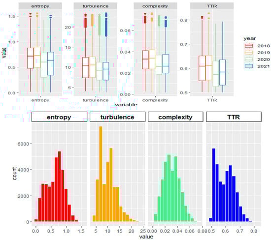
Figure 4.
Fragmentation indicators. Top: bivariate plots for all trip-makers; middle: boxplots by year; bottom: histograms excluding multivariate outliers (99% confidence).
The entropy indicator has the maximum value when all possible activities appear in a sequence and the total duration for each activity is the same. In a sequence where staying home takes up all the daily minutes, entropy is 0 (minimum), and the maximum for 11 activities is 2.40. The fragmentation of daily time into many episodes weighted by duration is accounted for by turbulence, i.e., many shorter episodes mean more stress when handling all duties. In contrast, complexity considers the number of transitions between episodes, the number of activities represented, and their total duration. Stress in daily life is captured mainly by turbulence since transitions between activities use at least one transport mode. In comparison, complexity combines entropy and turbulence characteristics.
To understand the meaning of the fragmentation indicators, we selected a subset of trip-makers in the 1%, 50%, and 99% percentile for turbulence indicators. The results are presented in Figure 5.
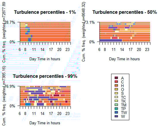
Figure 5.
Some activity sequences in the 1%, 50%, and 99% percentile groups for turbulence. Trip-makers subset and multivariate outliers are excluded.
The radar plot in Figure 6 shows the four fragmentation indicators, total trips, and total travel time in a day relative to mean values over the years. The COVID-19 effects can be seen in 2020 fragmentation variables: they have the smallest values, while those for 2018–2019 have the highest, and 2021 recovery was not as expected, revealing that some behavioral changes that may have been latent before COVID-19 and were potentiated by the pandemic seem to remain after it. This will be clarified once the data for 2022 and beyond can be analyzed.
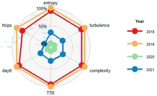
Figure 6.
Fragmentation indicators according to EMEF travel survey year. Ttrips indicates the total number of trips and daytt indicates the total time traveling in a day.
4.2. Modal Frequency and Residential Area
Travel surveys offer multiple possibilities for multivariate exploratory analysis; this section illustrates how declared modal use frequency (generic modal preferences) is connected to individual characteristics such as place of residence. These findings open a new line of research in which spatial representation is critical. The first factorial plane of multiple correspondence analysis applied to individual modal preferences and residential areas (see Figure 7) shows increasing frequency of use of public transport and rare use of cars by residents of Barcelona city (BCN). In contrast, frequent car use and non-active modes are found in the outer metropolitan region (RMB). The vertical axis has a spatial meaning (negative to positive values as external to the inner metropolitan area) and the horizontal axis has a temporal meaning (positive values are associated with 2020–2021, clearly separate from the negative values for 2018–2019).
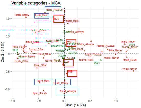
Figure 7.
First factorial plane: modal preferences and residential areas across years. Residential areas are highlighted in the red box and modal preferences correspond to those in the blue box. fcard, car as driver; fcarnd, car as non-driver; fwalk, walking; ftpub, public transport; fbike, bike; fmicro, e-scooter/Segway. BCN, Barcelona city; EMT, Primary Crown; AMB, Barcelona Metropolitan Area; RMB, Metropolitan Region of Barcelona. Year, gender, age group, and activity are shown in green.
4.3. Linear Models for Fragmentation Indicators
One line of analysis that considers variables that affect fragmentation indicators is linear modeling. For example, in the case of the complexity indicator, linear model results show a significant dependency (marginal effect once all other significant variables are included) on year, the interaction of gender and age group, activity, residential area, and education.
Figure 8 shows the marginal effects of gender by age group across years on the complexity indicator. There is significantly greater complexity for women in the 30–44 year age group than men (all years except 2020), while the opposite is clearly seen for women 65 and older (any year). A second analysis involving the travel time ratio (TTR) indicator as the target variable in a linear model showed a pattern when comparing 2018–2019 against 2020–2021 data, where TTR in 2021 did not seem to return to values before COVID-19. Education is an important factor; those with a higher level of education spent more of their daily time away from home before COVID-19 than those with other levels of education (none, primary, and secondary), in contrast to 2021 (see Figure 9). More highly educated people spent increased time at home during 2020 and 2021; teleworking had a remarkable impact on this group after COVID-19, and differences across residential areas have been minimized, according to 2021 data. The higher-educated group had a more remarkable increase in home-stay time from 2019 to 2020 than the other education groups, for whom telework was not an option.
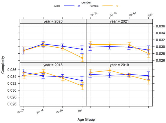
Figure 8.
Marginal effects of age group on complexity indicator by gender across years.
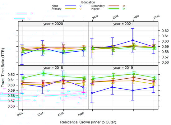
Figure 9.
Marginal effects of a residential area on TTR by education across years.
4.4. Principal Mode
As noted in Section 3, one step in data processing relies on defining the day principal mode (dpmode). We elaborated this variable according to the frequency of transportation modes recorded in the transitions between activities in the sample (2018 to 2021) and unsupervised classification. The first factorial axis separates the day principal modes of private transport (negative values) and public transport (positive values) and the second factorial axis splits the sample into more pedestrians (negative values) and fewer pedestrians (positive values) (see Figure 10).
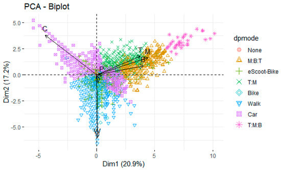
Figure 10.
Day principal mode clusters based on the number of activity occurrences in daily trips. Multimodal labels M:B:T, combined metro plus bus and train last mode; T:M:B, combined train first, metro plus bus modes; T:M bimodal train and metro.
4.5. Clustering
The five largest clusters exhibit distinct distributions of entropy, turbulence, complexity, and travel time ratio, highlighting the divergent behaviors of individuals within each cluster regarding these indicators (see Figure 11). These clusters account for 37% of the sample variability, with a median size of 145 units; 90% comprise fewer than 800 units and 90% contain more than 10 units. The largest cluster consists of non-trip-makers (4190 units), with a value of 0 for entropy, turbulence, and complexity. TTR is 0.5 (this cluster does not appear in the sequence state analysis shown in Figure 12). The hierarchical clustering method was employed after dimensionality reduction through multiple correspondence analysis factorial projections of sequences according to standard multivariate data reduction techniques, as explained in Section 4.2, since this mitigates biases resulting from information loss.
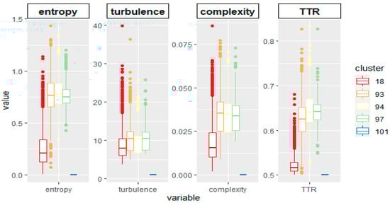
Figure 11.
Fragmentation indicators in five largest clusters after activity sequence classification.
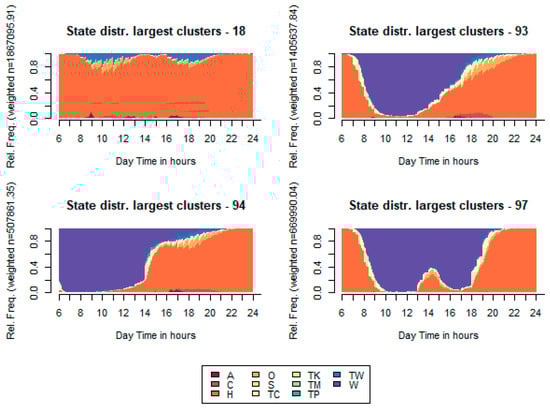
Figure 12.
State distribution of the four largest clusters after activity sequence classification.
Clusters 93, 94, and 97 show people mainly involved in work activities but the patterns are not the same. Cluster 94 includes people whose shifts start very early in the morning and who conduct after-work activities, while people in clusters 93 and 97 start their work activity later in the morning, and 97 includes people who take a break during their shift to eat lunch at home, not in the workplace as those in cluster 93 do. Cluster profiling reveals additional characteristics of these units.
Although we do not include profiling details in this paper, the following is a summary of these findings:
- Cluster 18: Retired, primary education or handicapped, over 65 years, origin is the rest of Spain;
- Cluster 93: High education level, professionally active, 30–44 years of age, origin is Catalonia, private car use score 13 points over the overall mean;
- Cluster 94: Primary or secondary education, professionally active, 30–64 years of age, foreign origin, private transport use score 15 points over the overall mean;
- Cluster 97: High education level, professionally active, 30–64 years of age, origin is Catalonia, private car use score 26 points over the overall mean.
A more in-depth analysis of clusters overrepresented by males and females shows remarkable differences between activity sequences (see Figure 13). In clusters containing more than 65% males, early morning and afternoon shifts (clusters 94 and 83) and extended shifts (cluster 100) with occasional escorting activities are seen. In clusters containing more females, escorting is prevalent, especially in the after-school period (usually after work) in clusters 48 and 69; in cluster 90, public transport commuter mode for travel to the workplace is seen. Profiling details are not included in this paper. However, the main findings can be summarized as follows:
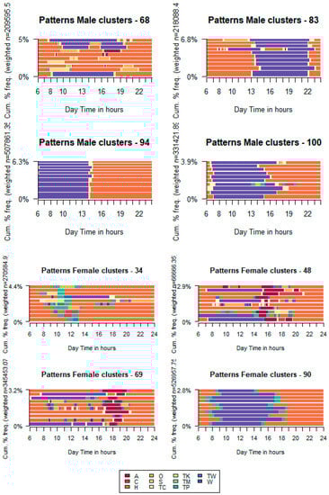
Figure 13.
Daily sequence activity according to clusters overrepresented by males and females.
- Cluster 68: E-scooter users, unemployed or students, Barcelona city residents;
- Cluster 83: Age 16–29, secondary education, active, car users, RMB residents;
- Cluster 94: Primary education, professionally active, origin is Catalonia, engaged in non-flexible job schedule and public transport use, mostly Primary Crown or AMB residents;
- Cluster 100: High education level, professionally active, flexible work schedule, private car use score 26 points over the overall mean, RMB residents;
- Cluster 34: Retired, over the age of 65, or unemployed young people or students living in Barcelona city;
- Cluster 48: Primary education, unemployed, mostly escorting activity using a car in RMB area;
- Cluster 69: Age 30–44, homemakers, mostly escorting activity using a car, resident of RMB or AMB area;
- Cluster 90: Higher education level, non-flexible work schedule, public transport users, residents of Barcelona city. Foreign origin is overrepresented.
Fragmentation indicators are helpful to complement the previous interpretation (Figure 14). We can see the mean values of fragmentation indicators on radar plots for selected clusters with either male or female overrepresentation. Cluster 68, which is predominantly male, contains patterns involving considerable turbulence and complexity, without remarkable entropy or TTR, in contrast to the predominantly male clusters 83, 94, and 100. In the case of predominantly female clusters, cluster 34 shows shallow fragmentation indicators compared to clusters 48, 69, and 90.
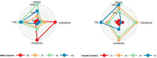
Figure 14.
Fragmentation indicators for eight clusters overrepresented by males or females.
5. Discussion
SA is a statistical method used to analyze and interpret patterns in sequential categorical time series data. When applied to travel surveys and daily travel behavior, SA can help researchers understand the sequential order and dynamics of activities undertaken during travel and their interconnections. It allows for a detailed examination of the sequences of activities individuals engage in, such as commuting, working, enjoying leisure time, and other daily routines, while also considering the number of activities, order of activities in a day, and duration. Studying daily activity sequences (including each activity and each trip) is preferable to using other techniques to study activity–travel behavior because sequences include the entire trajectory of a person’s activity during the day, as indicated by some authors [5]. Comparing our findings to those in [5], we used all sample units during four EMEF surveys and the whole study area instead of restricting the analysis to a subarea. Compared to [25], 15 activities were considered activities. Still, transport was regarded as a single activity (transition between activity states), while in our research, transportation modes were explicitly considered in the transitions between activity states. Our approach highlights the importance of multimodality in European metropolitan areas.
Some authors [48] found that the duration of free time and personal business activities were very similar between men and women. In contrast, women spent significantly more time shopping. If we extend this result, activity sequences in clusters overrepresented by women show remarkable differences from those dominated by men.
In our case, the lack of family size and structure data in the collected 2018 to 2020 EMEF data was a limitation with regard to enhancing linear models for fragmentation indicators and classification profiling. We expect to extend our analysis once EMEF data from 2021 and beyond are available since these data seem to play an essential role according to the literature [49].
The impact of telework has been addressed by some authors, such as Bayarma et al. [50]. This feature was not collected in the EMEF travel survey until 2020 and is a limitation in the current paper. Analyzing activity sequences and fragmentation indicators according to telework availability is a promising research topic because telework is linked to both education level and type of job. Medical staff, essential educators, and service staff have limited teleworking opportunities. In addition, the previously cited positions are mainly filled by women.
Understanding the daily activity and travel patterns of transit users is fundamental for transportation authorities in European cities. Hence, classifying transit-based activity sequences is an important topic in order to improve transit performance and in turn the sustainability of metropolitan areas [51].
6. Conclusions
SA was applied to EMEF travel surveys and various data analytics techniques were used to analyze daily travel behavior according to the following steps:
- Data preprocessing: Each individual’s sequence of activities becomes a series of ordered events. Entropy, turbulence, complexity, and travel time ratio (TTR) indicators were elaborated using the TraMineR method in RStudio. Regarding fragmentation variables, 1190 out of 37,877 units were multivariate outliers (3%); they were not discounted but were used as supplementary observations when applying data analytics;
- Sequence mining: Data analytics algorithms were applied to identify the profiles of fragmentation indicators within the EMEF dataset. Data reduction based on MCA allows activity sequences defined at the minute level to be projected into a multivariate real space, reducing the computational burden. Euclidean distances were applied to assess the similarities between projected sequences. This is an innovative feature of our research;
- Sequence comparison: Based on fragmentation indicators as target variables, linear models were used to highlight variations in travel behavior based on demographic characteristics such as age, gender, and socioeconomic status;
- Clustering and typology: Clustering of projected activity sequences identified distinct segments or clusters of individuals based on their travel behavior patterns. We obtained 10% of the clusters over 800 sample units. After clustering individuals with similar projected sequences, we developed typologies or travel behavior profiles, focusing on clusters over- and underrepresented by males and females. The clustering process considered all activity sequences, leading to many small clusters grouping multivariate outliers. We also paid attention to the four largest clusters.
Large cluster typologies can inform transportation planners and stakeholders about policy making, allowing them to focus on targeted interventions by segment. In the case study, 10 clusters grouped more than 50% of activity sequences. A lack of mobility affected 11% of the population.
Modal use frequency and residential area parameters have a remarkable association that will be addressed in future research. The built environment also seems to play a critical role.
The characterization of activity sequences will be refined as soon as household composition and teleworking data are available and new yearly travel surveys are processed (from 2021). Our agreement with ATM will give us access to 2022 data when they become available, hopefully before 2024. Then, in the forthcoming work, we will check whether the conjecture about the behavioral changes is correct.
Author Contributions
Conceptualization, L.M., L.M.-D. and J.B.; formal analysis, L.M., L.M.-D. and J.B.; funding acquisition, L.M. and J.B.; methodology, L.M., L.M.-D. and J.B.; software, L.M.; supervision, J.B.; writing—original draft, L.M.; writing—review and editing, L.M.-D. and J.B. All authors have read and agreed to the published version of the manuscript.
Funding
This research was funded by Spanish R+D Programs (PID2020-112967GB-C31) and by Secretaria d’Universitats-i-Recerca-Generalitat de Catalunya—2021 SGR 01252 Information Modeling and Processing.
Data Availability Statement
Restrictions apply to the availability of EMEF data. Anonymized data were obtained from the Autoritat del Transport Metropolità (ATM) and datasets cannot be distributed without their permission.
Acknowledgments
EMEF datasets, previously processed, were kindly shared by the Autoritat del Transport Metropolità (ATM). Their contribution to our research is gratefully acknowledged
Conflicts of Interest
The authors declare no conflict of interest.
References
- Rodrigue, J.-P.; Comtois, C.; Slack, B. The Geography of Transport Systems, 4th ed.; Routledge: New York, NY, USA, 2017; ISBN 978-1-317-21010-8. [Google Scholar]
- Mejía-Dorantes, L.; Montero, L.; Barceló, J. Mobility Trends before and after the Pandemic Outbreak: Analyzing the Metropolitan Area of Barcelona through the Lens of Equality and Sustainability. Sustainability 2021, 13, 7908. [Google Scholar] [CrossRef]
- Lyons, G.; Mokhtarian, P.; Dijst, M.; Böcker, L. The dynamics of urban metabolism in the face of digitalization and changing lifestyles: Understanding and influencing our cities. Resour. Conserv. Recycl. 2018, 132, 246–257. [Google Scholar] [CrossRef]
- Mejía-Dorantes, L.; Soto Villagrán, P. A review on the influence of barriers on gender equality to access the city: A synthesis approach of Mexico City and its Metropolitan Area. Cities 2020, 96, 102439. [Google Scholar] [CrossRef]
- McBride, E.; Davis, A.; Goulias, K. Fragmentation in Daily Schedule of Activities using Activity Sequences. Transp. Res. Rec. 2019, 2673, 844–854. [Google Scholar] [CrossRef]
- McBride, E.C.; Davis, A.W.; Goulias, K.G. Exploration of Statewide Fragmentation of Activity and Travel and a Taxonomy of Daily Time Use Patterns using Sequence Analysis in California. Transp. Res. Rec. 2020, 2674, 38–51. [Google Scholar] [CrossRef]
- Nobis, C.; Lenz, B. Gender Differences in Travel Patterns: Role of Employment Status and Household Structure. In Proceedings of the Research on Women’s Issues in Transportation, Chicago, IL, USA, 18–20 November 2004; TRB Publications Office 1073-1652; pp. 114–123. [Google Scholar]
- Baratian-Ghorghi, F.; Zhou, H. Investigating Women’s and Men’s Propensity to Use Traffic Information in a Developing Country. Transp. Dev. Econ. 2015, 1, 11–19. [Google Scholar] [CrossRef]
- Stopher, P.; Stecher, C. (Eds.) Travel Survey Methods; Emerald Group Publishing Limited: Bingley, UK, 2006; ISBN 978-0-08-044662-2. [Google Scholar]
- Stopher, P.R.; Wilmot, C.G.; Stecher, C.; Alsnih, R. Household Travel Surveys: Proposed Standards and Guidelines. In Travel Survey Methods; Stopher, P., Stecher, C., Eds.; Emerald Group Publishing Limited: Bingley, UK, 2006; pp. 19–74. [Google Scholar]
- Stopher, P.R.; Greaves, S.P. Household travel surveys: Where are we going? Transp. Res. A 2007, 41, 367–381. [Google Scholar] [CrossRef]
- Van Evert, H.; Brög, W.; Erl, E. Survey Design: The Past, the Present and the Future. In Travel Survey Methods; Stopher, P., Stecher, C., Eds.; Emerald Group Publishing Limited: Bingley, UK, 2006; pp. 75–93. [Google Scholar]
- Cambridge Systematics; Travel Model Improvement Program (U.S.); Environmental Protection Agency. Travel Survey Manual. 1996. Available online: https://rosap.ntl.bts.gov/view/dot/13222 (accessed on 8 September 2023).
- Stopher, P.R. Use of an activity-based diary to collect household travel data. Transportation 1992, 19, 159–176. [Google Scholar] [CrossRef]
- Goldenberg, L. Choosing a Household Survey Method: Results of Dallas—Fort Worth Pretest. Transp. Res. Rec. 1998, 1625, 86–94. [Google Scholar] [CrossRef]
- Montero, L.; Mejía-Dorantes, L.; Barceló, J. The role of life course and gender in mobility patterns: A spatiotemporal sequence analysis in Barcelona (In review). Eur. Transp. Res. Rev. 2023; in review. [Google Scholar]
- Bhat, C.R.; Goulias, K.G.; Pendyala, R.M.; Paleti, R.; Sidharthan, R.; Schmitt, L.; Hu, H.-H. A Household-Level Activity Pattern Generation Model with an Application for Southern California. Transportation 2013, 40, 1063–1086. [Google Scholar] [CrossRef]
- Bhat, C.R. A generalized multiple durations proportional hazard model with an application to activity behavior during the evening work-to-home commute. Transp. Res. Part B Methodol. 1996, 30, 465–480. [Google Scholar] [CrossRef]
- Bhat, C.R. A hazard-based duration model of shopping activity with nonparametric baseline specification and nonparametric control for unobserved heterogeneity. Transp. Res. Part B Methodol. 1996, 30, 189–207. [Google Scholar] [CrossRef]
- Ettema, D.F.; Borgers, A.W.J.; Timmermans, H.J.P. Competing risk hazard model of activity choice, timing, sequencing, and duration. Transp. Res. Rec. 1995, 1493, 101–109. [Google Scholar]
- Kitamura, R.; Chen, C.; Pendyala, R.M. Generation of Synthetic Daily Activity-Travel Patterns. Transp. Res. Rec. 1997, 1607, 154–162. [Google Scholar] [CrossRef]
- Axhausen, K.; Zimmermann, A.; Schönfelder, S.; Rindsfüser, G.; Haupt, T. Observing the rhythms of daily life: A six-week travel diary. Transportation 2002, 29, 95–124. [Google Scholar] [CrossRef]
- Miller, E.J.; Roorda, M.J. Prototype Model of Household Activity-Travel Scheduling. Transp. Res. Rec. 2003, 1831, 114–121. [Google Scholar] [CrossRef]
- Goulias, K.G.; Bhat, C.R.; Pendyala, R.M.; Chen, Y.; Paleti, R.; Konduri, K.C.; Huang, G.; Hu, H.H. Simulator of activities, greenhouse emissions, networks, and travel (SimAGENT) in Southern California: Design, implementation, preliminary findings, and integration plans. In Proceedings of the 2011 IEEE Forum on Integrated and Sustainable Transportation Systems, Vienna, Austria, 29 June–1 July 2011; pp. 164–169. [Google Scholar] [CrossRef]
- Su, R.; McBride, E.C.; Goulias, K.G. Pattern recognition of daily activity patterns using human mobility motifs and sequence analysis. Transp. Res. Part C Emerg. Technol. 2020, 120, 102796. [Google Scholar] [CrossRef]
- Abbott, A. Sequences of Social Events: Concepts and Methods for the Analysis of Order in Social Processes. Hist. Methods A J. Quant. Interdiscip. Hist. 1983, 16, 129–147. [Google Scholar] [CrossRef]
- Abbott, A.; Forrest, J. Optimal Matching Methods for Historical Sequences. J. Interdiscip. Hist. 1986, 16, 471. [Google Scholar] [CrossRef]
- Abbott, A.; Tsay, A. Sequence Analysis and Optimal Matching Methods in Sociology: Review and Prospect. Sociol. Methods Res. 2000, 29, 3–33. [Google Scholar] [CrossRef]
- Abbott, A.; DeViney, S. The Welfare State as Transnational Event: Evidence from Sequences of Policy Adoption. Soc. Sci. Hist. 1992, 16, 245. [Google Scholar] [CrossRef]
- Leszczyc, P.T.L.P.; Timmermans, H. Unconditional and conditional competing risk models of activity duration and activity sequencing decisions: An empirical comparison. J. Geogr. Syst. 2002, 4, 157–170. [Google Scholar] [CrossRef]
- Studer, M.; Ritschard, G. What matters in differences between life trajectories: A comparative review of sequence dissimilarity measures on JSTOR. J. R. Stat. Soc. A 2016, 179, 481–511. [Google Scholar] [CrossRef]
- Gabadinho, A.; Ritschard, G.; Müller, N.S.; Studer, M. Analyzing and Visualizing State Sequences in R with TraMineR. J. Stat. Softw. 2011, 40, 1–37. [Google Scholar] [CrossRef]
- Elzinga, C.H.; Liefbroer, A.C. De-standardization of family-life trajectories of young adults: A cross-national comparison using sequence analysis. Eur. J. Popul. 2007, 23, 225–250. [Google Scholar] [CrossRef]
- Ritschard, G. Measuring the Nature of Individual Sequences. Sociol. Methods Res. 2021, 1–34. [Google Scholar] [CrossRef]
- Dijst, M.; Vidakovic, V. Travel time ratio: The key factor of spatial reach. Transportation 2000, 27, 179–199. [Google Scholar] [CrossRef]
- Institut-Metropoli Working Day Mobility Surveys (EMEF)—Mobility Observatory in Catalonia (OMC)—ATM. Available online: https://omc.cat/en/w/surveys-emef (accessed on 8 September 2023).
- Institut-Metropoli Barcelona Metropolitan Area Weekday Mobility Survey (EMEF). Available online: https://www.institutmetropoli.cat/ca/enquestes/enquestes-de-mobilitat/#1447843451840-2-0 (accessed on 15 May 2023).
- Gibert, K.; Sànchez-Marrè, M.; Izquierdo, J. A survey on pre-processing techniques: Relevant issues in the context of environmental data mining. AI Commun. 2016, 29, 627–663. [Google Scholar] [CrossRef]
- Gabadinho, A.; Ritschard, G.; Studer, M.; Muller, N.S. Mining Sequence Data in R with the TraMineR Package: A User’s Guide; University of Geneva: Geneva, Switzerland, 2011; p. 129. [Google Scholar]
- Gabadinho, A.; Ritschard, G.; Studer, M.; Müller, N. Indice de complexité pour le tri et la comparaison de séquences catégorielles—Editions RNTI. In Proceedings of the Extraction et Gestion des Connaissances (EGC’2010), Hammamet, Tunisia, 26–29 January 2010; pp. 61–66. [Google Scholar]
- Husson, F.; Lê, S.; Pages, J. Exploratory Multivariate Analysis by Example Using R Analysis; Chapman & Hall: London, UK, 2010; ISBN 9781138196346. [Google Scholar]
- RStudio-Team. RStudio: Integrated Development for R; RStudio Team: Boston, MA, USA, 2022. [Google Scholar]
- Mahalanobis, P.C. On the generalised distance in statistics. Proc. Natl. Inst. Sci. India 1936, 2, 49–55. [Google Scholar]
- Lê, S.; Josse, J.; Husson, F. FactoMineR: An R Package for Multivariate Analysis. J. Stat. Softw. 2008, 25, 1–18. [Google Scholar] [CrossRef]
- R Core Team. R: A Language and Environment for Statistical Computing; R Foundation for Statistical Computing: Vienna, Austria, 2021. [Google Scholar]
- Kaiser, H.F. The application of electronic computers to factor analysis. Educ. Psychol. Meas. 1960, 20, 141–151. [Google Scholar] [CrossRef]
- Tukey, J.W.; Brillinger, D.R.; Cox, D.R.; Braun, H.I. The Collected Works of John W. Tukey; Wadsworth Advanced Books & Software: Belmont, CA, USA, 1984; ISBN 9780534033033. [Google Scholar]
- Niemeier, D.A.; Morita, J.G. Duration of trip-making activities by men and women. Transportation 1996, 23, 353–371. [Google Scholar] [CrossRef]
- Hubers, C.; Schwanen, T.; Dijst, M. ICT and Temporal Fragmentation of Activities: An Analytical Framework and Initial Empirical Findings. Tijdschr. Econ. Soc. Geogr. 2008, 99, 528–546. [Google Scholar] [CrossRef]
- Ben-Elia, E.; Alexander, B.; Hubers, C.; Ettema, D. Activity fragmentation, ICT and travel: An exploratory Path Analysis of spatiotemporal interrelationships. Transp. Res. Part A Policy Pract. 2014, 68, 56–74. [Google Scholar] [CrossRef]
- Rafiq, R.; McNally, M.G. Heterogeneity in Activity-travel Patterns of Public Transit Users: An Application of Latent Class Analysis. Transp. Res. Part A Policy Pract. 2021, 152, 1–18. [Google Scholar] [CrossRef]
Disclaimer/Publisher’s Note: The statements, opinions and data contained in all publications are solely those of the individual author(s) and contributor(s) and not of MDPI and/or the editor(s). MDPI and/or the editor(s) disclaim responsibility for any injury to people or property resulting from any ideas, methods, instructions or products referred to in the content. |
© 2023 by the authors. Licensee MDPI, Basel, Switzerland. This article is an open access article distributed under the terms and conditions of the Creative Commons Attribution (CC BY) license (https://creativecommons.org/licenses/by/4.0/).