Dynamic Modulus Prediction Validation for the AASHTOWare Pavement ME Design Implementation in Egypt

Abstract

Dynamic Modulus, E* is a crucial property of the hot mix asphalt (HMA). For the AASHTOWare Pavement ME design, E* is an essential material input. E* can be measured in the laboratory or predicted using different models based on some fundamental properties of the HMA. The NCHRP 1-37A and NCHRP 1-40D prediction models are the two main models adopted by the AASHTOWare to predict the E* based on the HMA mixture volumetrics, gradation, and binder properties. The main objective of this research was to validate these two prediction models using local HMA mixes for the purpose of the regional application of the AASHTOWare Pavement ME design in Egypt. For this purpose, the E* values of ten locally plant-produced HMA mixes were measured in the laboratory. The two E* prediction models were then used to estimate the E* values for the same materials. Consequently, the performance of both models was studied by comparing the measured values to the estimated values. The results showed that the NCHRP 1-40D prediction model can satisfactorily predict the E* of the Egyptian HMA mixes with minimal bias and high accuracy. The model yielded an adjusted coefficient of determination (R²) of 0.86 based on 480 E* measurements. On the other hand, the NCHRP 1-37A prediction accuracy was not satisfactory, with very poor accuracy (Adjusted R² = 0.18) and high bias. Afterwards, the effect of the predicted E* from the NCHRP 1-40D model on the AASHTOWare Pavement ME predicted pavement performance in terms of rutting, cracking, and roughness was further studied. Accordingly, twenty-four simulation runs for typical Egyptian design cases were conducted using, first, the laboratory measured E* values and, then, the NCHRP 1-40D predicted E* values. The results showed that the NCHRP 1-40D predictions had no significant effect on the pavement performance predicted by the AASHTOWare Pavement ME with R² of the different pavement distresses ranged from 0.980, for the AC rutting, to 0.9996 for the International Roughness Index (IRI). Hence, the NCHRP 1-40D model can be used satisfactorily to predict E* for the Egyptian HMA mixes without compromising the structural pavement design.

1. Introduction

AASHTOWare Pavement ME approach is the latest and the most innovative approach to design and analyze pavements. It basically builds upon the AASHTO mechanistic-empirical pavement design guide. AASHTOWare Pavement ME Design software is the latest generation of the pavement design software. It is a tool capable of optimizing pavement designs based on given requirements allowing the user to evaluate and fine-tune the design [1]. Hence, its regional application is needed to enhance the design of flexible pavement and properly manage the pavement maintenance cycles needs. The Mechanistic Empirical (ME) design approach introduces a new philosophy of the pavement design [2]. Pavement stresses and strains are calculated using fundamental mechanistic models (the mechanistic part), while the pavement distresses such as rutting, cracking, and roughness are determined using empirical models (the empirical part). Accordingly, the empirical part needs through calibrations for its empirical models based on the prevailing local conditions [3]. The ME design has three different hierarchical input levels: level 1 (information gathered are project specific measured values), level 2 (correlations with simple properties), and level 3 (default/typical values) [2]. Depending on the degree of importance and criticality of the roadway project, the level of input is selected. Since E* is a basic material input and since not all pavement materials’ laboratories are well equipped with the E* testing set up, many E* prediction models are introduced to facilitate its determination for levels 2 and 3. Generally, for the three input levels, the main material property of the HMA layers is the E*. It is the HMA fundamental property used for the computation of the stress–strain characteristics of the different asphalt layers at their corresponding critical locations, taking into consideration the traffic loads and the environmental conditions. For level 1 input, the E* should be laboratory measured. It was stated by many researchers [2,4,5,6] that conducting the E* test in the lab consumes time and is not always feasible due to the required costly equipment and the tedious sample preparation process. Accordingly, developing one single master curve consumes time, money, and effort. As for the two other input levels (level 2 and level 3, which are the same for E*), two predictive models are used to predict the E* from the mix and binder properties [7,8,9,10]. Both E* prediction models were developed based on a large versatile dataset. These two models are: NCHRP 1-37A (Witczak viscosity-based model) [2] and the NCHRP 1-40D (Witczak complex modulus, G*, and phase angle, δ, based model) [11]. The assessment of the two Witczak predictive models, since Witczak and his research team developed both of them, to validate their suitability to be used for local conditions, was the subject of many past research studies all over the world [11,12,13,14,15,16,17,18]. Generally, it was concluded that the models’ performance varies according to the materials’ characteristics and, hence, the E* predictive models must be evaluated for regional mixtures. These E* predictive models were mainly developed, evaluated, and calibrated for certain reginal conditions. In order to be able to confidently implement these models in other regional conditions, they need to be thoroughly evaluated then calibrated if needed. Many countries all over the world carried out this evaluation, as discussed in details in the literature review section, while others are yet to conduct this task. The main research gap addressed by this study was to evaluate the effectiveness of using those E* predictive models to predict the dynamic modulus under the Egyptian regional design conditions. The novelty of this study comes from the fact that this evaluation has not been conducted yet. Hence, this study can contribute to the dynamic modulus prediction model validation for wider varieties of materials and, consequently, for the implementation of the AASHTOWare Pavement ME under wider pavement design conditions.

Thus, in order to regionally implement the AASHTOWare Pavement ME in Egypt, the E* predictive models should be locally evaluated. To locally evaluate the performance of these models, different locally plant-produced HMA mixtures were gathered from different Egyptian road projects, under construction, to reflect the most prevailing Egyptian HMA characteristics. These locally produced mixes were investigated by determining their E* in the laboratory. The properties of the studied mixtures were then used to predict their E* using the two Witczak predictive models. The performance of the predictive models was studied by two approaches: the first approach compared the measured to the predicted E* values at a wide range of temperatures and loading frequencies. Then, the accuracy and bias in the predictions were determined in terms of different goodness-of-fit statistical parameters. The second approach used the AASHTOWare to run different design cases, pertinent to the Egyptian conditions, with both measured and predicted E* to study the effect of the predicted E* on the six performance indicators of the AASHTOWare; Fatigue Cracking (FC), Thermal Cracking (TC), Longitudinal Cracking (LC), AC Rutting (R_AC), Total Rutting (R_T), and International Roughness Index (IRI). Since E* is indeed a substantial material input, its predictive values may affect the final performance of the pavement in terms of the different pavement distresses and roughness. To the knowledge of the authors, there is very limited research studies, if any, that investigated the effect of the predicted E* values on the final performance indicators determined by the AASHTOWare Pavement ME. This inspired the authors to study the effect of the Witczak E* model predictions on the pavement performance by comparing the results of the six pavement performance indicators predicted from the measured E* values versus those predicted based on the predicted E* values, for typical regional design cases.

2. Literature Review

Since HMA is a viscoelastic material, its properties can be comprehensively characterized by measuring its E*. E* is determined in the laboratory by applying a sinusoidal (haversine) axial load at different frequencies and temperatures on cylindrical HMA samples cored and sawed from gyratory compacted samples at air voids of about 7%. For different combinations of loading frequencies and temperatures, if the input is an oscillating stress, then the output will be an oscillating strain lagging the stress by a phase angle (δ).

For linear viscoelastic materials, E*is calculated by dividing the maximum stress by the recoverable axial strain. E* master curves can then be constructed based on the laboratory measured E* values.

Measuring the E* in the laboratory is a cumbersome and a time-consuming process. Accordingly, some predictive models are developed to predict the E* values based on some mix volumetric inputs and binder properties. The NCHRP 1-37A, NCHRP 1-40D, Hirsh, and Alkhateeb are among the most commonly used E* predictive models [11,12]. The majority of the available models are simple regression-based models. However, recently, there is an increasing trend in establishing E* prediction models based on machine learning. Moussa et al. [19] used a deep learning (DL) technique to develop E* prediction tool. Then, this tool was statistically evaluated. After statistically evaluating the model using different performance indicators, the model was compared to the Witczak 1-37A, Witczak 1-40 D and Hisch prediction models. This proposed technique proved itself as a reliable E* prediction tool. Behnood and Golafshani [20] used a machine learning technique to develop E* prediction model based on 4022 asphalt mixture samples. Then, this model was tested and its results were compared to the results predicted using the most commonly used E* models. It was concluded that the developed model performed well compared to the Witczak model, Hirsch model, and Artificial Neural Network (ANN) model. Xu et al. [21] conducted a comparative study of six different Machine Learning (ML) models with the a newly developed algorithm to check the probability of replacing the empirical model for predicting E*. It was concluded that E* prediction using the six ML models was promising. Moussa and Owais [19] used the transfer learning solution using deep learning (DL) technology to predict E*. A deep convolution neural networks (DCNNs) technique was used to build the E* prediction model. Daneshver and Behnood [22] developed a random forests algorithm to predict the E* using a comprehensive dataset to overcome the issues related to overestimation or underestimation reported for the previously developed Witczak models. Then, the performance of the newly developed model was assessed and compared with that of the Witczak model. The results show that the developed model can successfully estimate the E* with better performance than the Witczak models. Huang et al. [23] hybridized the ensemble and weight optimization approaches with an artificial neural network (ANN) algorithm to develop an asphalt concrete E* prediction model. The ρ200, V_beff, binder G* (dynamic shear modulus) and binder δ (phase angle) were the variables of the developed model.

The NCHRP 1-37A and NCHRP 1-40D models are among the most commonly used E* prediction models. Both models are based on the prediction of the E* from the basic mix and binder properties. The NCHRP 1-37A is based on the binder properties, whereas the NCHRP 1-40D is based on the Superpave binder properties [11,12]. The database used for the development of the NCHRP 1-40D model is wider than the NCHRP 1-37A database, since it has been increased to include 346 different HMA mixes comprises about 7400 data points. Investigating both Witczak (NCHRP) models can serve a wide spectrum of HMA mixes either designed using the Superpave or the conventional systems.

The NCHRP 1-37A model, shown in Equation (1), is developed based on a database with the characteristics shown in Table 1 [3].

$$\begin{gathered} {\log }_{10}E*=-1.249937+0.02923 {\rho }_{200}-0.001767{\left({\rho }_{200}\right)}^2-0.002841 {\rho }_4- \\ 0.058097V_a-0.82208 \frac{V_{beff}}{V_{beff}+V_a} \frac{3.871977-0.0021{\rho }_4+0.003958{\rho }_{38}-0.000017{\left({\rho }_{38}\right)}^2+0.00547{\rho }_{34}}{1+e^{(-0.603313-0.313351\log f-0.393532\log \eta ) }} \end{gathered}$$

(1)

where

• E*: The hot mix asphalt dynamic modulus, in 10⁵ psi;
• η: The asphalt binder viscosity, in 10⁶ poise;
• f: The loading frequency, in Hz;
• V_a: The air voids, %;
• V_a: The air voids, %;
• V_a: The air voids, %;
• ρ38: The cumulative retained on the 3/8” sieve, %;
• ρ4: The cumulative retained on sieve number 4, %;
• ρ200: The percentage passing Sieve No. 200.

Table 1. Dataset of the NCHRP 1-37A Model [18].

Temperature	Ranges from 0 to 130 °F
Frequency	Ranges from 0.1 Hz to 25 Hz
Binder	9 unmodified asphalt binders 14 modified asphalt binders
Aggregate	39 different types of aggregates
Asphalt Mix	unmodified asphalt binders are used with 171 mixes modified asphalt binders are used with 34 mixes
Compaction	Samples are compacted using Gyratory and Kneading
Specimen Size	Cylindrical specimen of four times eight inches for kneading compaction And Cylindrical specimens with 2.75 × 5.5 for Gyratory compaction
Aging	No aging
Data Points	2750

Table 1. Dataset of the NCHRP 1-37A Model [18].

Temperature	Ranges from 0 to 130 °F
Frequency	Ranges from 0.1 Hz to 25 Hz
Binder	9 unmodified asphalt binders 14 modified asphalt binders
Aggregate	39 different types of aggregates
Asphalt Mix	unmodified asphalt binders are used with 171 mixes modified asphalt binders are used with 34 mixes
Compaction	Samples are compacted using Gyratory and Kneading
Specimen Size	Cylindrical specimen of four times eight inches for kneading compaction And Cylindrical specimens with 2.75 × 5.5 for Gyratory compaction
Aging	No aging
Data Points	2750

When the Superpave was introduced, the binder complex shear modulus (G*) was found to be more effectively describing the asphalt binder characteristics. Accordingly, Witczak and his associates presented the revised NCHRP 1-40D model, in which both G* (asphalt complex modulus) and δ (the phase angle) were used to replace the traditional viscosity of the binder [11]. The NCHRP 1-40D model is shown in Equation (2) [11]. It is worth mentioning that both models have the same mathematical structure of a sigmoidal function.

$$\begin{array}{c}{\log }_{10}E*=0.02+0.758\hspace{0.17em}\hspace{0.17em}\left(|G_b*{|}^{-0.0009}\right)\hspace{0.17em}\times \hspace{0.33em} \left(\begin{array}{c}6.8232-0.03274{\rho }_{200}+0.00431{\rho }_{200}{}^2+0.0104{\rho }_4-0.00012{\rho }_4{}^2\\ +0.00678{\rho }_{38}-0.00016{\rho }_{38}{}^2-0.0796\hspace{0.17em}{V}_a-1.1689\hspace{0.33em}\left(\frac{V_{beff}}{V_a+V_{beff}}\right)\end{array}\right)\\ \hspace{1em}\hspace{1em}\hspace{1em}\hspace{1em}+\frac{1.437+0.03313\hspace{0.17em}{V}_a+0.6926\hspace{0.33em}\left(\frac{V_{beff}}{V_a+V_{beff}}\right)+0.00891\hspace{0.17em}{\rho }_{38}-0.00007\hspace{0.17em}{\rho }_{38}{}^2-0.0081{\rho }_{34}}{1+e^{(- 4.5868\hspace{0.17em}-0.8176\hspace{0.33em}\log |G_b*|\hspace{0.17em}+\hspace{0.17em}3.2738\hspace{0.17em}\log \delta )}}\end{array}$$

(2)

where

• |Gb*|: The binder complex shear modulus, psi;
• δ: The phase angle of the binder, degrees;
• All other variables are as previously defined.

Accordingly, as shown in Equations (1) and (2), both models the NCHRP 1-37A (Equation (1)) and NCHRP 1-40D (Equation (2)) can be used to predict E* over a wide range of temperatures and loading frequencies from volumetric properties of asphalt mixtures. The main difference between the two models is that the NCHRP 1-40D model replaced the conventional binder viscosity by the Superpave grading system parameters: the complex modulus (G*) and the phase angle (δ). The reason for this change is that G* and δ can more comprehensively and effectively describe the binder stiffness over a wide range of temperatures and loading time. Also, NCHRP 1-40D model is based on much larger database containing wider range of materials and, hence, has better goodness of fit, less bias, and higher accuracy as per Khattab et al. [2]. As mentioned before, investigating the performance and accuracy of both models was the subject of many past studies in different parts all over the words. The research gap introduced in this research was studying the performance of those two models using the Egyptian HMA mixtures, to address their suitability to be used in Egypt. Also, another technique was used to study the performance of the predictive models by studying the effect of the predicted E*, by the predictive model, on the performance of the pavement predicted by the AASHTOWare as compared to the performance predicted based on the laboratory measured E* values.

Table 2. Evaluation of the AASHTOWare Dynamic Modulus predictive models based on the literature.

Research Authors, Date, and Reference Number	Major Findings	Number of Mixes and E* Measurement	Goodness of Fit of Statistics	Country/State
Khattab et al., 2014 [2]	In order to advance the adoption of the mechanistic-empirical approach in Saudi Arabia, this research was conducted. The performance of the two E* prediction models (NCHRP 1-37A and NCHRP 1-40D) was studied. It was discovered that there is some bias and data scatter in both models. It was discovered that the NCHRP 1-37A performed better than the NCHRP 1-40D.	25 mixes, 2592 measurement	Conventional Binder Testing 1-37A Se/Sy = 0.46, R2 = 0.79 1-40D Se/Sy = 0.55, R2 = 0.70 SuperPave Binder Testing 1-37A Se/Sy = 0.39, R2 = 0.85 1-40D Se/Sy = 0.43, R2 = 0.82	Kingdom of Saudi Arabia
Obulareddy, 2006 [5]	It was discovered that the Witczak 1-37A model overpredicted the E* values for the local mixes. The Witczak 1-37A model’s prediction power was higher at higher temperatures.	15 mixtures/1350 data points	Se/Sy = 0.34, R2 = 0.89	Louisiana, USA
Birgisson et al., 2005 [4]	They discovered that the E* was typically predicted more accurately by the Witczak 1-37A model. At higher temperatures than at lower ones, it was noticed that the Witczak 1-37A model prediction power was higher.	28 mixes/448 data points	R2 = 0.8421	Florida, USA
Kim et al., 2008 [24]	It was found that the Witczak 1-37A model is over predicting the E* values with better correlations observed at low and intermediate temperatures.	42 Mixes	NA	North Carolina, USA
Clyne et al., 2003 [25]	It was concluded that the Witczak 1-37A model was generally underestimating the E* values. Also, it was found that the prediction accuracy was observed to be better at the lower temperatures compared to higher temperatures.	4 mixes/600 data points	N/A	Minnesota, USA
Cho et al., 2010 [26]	The performance of NCHRP and Hirsch models were studied. It was found that their performance was not consistent and vary depending of the HMA type. Finally, they recommended the need to establish the E* ranges of the regional HMA mixtures.	4 mixes/540 data points	R2 = 0.98	Korea
Dongre et al., 2005 [13]	They concluded that the NCHRP 1-37A model was overestimating the E*.	5 mixes/1152 data points	Se/Sy = 0.311, R2 = 0.90	USA
Mohammad et al., 2007 [27]	They found that the NCHRP 1- 37A model was generally underestimating the E*.	13 mixes/1170 data points	R2 = 0.9217 to 0.9867	Louisiana, USA
Azari et al., 2007 [6]	It was found that the Witczak 1- 37A model was generally overpredicting the E*.	6 mixes/100 samples/2500 data points	R2 = 0.917	USA
Flintsch et al., 2008 [12]	The NCHRP 1-37A model was generally overestimating the predicted E* values with some values reported to be nearly double the measured E* values.	11 mixes	N/A	Virginia, USA
Awed et al., 2011 [28]	It was concluded that the NCHRP 1-40D model has the best E* prediction power especially with conventional mixes.	22 mixes 888 data points	Conventional Binder Data 1-37A Se/Sy = 0.41, R2 = 0.83 1-40D Se/Sy = 0.42, R2 = 0.83 SuperPave Binder Data 1-37A Se/Sy = 0.38, R2 = 0.86 1-40D Se/Sy = 0.48, R2 = 0.78 Level 3 MEPDG Binder 1-37ASe/Sy = 0.33, R2 = 0.89 1-40D Se/Sy = 0.49, R2 = 0.77	Idaho, USA
Georgouli et al., 2016 [29]	It was found that the NCHRP model was highly estimating the E* values compared with the Hirsch model which was found to under-predict the E* values. Generally, the Witczak 1-37A model had closer predicted E* values to the measured E* values. Also, the air voids effect was assessed on the prediction power of the Witczak 1-37A model. It was found that for wearing course mixtures with air void content >16%, the model was highly under-predicting the measured E* while at <16% air voids the model performed satisfactorily.	15 mixes/45 samples/1350 data points	R2 = 0.83	Greece
El-Badawy et al., 2011 [30]	They showed different performance of both NCHRP 1-37A and NCHRP 1-40D model based on the type of HMA and temperature.	15 mixes/720 data points	Level 3 Binder Data Logarithmic scale 1-37A Se/Sy = 0.32, R2 = 0.90 1-40D Se/Sy = 0.48, R2 = 0.78 Arithmetic scale 1-37A Se/Sy = 0.26, R2 = 0.93 1-40D Se/Sy = 0.64, R2 = 0.61 Level 1 Binder Data Logarithmic scale 1-37A Se/Sy = 0.37, R2 = 0.87 1-40D Se/Sy = 0.47, R2 = 0.79 Arithmetic scale 1-37A Se/Sy = 0.57, R2 = 0.69 1-40D Se/Sy = 0.29, R2 = 0.92	Idaho, USA
Singh et al., 2011 [17]	They showed different performance of both NCHRP 1-37A and NCHRP 1-40D model based on the type of HMA and temperature.	5 mixes/1440 data points	Logarithmic scale 1-37A Se/Sy = 0.39, R2 = 0.85 1-40D Se/Sy = 0.62, R2 = 0.61 Arithmetic scale 1-37A Se/Sy = 0.53, R2 = 0.72 1-40D Se/Sy = 1.57, R2 ≤ 0.19	Oklahoma, USA
Far et al., 2009 [31]	They showed different performance of both NCHRP 1-37A and NCHRP 1-40D model based on the type of HMA and temperature.	14,309 data points	Se/Sy = 0.75, R2 = 0.85	USA
El Badawy et al., 2012 [32]	They concluded that, both models, NCHRP 1-37A and NCHRP 1-40D, yielded biased E* estimates at high and/or low temperatures. Also, they found that the NCHRP 1-40 D model was less accurate and relatively higher biased in estimating the E* values compared to the NCHRP 1-37A model.	27 mixes/1128 data points	Conventional Binder Data 1-37A Se/Sy = 0.42, R2 = 0.83 1-40D Se/Sy = 0.42, R2 = 0.83 SuperPave Binder Data 1-37A Se/Sy = 0.37, R2 = 0.86 1-40D Se/Sy = 0.46, R2 = 0.79 Level 3 MEPDG Binder 1-37A Se/Sy = 0.32, R2 = 0.90 1-40D Se/Sy = 0.48, R2 = 0.78	Idaho, USA
Yousefdoost et al., 2013 [33]	A comparable Australian E* database was first established. Then, this database was used to assess the performance of different prediction models. It was found that the Witczak 137A, Hirsch and Alkhateeb models were highly biased and were under predicting the E* of the different Australian mixes while Witczak 1-40D was found to overpredict the E* values. Finally, they concluded that generally the performance, of all studied prediction models, was not satisfactory for all Australian mixes.	15 mixes/1344 data points	1-37A Se/Sy = 0.49 R2 = 0.82 1-40D Se/Sy = 2.29 R2 = 0.86	Australia

summarizes some of the findings of the past studies that investigated the NCHRP 1-37A and NCHRP 1-40D models. There are many different and sometimes contradicting findings, which are shown in Table 2. Accordingly, it is clear that these two models (NCHRP 1-37A and NCHRP 1-40D) need to be regionally evaluated in order to be used regionally with confidence. Evaluating these two models regionally can help paving the way for the full implementation of the AASHTOWare Pavement ME approach regionally.

3. Research Objectives

This research aimed to pave the way to implement the AASHTOWare Pavement ME in Egypt by evaluating the AASHTOWare E* predictive models’ performance in predicting the E* of the Egyptian asphalt mixtures and recalibrating these models if warranted. This objective can be achieved by aiming at the following goals:

• Establishing an HMA E* database by laboratory measuring the E* of locally produced HMA mixes frequently used in Egypt;
• Evaluating the performance of the E* prediction models integrated in the AASHTOWare Pavement ME for the locally produced hot asphalt mixtures;
• Studying the effect of the predicted E* values, from the investigated AASHTOWare prediction models, on the AASHTOWare six performance indicators; FC, LC, TC, R_AC, R_T, and IRI.

4. Materials and Methods

Figure 1 outlines the research methodology. The research methodology started with the collection of the most prevailing regionally produced HMA mixes form ongoing road construction projects in different parts in Egypt. Then, a comprehensive experimental program was conducted for the determination of the collected mixes’ E* in the laboratory. This was followed by using the adopted AASHTOWare E* predictive models to estimate the dynamic moduli for the same collected mixes to study the prediction accuracy of these models. Finally, the effect of the predicted E* on the AASHTOWare predicted pavement performance was thoroughly addressed based on computer simulation runs on typical pavement systems.

4.1. Plant-Produced Local HMA Mixes

As part of the AASHTOWare Pavement ME implementation in Egypt, it is imperative to evaluate its E* predictive equations for the local Egyptian pavement materials. Thus, ten different plant-produced hot mix asphalt mixtures were gathered from roadway projects under construction, from all over the country, representing the typical HMA mixes used in pavement construction in Egypt. These ten plant-produced mixes were collected through the authority responsible for the road construction in Egypt. These mixtures had different mix aggregate gradations, binder characteristics, and mix volumetric properties for the two commonly constructed asphalt layers in Egypt: the wearing surface and the binder course. The asphalt binder used in all selected mixtures was a 60/70 penetration grade asphalt binder sourced from the two main Egyptian asphalt sources: Suez Oil Processing Company (SOPC) and Alexandria Petroleum Company (APC). This is the typical binder grade used in Egypt. The investigated mixtures’ properties are depicted in

Table 3. Properties of the investigated mixes.

Mix No.	Project ID/Binder Source	Asphalt Layer Type	Gradation									Pb, %	Va, %	Vbeff, %	VMA, %	VFA, %
			1″	3/4″	3/8″	#4	#8	#30	#50	#100	#200
Mix 1	Nile Project/SOPC	Binder	100	98.0	56.3	35.4	29.0	18.8	8.5	3.4	1.6	4.7	7.03	8.44	17.5	59.8
Mix 2	HECU/AOP	Binder	100	90.2	44.6	25.2	21.1	13.7	4.7	2.5	1.2	4.4	7.02	9.25	18.3	61.6
Mix 3	HECU/AOP	Surface	100	100.0	78.5	58.9	49.4	28.1	10.4	4.5	2.1	4.9	6.98	8.52	17.5	60.1
Mix 4	El Wahat/AOP	Binder	100	94.0	57.4	31.1	20.3	7.9	4.6	2.6	1.1	5.2	7.01	7.08	16.1	56.4
Mix 5	M-AUC/SOPC	Binder	100	93.7	54.4	34.5	24.7	12.2	8.0	4.8	2.2	4.6	7.01	7.62	16.6	57.8
Mix 6	M-AUC/SOPC	Surface	100	95.6	67.5	46.3	35.3	20.0	14.7	10.0	2.8	7.2	7.00	11.70	20.7	66.0
Mix 7	M Suez/SOPC	Binder	100	93.5	53.2	30.5	20.0	8.2	4.9	3.1	1.4	4.0	7.00	6.71	15.7	55.4
Mix 8	M Suez/SOPC	Surface	100	96.4	69.2	50.3	35.4	17.5	13.0	9.3	4.3	6.1	6.99	13.09	22.1	68.3
Mix 9	Trial 7 (15122020)/AOP	Binder	100	96.2	39.9	31.0	26.9	15.4	6.7	3.1	1.4	3.8	7.00	6.62	15.6	55.1
Mix 10	Trial 8 (15122020)/AOP	Surface	100	99.4	55.7	42.4	36.6	19.7	7.5	3.6	1.7	5.3	6.97	9.68	18.7	62.6

Note: #:‘’number’’, it is acommon practice to denote sieve numbers.

. It should be noted that these HMA were designed according to the Marshall mix design method as per the Egyptian specifications. Loose samples from the ten different HMA mixtures were collected, labeled, and stored for further testing and analysis. Samples of the asphalt binders used were collected to be characterized. Mix design reports of each mixture were also collected and referenced.

4.2. Experimental Program

The various locally produced asphalt mixtures collected in the previous step were subjected to an experimental program to determine their E* values. Before E* testing, the asphalt binder of each mix was laboratory characterized, the samples for the E* were prepared.

4.2.1. Asphalt Binder Characterization

To characterize the asphalt binder, the rotational viscometer (RV) was used to determine the asphalt binder viscosity as per ASTM D4402. The Rolling Thin Film Oven Test (RTFO), as per ASTM D 2872-70, was first conducted to simulate the short-term aging due to mixing and field compaction then the asphalt viscosity was determined using the RV. Hence, the ASTM A-VTS relationship, shown in Equation (3), was used to determine the two parameters A and VTS, which are the relationship intercept and slope, respectively [12].

$$\log \log \eta +VTS\log T_R$$

(3)

where η is the viscosity of the asphalt binder, in cp; T_R the temperature, in Rankine; A and VTS are the regression intercept and slope of the relationship, respectively.

The A and VTS parameters were used in the NCHRP 1-37A model to predict the E*. This was performed instead of using the typical A-VTS values for the pen 60/70 asphalt grade as even though both investigated binders are the same pen grade (60/70), they showed different temperature susceptibility values. The A and VTS of the Suez and Alexandria binders were found to be 10.312, −3.44 and 9.199, −3.04, respectively. Using these binder parameters, the asphalt binder can be defined precisely.

As for the NCHRP 1-40D model, A and VTS parameters were first calculated using Equation (3) then adjusted using Equation (5) through Equation (7) and then both the binder complex shear modulus (Gb*) and the phase angle (δ) were determined using Equation (4) through Equation (9) [5].

$${\mathrm{loglog}\mathsf{\eta }}_{{\mathrm{f}}_{\mathrm{s}},\hspace{0.33em}\mathrm{T}}=\mathrm{A}\prime +\hspace{0.17em}\mathrm{VTS}\prime \hspace{0.33em}\log \hspace{0.17em}{\mathrm{T}}_{\mathrm{R}}$$

(4)

$$\mathrm{A}\prime =0{.9699\ast \mathrm{f}}_{\mathrm{s}}^{-0.0527}\ast \mathrm{A}$$

(5)

$$\mathrm{VTS}\prime =0{.9668\ast \mathrm{f}}_{\mathrm{s}}^{-0.0575}\ast \mathrm{VTS}$$

(6)

$${\mathrm{f}}_{\mathrm{s}}={\mathrm{f}}_{\mathrm{c}}/2\mathsf{\pi }$$

(7)

$${\mathsf{\delta }}_{}=90-0.1785\ast \log \hspace{0.17em}{{(\mathsf{\eta }}_{{\mathrm{f}}_{\mathrm{s}},\hspace{0.33em}\mathrm{T}})}^{2.3814}\ast \hspace{0.17em}{{(\mathrm{f}}_{\mathrm{s}})}^{(0.3507+0.0782\mathrm{VTS}\prime )}$$

(8)

$$|\mathrm{Gb}\ast |\hspace{0.33em}=1{.469\ast 10}^{-9}\hspace{0.17em}\ast \log (\hspace{0.17em}{\mathsf{\eta }}_{{\mathrm{f}}_{\mathrm{s}},\mathrm{T}}{)}^{12.0056}{\ast \mathrm{f}}_{\mathrm{s}}{}^{0.7418}{\left(\sin \mathsf{\delta }\right)}^{0.6806}$$

(9)

where

• f_c: The frequency, in Hertz;
• f_s: The frequency (fc/2ᴨ), in Hertz;
• η_fs,T: The viscosity of the asphalt binder as a function of fs and TR, in cP;
• δ: The asphalt binder phase angle, in degree;
• |Gb*|: the asphalt binder shear modulus, in Pa.

4.2.2. Preparation of E* Samples

Preparation of the E* samples took place by compacting two replicates of each mix. The AASHTO T 312 test was followed to compact the samples using the Gyratory Compactor. Cylindrical samples of 170 mm high and 150 mm diameter of 9 ± 0.5% air voids were first produced then trimmed and internally cored to have samples of 150 mm high and 100 mm diameter of 7 ± 0.5% air voids in accordance with AASHTO PP 60-141. Finally, the Theoretical Maximum Density (G_mm) was determined for each HMA mixture using two loose samples to be used for the volumetric calculations. Volumetric properties such as air voids (V_a), the effective binder content (V_beff), the voids in mineral aggregates (VMA), and the voids filled with asphalt (VFA) were determined for each mix, as shown in Table 3. Also, extractions of samples of each mix took place to confirm the mix gradation and the asphalt content, as shown in Table 3.

4.2.3. Measuring the Dynamic Modulus

As mentioned before, ten different plant-produced asphalt mixtures, six binder course mixtures and four surface layer mixtures, were collected to represent the most commonly used hot asphalt mixtures in Egypt. The main difference between the binder course mixtures and the surface layer mixtures was the aggregate gradation, as depicted in Table 3, and, hence, the air voids. Surface layer mixtures were denser than the binder course mixtures with lower air void content (ranges from 3 to 5%). Meanwhile, air void content of binder course mixtures ranged from 5 to 8%. The dynamic modulus (E*) was measured for all of the ten mixtures. The E* test was conducted according to AASHTO T 342-11. Two replicate samples of each mix of the ten plant-produced mixtures were subjected to a controlled sinusoidal (haversine) compressive loading. Each sample was tested under four different temperatures 4.4, 21.1, 37.8, and 54.4 °C, and six loading frequencies, 25, 10, 5, 1, 0.5, and 0.1 Hz. Each specimen was tested for the twenty-four combinations (four temperatures times six frequencies). The Linear Variable Differential Transducers (LVDTs) were used to measure the strains. Using the above-mentioned setup, a total number of 480 E* measurements were obtained using the Universal Testing Machine, UTM-25, machine. Figure 2 and Figure 3 show that the E* master curves for both types of the asphalt mixtures: asphalt binder course mixtures and wearing surface mixtures, respectively. Since the highest E* values corresponded to the combination of the lowest temperatures and highest frequencies and the lowest E* values corresponded to the combination of highest temperatures and lowest frequencies, the Egyptian E* ranges were determined. It is clear from Figure 2 that the E* of the Egyptian binder course mixtures ranged from Max (21,854.00 to 13,720.00 MPa) to Min of (119.15 to 371.63 MPa). As for the Egyptian surface layers, it is clear from Figure 3 that the E* ranged from Max (22,674.50 to 15,801 MPa) to Min values of (69.44 to 310.60 MPa). It can be stated that the maximum E* values of the Egyptian surface layers were higher than that of the Egyptian binder courses, while the minimum values of the Egyptian surface layers were lower than that of the Egyptian binder courses. This finding can be justified by the denser aggregate gradation and higher asphalt contents that are commonly used for the surface layers compared to the binder layers.

5. Results and Discussion

5.1. Dynamic Modulus Prediction

Both the NCHRP 1-37A and NCHRP 1-40D prediction models were assessed using the Egyptian asphalt mixtures. Both measured and predicted E* values were plotted against each other along with the equity line for comparison. To study the scatter and bias of the data the charts should be investigated. If the results follow the equity line in an oval shape this indicates a good prediction power of the model as per Kim et al. [24]. Results of the two prediction models are illustrated in Figure 4 and Figure 5 for the NCHRP 1-37A and 1-40D models, respectively.

5.2. Assessment of the Performance of E* Prediction Models

In order to evaluate the performance of the model, all the data points collected in the lab were compared to those predicted by each of the model. Four hundred and eighty (480) data points (10 mixes × 2 samples × 4 temperatures × 6 frequencies) were used to evaluate the performance of the two prediction models. As shown in Equations (1) and (2), the two models predicted log E* rather than the E* values. Accordingly, the evaluation of fit using the logarithmic scale was more convenient to than the arithmetic scale. In the logarithmic scale, the relationship is linear. Linear trendlines were fitted to the data points to investigate the performance of the nominated models in terms of the underestimation or overestimation of the prediction with reference to the equity line. When the trendlines conform with the line of equity, this implies a good match of the estimated values to the measured values. When the trendline is considerably above the equity line, this indicates overestimations, while when the trendline is considerably below the equity line, this implies underestimation.

Moreover, the precision of the predictive models can be determined by calculating the goodness-of-fit statistics including the measured data standard deviation (S_y); the data error €, the standard error of estimate (S_e), and the adjusted coefficient of determination (R²), which is more reliable than the R². The Adjusted R² increases only when independent variables are significant and affects the dependent variable. On the other hand, the R² measures the proportion of the variation explained by the independent variables for linear regression models and does not account for the number of independent variables or the influence of these independent variables on the target predicted property. Also, the intercept and the slope of the trendlines were determined to measure the overall degree of bias of the prediction models. Intercept values close to zero and slop values close to the unity confirms less bias and higher accuracy of the prediction.

The gradations and volumetric properties determined in Table 3 were inputted in the E* prediction models to predict the E* values of the ten Egyptian asphalt mixtures over the same wide range of temperatures and loading frequencies.

The laboratory measured E* values were plotted against the NCHRP 1-37A model predicted E* values with reference to the equity line, as shown in Figure 4. It is clear from Figure 4 that the results are highly scattered with a very low adjusted R² of 0.18 and a very high S_e/S_y of 0.92. Furthermore, a high degree of bias was confirmed by the trendline of intercept of −1.6 and slope of 1.4. It can be stated that the NCHRP 1-37A model yielded very poor predictions for the Egyptian asphalt mixtures and, hence, it was incapable of predicting the E* of the Egyptian HMA mixes and needs to be calibrated.

The E* values predicted using the NCHRP 1-40D model, (Equation (2)), were compared to the laboratory measured E* values. Both the measured and the NCHRP 1-40D model predicted E* values were plotted against each other with reference to the equity line, as shown in Figure 5, and their goodness-of-fit statistics were calculated to study the performance of this model. It is clear from Figure 5 that the data points were less scattered and conformed more with the equity line, in comparison with the results shown in Figure 4 of the NCHRP 1-37 model. Figure 5 shows that the model was slightly overestimating the E* values at the higher temperatures and lower frequencies (lower E* values) and slightly underestimating the E* values at the lower temperatures and higher frequencies (higher E* values). The trendline of the data points had an intercept of 0.89 (closer to zero) and slope of 0.94 (closer to the unity), which confirms less overall bias of the model. The goodness-of-fit statistics of the model were calculated, which illustrate that the model had better accuracy, as indicated by the high adjusted R² of 0.86 and low S_e/S_y of 0.38. Even though this model best suits the Superpave mixes, it gave more promising predictive power with the Egyptian conventionally designed mixes, compared to the NCHRP 1-37A model. This could be due to the actual measured RV data parameters (A and VTS) used to precisely characterize the asphalt binder instead of using the typical parameters implemented in the AASHTOWare Pavement ME. Similar findings were confirmed by Awed et al. [28]. Based on the different statistical goodness-of-fit parameters, the NCHRP 1-40D model is better than the NCHRP 1-37A model in predicting the dynamic modulus. This can be due to the much larger database, at which the NCHRP 1-40D model is built on, that considered wider varieties and, hence, resulted in more reliable predictive power. Moreover, the NCHRP 1-40D model is based on more fundamental parameters (the complex modulus and the phase angle), compared to the NCHRP 1-37A model, which are better correlated to the temperature susceptibility parameters (A and VTS) and since the A and VTS are measured, not assumed, parameters, this gave higher credibility of the more fundamental NCHRP 1-40D model over the conventional NCHRP 1-37A model. It is worth mentioning that, to apply the NCHRP 1-40D model more confidently in Egypt to predict the dynamic modulus, the actual viscosities at different temperatures of the asphalt binder should be measured using the RV to calculate the A-VTS parameters to be inputted in the model. Hence, it can be stated that the NCHRP 1-40D model has good prediction accuracy for the Egyptian HMA mixtures and, hence, it can be used satisfactorily to predict the E* values for the Egyptian HMA mixtures.

Finally, it can be stated that the NCHRP 1-37A model yields highly biased and less accurate E* values of the Egyptian investigated HMA mixes and, hence, it has a poor performance, while the NCHRP 1-40D has a higher predictive power for predicting E* of the Egyptian HMA mixes with less bias and a good performance.

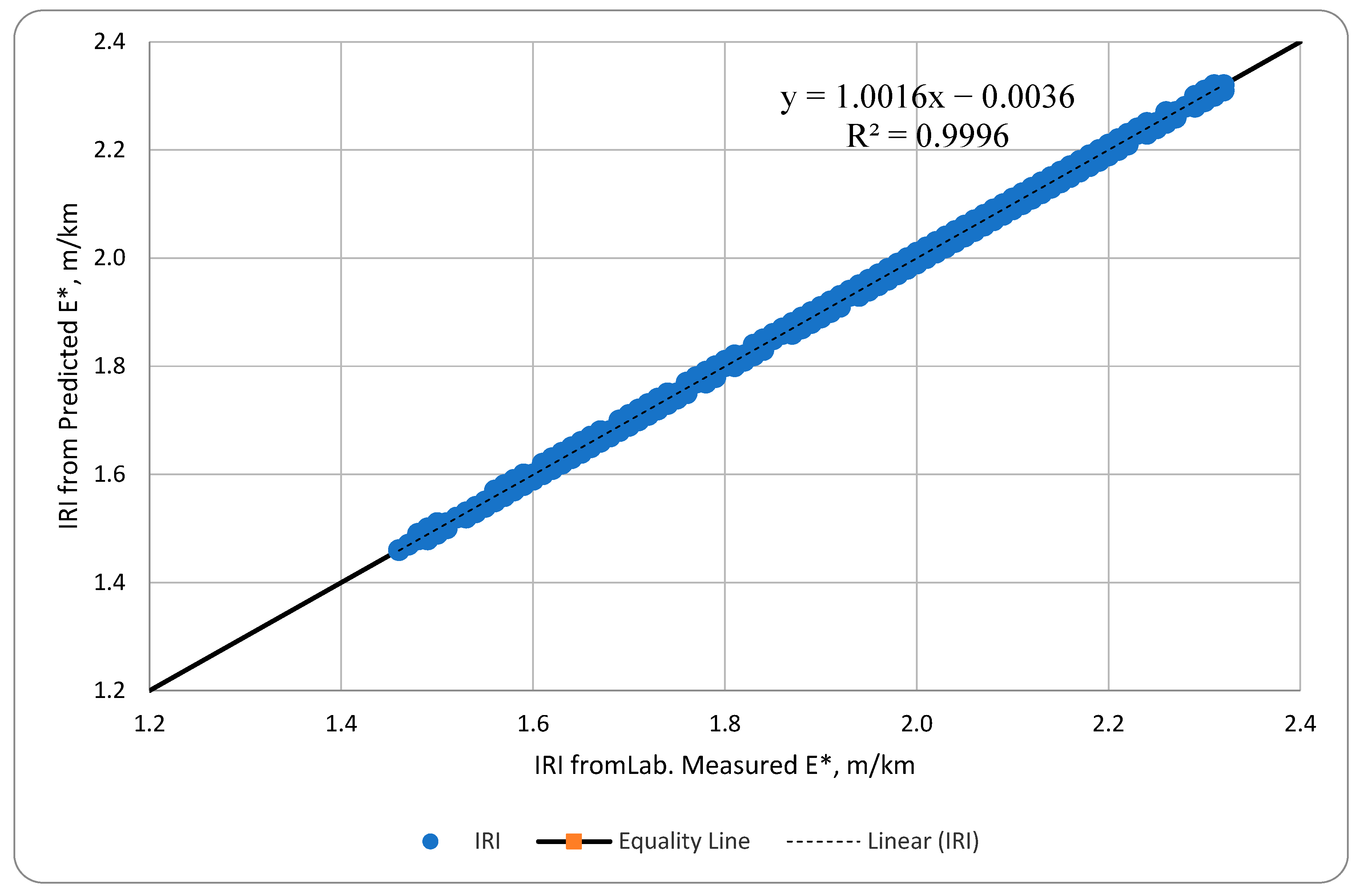
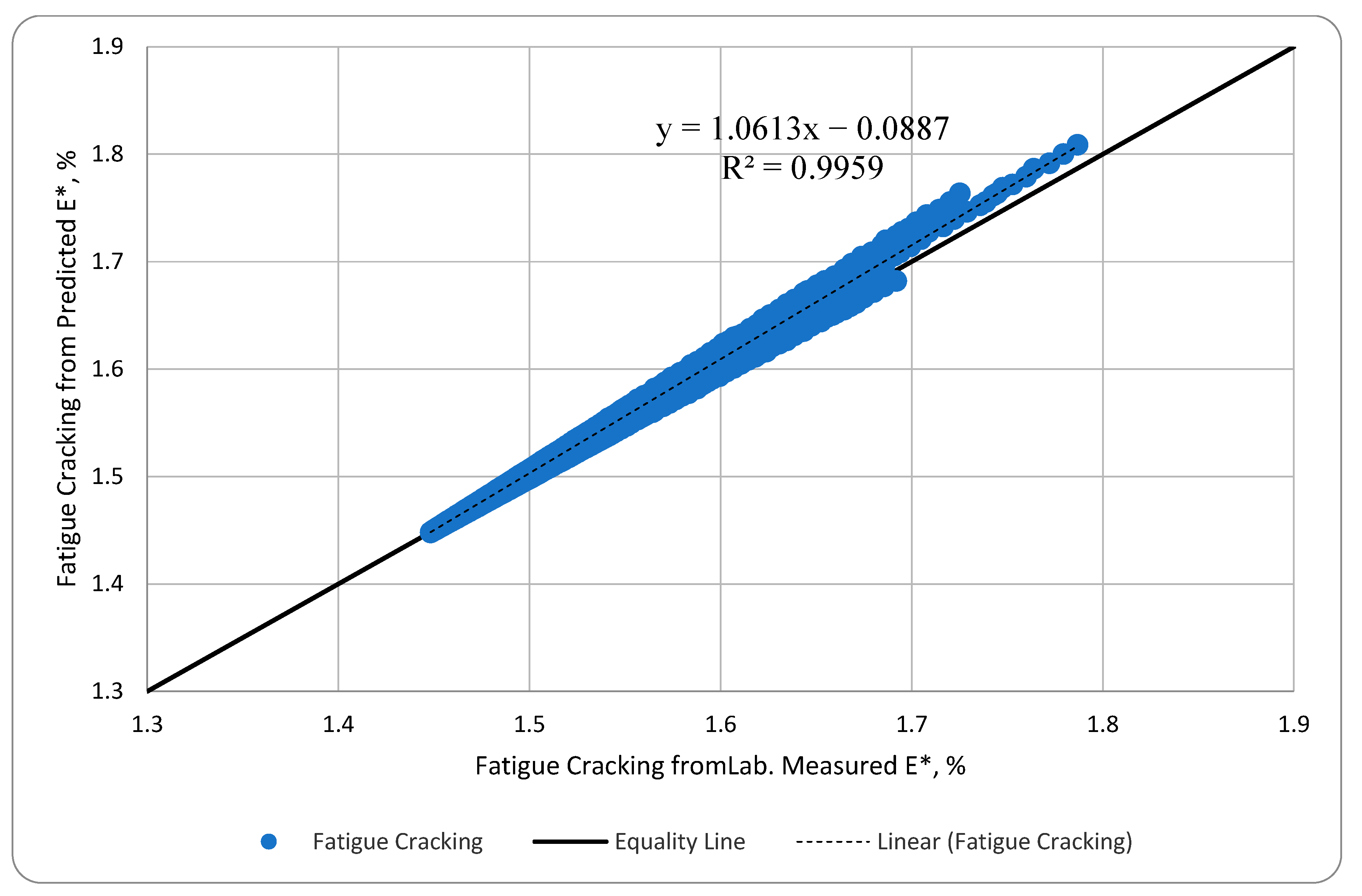
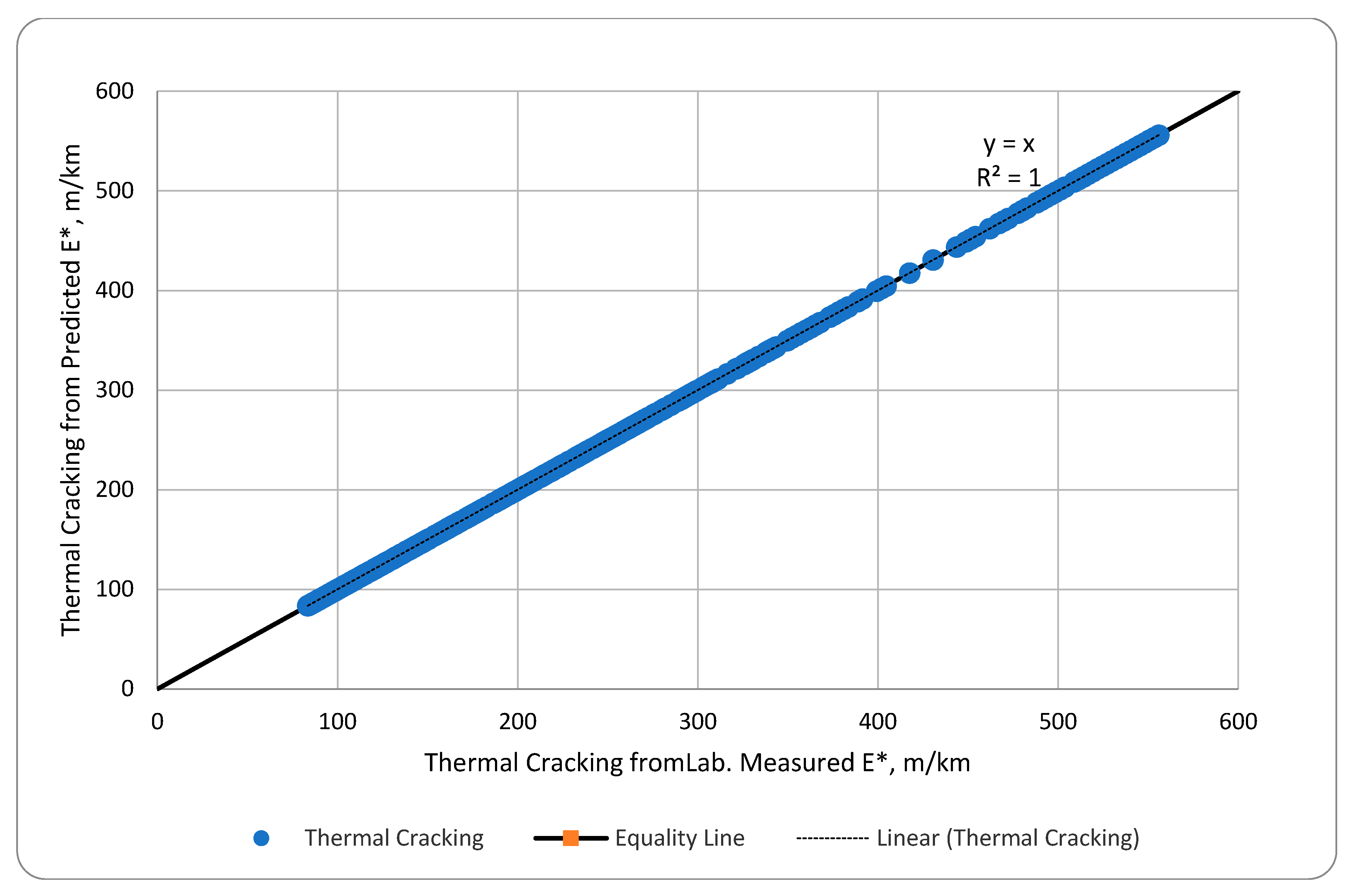
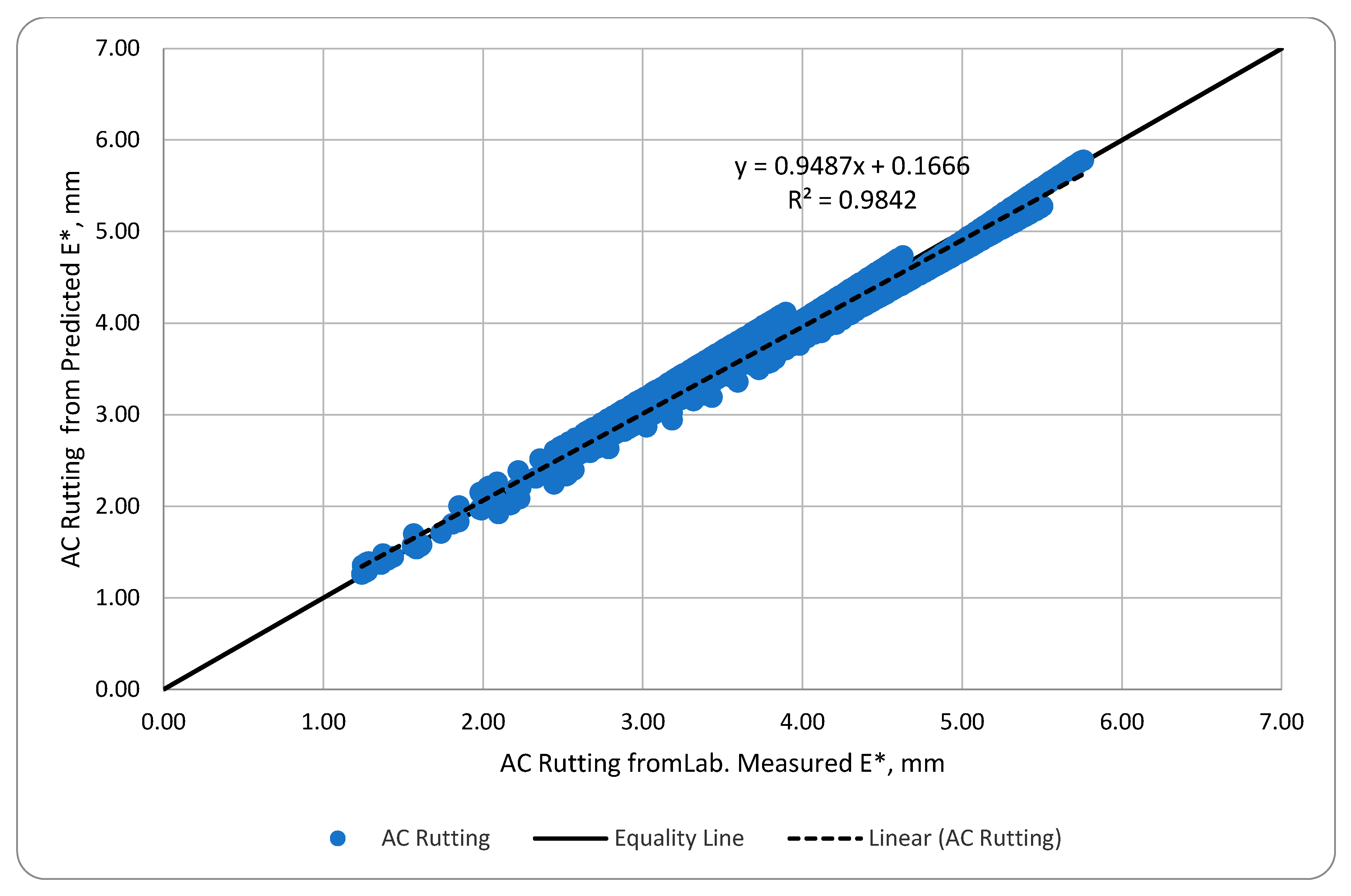
5.3. E*Prediction Effect on the AASHTOWare Pavement Performance Prediction

Since the NCHRP 1-40D prediction model was found to have a good prediction power in predicting the E* of the Egyptian HMA mixes, it was further assessed to study the effect of its predicted E* values on the pavement performance predicted by the AASHTOWare. The purpose of this analysis is to evaluate the difference in the prediction of distresses using both sets of data, i.e., the lab measured data and the NCHRP 1-40D model data. This comparison shows if there is a difference in the prediction of distresses between both sets of data. AASHTOWare Pavement ME predicts the performance of the asphalt pavement in terms of six performance indicators; IRI, FC, TC, LC, AC permanent deformation (R_AC), and the total permanent deformation (R_T). This was carried out by running different typical design cases (AASHTOWare simulation runs) using the E* predicted values from the NCHRP 1-40D model. Then, the same design cases were re-run again with the actual laboratory measured E* values instead of the E* predicted values. Consequently, the AASHTOWare Pavement ME performance prediction was investigated by comparing the six performance indicators from the measured E* to those from the predicted E* in reference to the equity line and coefficient of determination R² was calculated for the data points.

Typical design cases were specified to represent the typical Egyptian climatic conditions, traffic loading conditions, and pavement materials. Three different climatic zones were selected to represent the Egyptian hot regions (Aswan), moderate regions (Cairo), and coastal climate (Alexandria). Characteristics of the three climatic zones are shown in

Table 4. Climatic zones characteristics.

Zone	Latitude	Longitude	MAAT
Alexandria	31.2	29.9	19
Cairo	30	31.88	25
Aswan	24	33.75	26

.

A typical cross section composed of 5 cm asphalt surface layer (AC1), 13 cm asphalt binder course (AC2), and 30 cm granular base course (GB), as shown in Figure 6, was used to run the different design cases representing a typical cross section commonly used for high reliability roadway projects in Egypt. Different combinations of the surface layers and binder courses characterized in this current study were used for the above two layers: AC1 and AC2. Since ten plant-produced asphalt mixtures (six binder course and only four surface layer mixtures) were investigated for this study, only eight asphalt mixture combinations were used for AC1 and AC2 layers. For AC1 (surface layer) mixes 3, 6, 8, and 10 were used, meanwhile for AC2 (binder course), mixes 2, 5, 7, and 9 were used. The base layer had the following characteristics: granular materials with A-1-a classification, California Bearing Ratio (CBR) of 80%, and resilient modulus (Mr) of 357 MPa. This hypothetical section is resting on a subgrade soil of 10% CBR with AASHTO classification of A-2-6 and Mr of 92 MPa. The general inputs of the typical design cases were set to be a new flexible pavement classified as principal arterial designed at 90% reliability level for 20 years design period. It is worth mentioning that the analysis was comprehensive to include all the predicted pavement distresses all over the entire design period (20 years). This flexible pavement was designed for 12,949 Average Annual Daily Truck Traffic (AADTT), equivalent to about 70 MESAL (Million 80kN Equivalent Single Axle Load), representing an average of the traffic loads of the high reliability roadway classes in Egypt.

The dynamic moduli (E*) of eight different HMA mixes (four surface layer mixes and four binder course mixes) previously determined by both measuring in the laboratory and prediction using NCHRP 1-40D prediction model were used. Four different combinations of theses HMA mixes were used to run the AASHTOWare typical design case for three different Egyptian climatic zones (Cairo, Alexandria, and Aswan), as shown in Table 5. The three climatic zones were selected to cover a wide spectrum of variations of the Egyptian climate, as mentioned before. Accordingly, twenty-four different AASHTOWare simulation runs were conducted for the typical design case (three climate zones x four HMA mix combinations x two dynamic moduli inputs, measured and predicted). The outputs of these 24 simulations runs, in terms of the six AASHTOWare performance indicators, were used to assess the effect of the prediction of the E* on the estimated pavement performance by the AASHTOWare. Comparisons of the six performance indicators estimated with predicted versus measured E* are shown in Figure 7 through Figure 12. The main reason to compare the results of the AASHTOWare simulation runs with the measured E* values to the simulation runs results with the E* predicted values, illustrated in Figure 7 through Figure 12, is to study the effect of using the predicted E* values on the AASHTOWare prediction power for the different pavement performance indicators.

An excellent correlation of the IRI is shown in Figure 7 with R² of 0.9996. Fatigue cracking results are depicted in Figure 8 with R² of 0.9959. Since the calculation of the fatigue cracking is basically depending on the E*, this high R² of the fatigue cracking confirms that there is no significate effect of the predicted E* values on the fatigue cracking. The results of the thermal cracking with R² = 1, shown in Figure 9, is expected, since E* is not used directly to calculate the thermal cracking. The longitudinal cracking results shown in Figure 10 cope up with the other distresses’ results with high R² of 0.9946. The results of the permanent deformations, for either the asphalt concrete layers or for the whole layers, are shown in Figure 11 and Figure 12, respectively. The results from Figure 11 and Figure 12 prove that the E* has the highest effect on the rutting prediction of the pavement with the lowest R² of 0.9842 for the AC rutting and R² of 0.9945 for the total rutting. This was expected, since the rutting calculations are basically depending on the E* values. Hence, the high correlation (R² of more than 95%) of all the investigated pavement performance indicators predicted using the measured E* versus the predicted E* proves the high prediction power of the used E* model and confirms the insignificant effect of using the predicted E*, instead of the measured E*, on the AASHTOWare pavement performance.

Table 5. Different setups used to run the Typical Design Case by AASHTOware Pavement ME.

Setup No	Climate Zone	AC1 (Surface Layer) and AC2 (Binder Course) Combinations
1	Cairo	Mix 3 and Mix 2
2	Cairo	Mix 6 and Mix 5
3	Cairo	Mix 8 and Mix 7
4	Cairo	Mix 10 and Mix 9
5	Alexandria	Mix 3 and Mix 2
6	Alexandria	Mix 6 and Mix 5
7	Alexandria	Mix 8 and Mix 7
8	Alexandria	Mix 10 and Mix 9
9	Aswan	Mix 3 and Mix 2
10	Aswan	Mix 6 and Mix 5
11	Aswan	Mix 8 and Mix 7
12	Aswan	Mix 10 and Mix 9

Table 5. Different setups used to run the Typical Design Case by AASHTOware Pavement ME.

Setup No	Climate Zone	AC1 (Surface Layer) and AC2 (Binder Course) Combinations
1	Cairo	Mix 3 and Mix 2
2	Cairo	Mix 6 and Mix 5
3	Cairo	Mix 8 and Mix 7
4	Cairo	Mix 10 and Mix 9
5	Alexandria	Mix 3 and Mix 2
6	Alexandria	Mix 6 and Mix 5
7	Alexandria	Mix 8 and Mix 7
8	Alexandria	Mix 10 and Mix 9
9	Aswan	Mix 3 and Mix 2
10	Aswan	Mix 6 and Mix 5
11	Aswan	Mix 8 and Mix 7
12	Aswan	Mix 10 and Mix 9

Figure 7. IRI from the NCHRP 1-40D-predicted E* versus IRI from ab-measured E*.

Figure 7. IRI from the NCHRP 1-40D-predicted E* versus IRI from ab-measured E*.

Figure 8. Fatigue cracking from NCHRP 1-40D-predicted E* versus fatigue cracking from lab-measured E*.

Figure 8. Fatigue cracking from NCHRP 1-40D-predicted E* versus fatigue cracking from lab-measured E*.

Figure 9. Thermal cracking from NCHRP 1-40D-predicted E* versus thermal cracking from lab-measured E*.

Figure 9. Thermal cracking from NCHRP 1-40D-predicted E* versus thermal cracking from lab-measured E*.

Figure 10. Longitudinal cracking from NCHRP 1-40D-predicted E* versus longitudinal cracking from lab-measured E*.

Figure 10. Longitudinal cracking from NCHRP 1-40D-predicted E* versus longitudinal cracking from lab-measured E*.

Figure 11. AC rutting from NCHRP 1-40D-predicted E* versus AC rutting from lab-measured E*.

Figure 11. AC rutting from NCHRP 1-40D-predicted E* versus AC rutting from lab-measured E*.

Figure 12. Total rutting from the NCHRP 1-40D-predicted E* versus total rutting from lab-measured E*.

Figure 12. Total rutting from the NCHRP 1-40D-predicted E* versus total rutting from lab-measured E*.

Generally, Figure 7 through Figure 12 show that there is a good correlation between the results of the performance indicators predicted using the measured versus the NCHRP 1-40D predicted E* with R² (very close to the unity) ranges from 0.9842 (for AC rutting) to 0.9996 (for IRI). These results indicate that, for all practical purposes, the NCHRP1-40D E* prediction model can be used to predict E* of the Egyptian HMA mixes with no significant effect on the estimated performance/design using the AASHTOWare Pavement ME under different Egyptian climatic and traffic loading conditions.

6. Summary, Conclusions, and Recommendations

The performance of the NCHRP 1-37A and NCHRP 1-40D E* predictive models was investigated in this study using regionally produced HMA mixtures by comparing the values of the estimated E* versus the laboratory measured E*. The results showed that the NCHRP 1-40D predictive model had good performance, with high accuracy and low bias, compared to the NCHRP 1-37A predictive model and, hence, the NCHRP 1-40D model can be used to predict E* of the Egyptian HMA mixtures satisfactorily. Further assessment of the NCHRP 1-40D model took place by studying the effect of its predicted E* values on the pavement performance predicted by the AASHTOWare. The results showed that there was no significant effect of the predicted E* values on the AASHTOWare predicted pavement performance. Hence, the main conclusions can be summarized as follows:

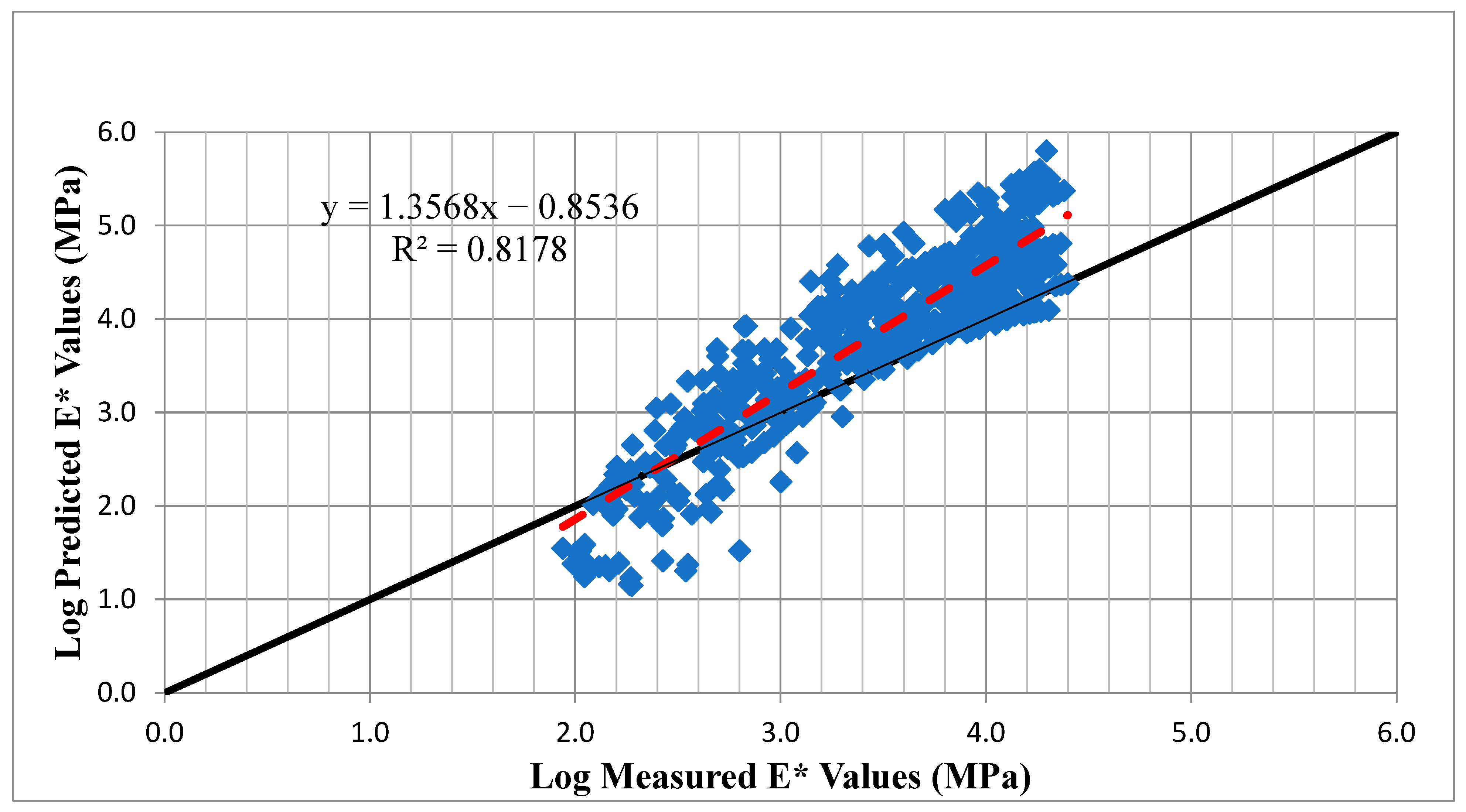
• The NCHRP 1-37A prediction model yielded poor E* predictions with high bias and high scatter for the Egyptian HMA mixes with a coefficient of determination (Adjusted R²) of 0.18 and S_e/S_y of 0.92 in the logarithmic scale. Thus, this model is not recommended to predict the E* for the Egyptian asphalt mixtures unless it is re-calibrated.
• The NCHRP 1-40D model yielded very good E* predictions with low bias and scatter for the Egyptian HMA mixes with an adjusted R² of 0.86 and S_e/S_y of 0.38 and, hence, it can be used satisfactorily to predict E* of the Egyptian asphalt mixtures.
• NCHRP 1-40D prediction model is recommended to regionally predict the Egyptian HMA mixes’ dynamic modulus, while the NCHRP 1-37A prediction model is not recommended for predicting the Egyptian HMA mixes’ dynamic modulus without further recalibration.
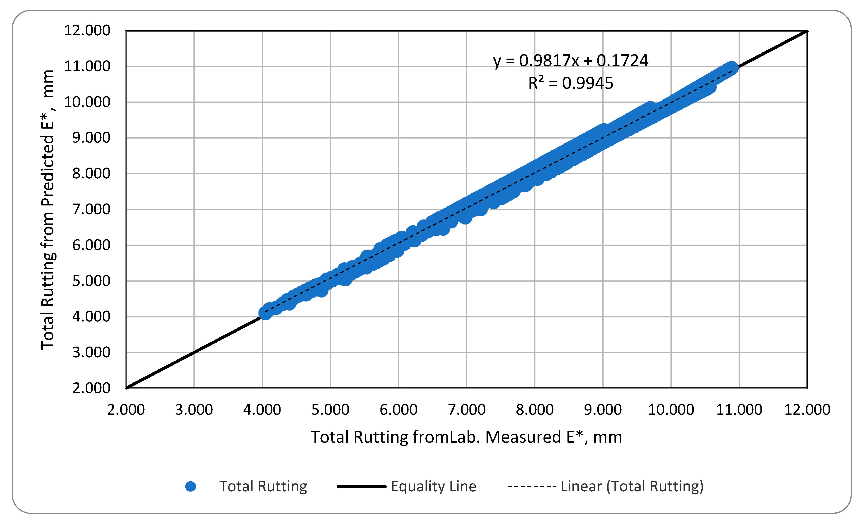
• The NCHRP 1-40D-model-predicted E* values have no significant effect on the AASHTOWare Pavement ME pavement performance prediction in terms of FC, TC, LC, R_AC, R_T, and IRI. Thus, the E* of the Egyptian HMA mixes can be satisfactory predicted using the NCHRP 1-40D-prediction model to be used as a material input in the AASHTOWare Pavement ME for the purposes of the design and analysis of the Egyptian flexible pavement.
• AASHTOWare Pavement ME design can be implemented regionally in Egypt to design and analyze flexible pavement provided that the Superpave grading system parameters (the complex modulus and the phase angle) of the asphalt binders are measured or fundamentally predicted using the A and VTS temperature-viscosity parameters to lead the software to predict the E* using the NCHRP 1-40D prediction model.

For further study, it is recommended to:

• Enlarge the database for the Egyptian HMA dynamic modulus considering all different varieties in the Egyptian pavement materials including more aggregate gradations and volumetric properties;
• Study the performance of the NCHRP 1-40D model in predicting the Egyptian E* using different types of modified asphalt binders;
• The NCHRP 1-37A E* prediction model needs to be calibrated for the Egyptian mixes;
• The AASHTOWare Pavement ME transfer functions to predict the pavement performance need to be validated and regionally calibrated.

References

1. AASHTOWare Pavement ME Design. Available online: https://www.aashtoware.org/products/pavement/pavement-me-design/ (accessed on 1 January 2021).
2. Khattab, A.M.; El-Badawy, S.M.; Elmwafi, M. Evaluation of Witczak E* predictive models for the implementation of AASHTOWare-Pavement ME Design in the Kingdom of Saudi Arabia. Constr. Build. Mater. 2014, 64, 360–369. [Google Scholar] [CrossRef]
3. ARA Inc. ERES consultants’ division. In Guide for Mechanistic-Empirical Design of New and Rehabilitated Pavement Structures; NCHRP 1-37A Final Report, Transportation Research Board; National Research Council: Washington, DC, USA, 2004. [Google Scholar]
4. Birgisson, B.; Sholar, G.; Roque, R. Evaluation of a predicted DM for Florida mixtures. J. Transp. Res. Board 2005, 1929, 200–207. [Google Scholar] [CrossRef]
5. Obulareddy, S. Fundamental Characterization of Louisiana HMA Mixtures for the 2002 Mechanistic-Empirical Design Guide. Master’s Thesis, Louisiana State University, Baton Rouge, LA, USA, 2006. [Google Scholar]
6. Azari, H.; Al-Khateeb, G.; Shenoy, A.; Gibson, N. Comparison of simple performance Test |E*| of accelerated loading facility mixtures and prediction |E* | use of NCHRP 1-37 A and Witczak’s new equations. J. Transp. Res. Board 2007, 1998, 1–9. [Google Scholar] [CrossRef]
7. Tran, N.H.; Hall, K.D. Evaluating the predictive equation in determining dynamic moduli of typical asphalt mixtures used in Arkansas. J. Assoc. Asph. Paving Technol. 2005, 74, 1–17. [Google Scholar]
8. Al-Khateeb, G.; Shenoy, A.; Gibson, N.; Harman, T. A new simplistic model for DM predictions of asphalt paving mixtures. J. Assoc. Asph. Paving Technol. 2006, 75, 1254–1293. [Google Scholar]
9. Christensen, D.W.; Pellinen, T.; Bonaquist, R.F. Hirsch model for estimating the modulus of asphalt concrete. J. Assoc. Asph. Paving Technol. 2003, 72, 97–121. [Google Scholar]
10. Andrei, D.; Witczak, M.W.; Mirza, W. Appendix CC-4: Development of a Revised Predictive Model for the Dynamic (Complex) Modulus of Asphalt Mixtures. In Development of the 2002 Guide for the Design of New and Rehabilitated Pavement Structures; Final document, NCHRP Project1-37A; Transportation Research Board of the National Academies: Washington, DC, USA, 1999; pp. 66–204. [Google Scholar]
11. Bari, J.; Witczak, M.W. Development of a new revised version of the Witczak E* predictive model for hot mix asphalt mixtures. J. Assoc. Asph. Paving Technol. 2006, 75, 381–424. [Google Scholar]
12. Flintsch, G.W.; Loulizi, A.; Diefenderfer, S.D.; Diefenderfer, B.K.; Galal, K.A. Asphalt material characterization in support of mechanistic-empirical pavement design guide implementation in Virginia. J. Transp. Res. Board 2008, 2057, 114–125. [Google Scholar] [CrossRef]
13. Dongre, R.; Myers, L.; D’Angelo, J.; Paugh, C.; Gudimettla, J. Field evaluation of Witczak and Hirsch models for predicting DM of Hot-Mix Asphalt. J. Assoc. Asph. Paving Technol. Proc. Tech. Sess. 2005, 74, 381–442. [Google Scholar]
14. Kim, Y.R.; King, M.; Momen, M. Typical Dynamic Moduli Values of Hot Mix Asphalt in North Carolina and Their Prediction, CD-ROM. In Proceedings of the 84th Annual Meeting, Washington, DC, USA, 9–13 January 2005; TRB: Washington, DC, USA, 2005. [Google Scholar]
15. Schwartz, C. Evaluation of the Witczak DM Prediction Model, CD-ROM. In Proceedings of the 84th Annual Meeting, Washington, DC, USA, 9–13 January 2005; TRB: Washington, DC, USA, 2005. [Google Scholar]
16. Pellinen, T.K.; Witczak, M.W. Use of stiffness of Hot-Mix Asphalt as a simple performance test. Transp. Res. Rec. 2002, 1789, 80–90. [Google Scholar] [CrossRef]
17. Singh, D.; Zaman, M.M.; Commuri, S. Evaluation of Predictive Models for Estimating DM of HMA Mixes Used in Oklahoma. In Proceedings of the TRB Annual Meeting, Washington, DC, USA, 23–27 January 2011. [Google Scholar]
18. Robbins, M.M.; Timm, D.H. Evaluation of DM predictive equations for southeastern United States asphalt mixtures. J. Transp. Res. Board 2011, 2210, 122–129. [Google Scholar] [CrossRef]
19. Moussa, G.S.; Owais, M. Pre-trained deep learning for hot-mix asphalt DM prediction with laboratory effort reduction. Constr. Build. Mater. 2020, 265, 120239. [Google Scholar] [CrossRef]
20. Behnood, A.; Golafshani, E.M. Predicting the DM of asphalt mixture using machine learning techniques: An application of multi biogeography-based programming. Constr. Build. Mater. 2021, 266, 120983. [Google Scholar] [CrossRef]
21. Xu, W.; Huang, X.; Yang, Z.; Zhou, M.; Huang, J. Developing hybrid machine learning models to determine the DM (e*) of asphalt mixtures using parameters in witczak 1-40d model: A comparative study. Materials 2022, 15, 1791. [Google Scholar] [CrossRef] [PubMed]
22. Daneshvar, D.; Behnood, A. Estimation of the dynamic modulus of asphalt concretes using random forests algorithm. Int. J. Pavement Eng. 2022, 23, 250–260. [Google Scholar] [CrossRef]
23. Huang, J.; Zhang, J.; Li, X.; Qiao, Y.; Zhang, R.; Kumar, G.S. Investigating the effects of ensemble and weight optimization approaches on neural networks’ performance to estimate the dynamic modulus of asphalt concrete. Road Mater. Pavement Des. 2023, 24, 1939–1959. [Google Scholar] [CrossRef]
24. Kim, J.; Byron, T.; Sholar, G.; Kim, S. Development of DM Testing and Data Interpretation Capability; Research Report FL/DOT/SMO/08-514; State Materials Office: Alachua County, FL, USA, 2008. [Google Scholar]
25. Clyne, T.R.; Li, X.; Marastenau, M.O.; Skok, E.L. Dynamic and Resilient Modulus of Mn/DOT Asphalt Mixtures; Final Report MN/RC—2003-09; University of Minnesota: Minneapolis, MN, USA, 2003. [Google Scholar]
26. Cho, Y.-H.; Park, D.-W.; Hwang, S.-D. A predictive equation for DM of asphalt mixtures used in Korea. Constr. Build. Mater. 2010, 24, 513–519. [Google Scholar] [CrossRef]
27. Mohammad, L.N.; Saadeh, S.; Obulareddy, S.; Cooper, S. Characterization of louisiana asphalt mixtures using simple performance tests. In Proceedings of the 86th Annual Meeting of the Transportation Research Board, Washington, DC, USA, 21–25 January 2007; TRB: Washington, DC, USA, 2007. [Google Scholar]
28. Awed, A.; El-Badawy, S.; Bayomy, F.; Santi, M. Influence of MEPDG binder characterization input level on predicted DM for idaho asphalt concrete mixtures. In Proceedings of the Transportation Research Board 90th Annual Meeting, Washington, DC, USA, 23–27 January 2011. [Google Scholar]
29. Georgouli, K.; Loizos, A.; Plati, C. Calibration of DM predictive model. Constr. Build. Mater. 2016, 102, 65–75. [Google Scholar] [CrossRef]
30. El-Badawy, S.; Awed, A.; Bayomy, F. Evaluation of the MEPDG DM prediction models for asphalt concrete mixtures. In Proceedings of the First Congress of Transportation and Development Institute (TDI), Chicago, IL, USA, 13–16 March 2011. [Google Scholar]
31. Far, M.; Underwood, B.; Ranjithan, S.; Kim, R.; Jackson, N. Application of artificial neural networks for estimating DM of asphalt concrete. In Transportation Research Record 2127; Transportation Research Board: Washington, DC, USA, 2009; pp. 173–183. [Google Scholar]
32. El-Badawy, S.; Bayomy, F.; Awed, A. Performance of MEPDG DM predictive models for asphalt concrete mixtures: Local calibration for idaho. J. Mater. Civ. Eng. 2012, 24, 1412–1421. [Google Scholar] [CrossRef]
33. Yousefdoost, S.; Vuong, B.; Rickards, I.; Armstrong, P.; Sullivan, B. Evaluation of DM predictive models for typical Australian asphalt mixes. In Proceedings of the 15th AAPA International Flexible Pavements Conference, Brisbane, Australia, 22–25 September 2013; pp. 22–25. [Google Scholar]
Figure 1. Research methodology.
Sustainability 15 14030 g001
Figure 2. Dynamic modulus (E*) master curves of binder courses.
Sustainability 15 14030 g002
Figure 3. Dynamic modulus (E*) master curves of surface layers.
Sustainability 15 14030 g003
Figure 4. The Predicted versus The Measured E* for NCHRP 1-37A Prediction Model.
Sustainability 15 14030 g004
Figure 5. The Predicted versus The Measured E* for NCHRP 1-40D Prediction Model.
Sustainability 15 14030 g005
Figure 6. Design case typical cross section.
Sustainability 15 14030 g006