Abstract
The paper focuses on secondary bio streams which are not captured efficiently in the value supply chain. Specifically, roadside grass clippings were chosen, based on their logistical optimization potential, direct feasibility, locality, biomass potential, and economic valorization value. The main objective is to determine how this secondary flow can be brought to the “factory gate”—through road transport and inland shipping—and at what cost per unit. To this end, various scenarios were developed for a case study in East Flanders, considering multiple combinations of first collection points, secondary collection points, and processing points. The result is a generically applicable Excel-based tool that combines these variations with a solution considering both inland waterways and road transport. These scenarios become valuable in applying the tool for grass clippings and optimizing this value chain located in East Flanders. The results show that reducing the number of collection points is favorable for the utilization of inland waterways, as it reduces costs related to transshipment. Nevertheless, unimodal road transport is still the most cost-effective method for transporting this secondary material stream from the collection point to the processing point. Consequently, a lower weight and a higher density will lead to lower costs, which eventually bottom out, due to regulations and conditions that must be met.
1. Introduction
This paper is based on the interest in implementing various optimized company processing technologies aimed at applying biomass flows to oils, fats, and lignocellulose-rich byproducts. The focal point of this paper is the efficient collection of roadside grass clippings, and it also investigates whether higher-quality valorization is possible. The main objective is determining how this secondary flow can be brought to the factory gate using road transport and inland shipping—and at what cost per unit.
The geographical scope of the illustrative case study is East Flanders (Belgium). Preliminary research on different use cases, considering biomass potential for the province of East Flanders, can be found in Ref. [1]. In expert meetings, it was decided to pursue the case of roadside grass clippings in East Flanders, considering multiple variables, such as (1) the logistical optimization potential, (2) the innovative processing chain, (3) direct feasibility, (4) the multiplicability in the market, (5) the East Flanders location, (6) biomass potential, and (7) the economic valorization value [1]. The project steering committee indicated there were already multiple projects active within this niche that could be linked to the project described in this paper.
To answer the main research question, two statements are validated. First, sensitivity analyses are used to investigate the effect of changes in several parameters on the cost—for instance, the effects of a change in density. Thus, an indication can be given of how transport can become more economically viable. The cost will be expressed in euros per ton, and hereafter, interested companies can compare the calculated cost (euro/ton) with their willingness to pay, i.e., minimizing costs. Secondly, within the logistics area, this study examines the way in which large amounts of biomass can be delivered to the place of processing (the factory gate) at an acceptable cost. The focus is on grass clippings obtained along the highways, regional roads (AWV management), and municipal roads. In Flanders, this results in approximately 70,000 tons of roadside grass clipping (wet matter) annually [2]. Figure 1 represents the density of tons of grass clippings per municipality.
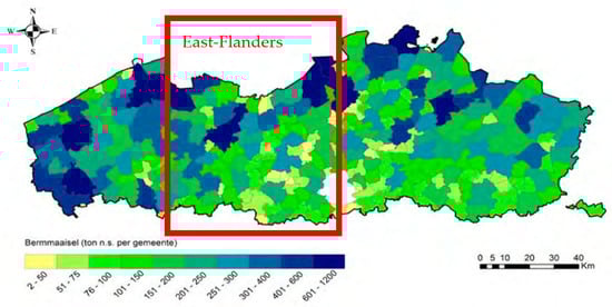
Figure 1.
Supply of roadside grass clippings per municipality (in tons) in Flanders—Source: [2].
This paper will elaborate on the collection and processing of grass clippings in Flanders. In general, the value chain is represented in Figure 2:

Figure 2.
Value chain overview—Source: own compilation.
The biomass is collected, sometimes stored, when the input exceeds the processing capacity [3], and brought to the factory. After processing, the secondary material is processed into a “known product” already on the market, initially produced using primary materials. Due to this economic landscape, it is only natural that competition occurs, and investigation is necessary to determine whether the “known product” can be produced using secondary material streams, i.e., the quality of the secondary material products, etc. must be evaluated.
The paper is structured as follows. Section 2 provides a brief overview of several studies on roadside grass clippings. Section 3 describes the case of roadside grass clippings in detail, analyzing the supply chain from numerous collection points to the processing plant, with several scenarios. Explanatory variables, formulas, and assumptions are used to calculate the cost, with an overview of this process in Section 4. Section 5 represents the calculated values per scenario, along with (interim) conclusions. Section 6 examines the potential impact of the cost of mowing roadside grass clippings and transporting them to the first collection point. Finally, Section 7 concludes with some possible further analyses.
2. Literature Review
In Flanders, several studies have been carried out (overview Table 1) on the processing of roadside grass clippings, with the main focus on fermentation and/or composting.
Due to the ever-growing population and urbanization, the generated secondary material increases consequently. Recycling this secondary material can be achieved in several ways. The required raw materials can be extracted and reprocessed, or they can be burned, recovering the heat by electricity-conversion [4]. The latter results in enormous amounts of pollution that cause environmental and health issues. Waste management, therefore, is the collection, transportation, processing, recycling, disposal, and monitoring of waste streams. Its goal is to reduce the amount of matter that enters and leaves society, while also encouraging the reuse of secondary material streams within society, with the following goals [5]: (1) reduce the total amount of waste by recycling and reducing the amount of waste generated, (2) re-introduce secondary raw materials or energy carriers into production processes, (3) re-introduce secondary raw materials back into their natural cycle, (4) dispose on suitable landfills, and (5) counter the fluctuations in waste quantities.
According to Ref. [6], the land use impact of energy crops has led the biogas industry to shift towards alternative side streams such as manure, food processing waste, and sewage sludge. Using these byproducts as biogas feedstock reduces GHG emissions from their conventional treatment pathways (landfilling, incineration, and composting) and generates “green” energy in the form of biogas/biomethane. Since roadside grass clippings are considered waste under the EU Waste Framework Directive (2008/98/EC), the highest valorization purpose of this sidestream, i.e., feedstock, cannot be produced. Therefore, only a tiny fraction is currently used for composting, or anaerobic digestion [7]. In 2021, 4.6%—or 18.6 billion cubic meters [8]—of the European gas requirements was fulfilled with biogas. The REPowerEU wants to increase the utilization of these sidestreams up to 35 billion cubic meters by 2030 [9]. In contrast, the IEA envisions an increase of up to 125 billion cubic meters by 2040 [10].
As explained within this paper, in addition to oils, several case studies utilize roadside grass clippings for energy production. Refs. [11,12] reflect on the challenges of transporting secondary organic material streams—specifically roadside grass clippings—in urban areas. One of the main drivers of greenhouse gas emissions in cities is the result of complex logistics in regards to dealing with pollution [13]. The presence of green grass strips is somewhat limited, dispersed, and fragmented compared to that of open agricultural areas, with about 65% of these strips under 0.1 ha [12].
The case study by Ref. [14] proves that joint collection, pre-processing, and conversion with other organic waste streams enable synergies. Considering the abundant waste streams available in Flanders (i.e., sludge and other organic waste), 20% of the renewable energy could be supplied in this province. Nevertheless, there are also challenges. The availability and handling of these wastes lead to significant fluctuations in the amount of secondary material that can be collected. These fluctuations are reflected in pricing. Pre-processing could densify the voluminous biomass and potentially reduce the logistics costs correlated with transporting the organic waste to its point of processing, while simultaneously tackling this uncertainty [15]. Alternatively, the long-term storage of organic waste after pre-processing at a central location could avoid supply fluctuations and enhance the filling rate of logistical streams, stabilizing irregular patterns [11,16].
Consequently, supply chain management and optimization of the different storage and processing points can stimulate the integration of the sector with other waste streams, creating an efficient bio-energy network throughout Flanders and the Benelux [17]. The integration of organic biostreams into a network will largely depend on the economic feasibility of this type of valorization. Although roadside grass clippings are a relatively cheap organic waste stream, they boast a low energy conversion efficiency and high transport and handling costs [18]. As such, HILD (high-input low-diversity) biomass or fossil fuels still hold the advantage.

Table 1.
The most important conclusions from the relevant studies conducted in Flanders.
Table 1.
The most important conclusions from the relevant studies conducted in Flanders.
| Source | Most Important Conclusions | |
|---|---|---|
| East Flanders | [19] | Logistical challenges are: seasonality, geographical spread, rapid degradation, required pre-treatment, pollution, and (only) 2 mowing periods. Quantities of clippings per year fluctuate considerably. Only the weighing at the processor is reported, meaning that the full supply is not known (in case grass clippings are mowed but not collected) Ideally, the roadside grass is ensiled or processed within ten days after harvest. |
| Flanders | [20,21] | “As far as the management of roadside grass is concerned, it has already been demonstrated that this represents a high cost for the responsible authorities. Not only mowing but also disposal and processing can be a financial obstacle.” |
| Alterra | [22] | Points of attention: Supply uncertainty, complex logistics, insufficient awareness of managers that they are raw material producers, tendering method, lack of clarity regarding which party in the chain should take control. |
| Bermg(r)as | [23] | The litter problem is essential in wet fermentation, but does not pose a problem with dry fermentation. |
| East Flanders | [24] | Uncertainty surrounding the storage costs, treatment cost, and processing price. Receiving correct volume data can be a problem regarding which the change from composting to fermentation can be a solution. Consequently, all the involved parties need to be in agreement. |
| Bermstroom | [25] | Roadside clippings for paper production: the increasing demand for e-commerce develops parallel to the increasing request for paper and cardboard shipping materials. The Flanders case is rather complex, since the local industry focuses on high-quality graph paper, which requires additional research [26]. Innovations regarding the different steps in the value chain were investigated during the project. This value chain includes the following steps: (1) mowing, (2) transport and storage, (3) paper production, and (4) closing the loop. |
| Grassification | [27] | Valorization of roadside clippings to create a value chain— the common challenges for processing roadside grass clippings are the following: supply (chain) is not optimal, resulting in high costs, grass clippings are heterogeneous in supply, and political challenges stemming from an unsupportive legal framework. |
| Economic potential of bio-streams | [28] | Main findings/limitation: Due to the local and widespread character of grass clippings, good logistical planning is crucial to mobilize and guarantee sufficient supply; there is no uniform quality standard in regards to all clippings; and the roadside grass clippings are not considered waste. Therefore, sufficient attention is not paid to the subject. |
A typical logistics chain of roadside grass clipping consists of several steps. First, the roadside grass is mowed, after which it is either temporarily stored/collected at a collection point or transported directly to a digester or composter. The monetary valuation of transporting goods between two points can be expressed in cost or price. For this paper, the decision was made to use both.
Nonetheless, the difference can be defined as follows: (1) the cost of transporting goods from A to B starts from the owner’s point of view in regards to the means of transport, i.e., the “out-of-pocket cost”; (2) the price for transporting goods from A to B starts from the point at which that the sender of goods does not have a means of transport. Therefore, the price for transport results from the market mechanism (supply and demand). In theory, this price can be higher or lower than the cost. The advantages of using cost or price are as follows: (1) in economic feasibility studies, it is possible to work with different levels of costs. For example, it is possible to check the effect of an increase in the price of diesel on the total cost of transport; (2) using prices is more convenient and less time-intensive, since these can be requested from transporters. However, available prices are a snapshot, prompting the need consult the price regularly during the research phase.
A distinction can be made between different cost items (The section of this report in which the corresponding information can be found is listed in parentheses). (1) The cost of mowing and collection at a first intermediate point (Section 6); (2) the transport from the first intermediate point to possibly a second intermediate point, after which it is further transported to the final processing point (Section 3); (3) the cost of storage/ensiling at the collection points (Section 6). The grass clippings can be stored either ensiled or in pressed round bales, with different costs borne by different stakeholders. The question, therefore, arises regarding which costs will be passed on to other parties. For example, it must be determined whether the mowing costs incurred (by the municipalities or the roads and traffic administration) will be passed on to the final processor. This paper focuses primarily on the relationship between the first collection point and the final processor.
3. Description of the Developed Scenarios
As a starting point, the results from the Grenzeloze Logistiek project were used to create a table including the theoretical estimate of tons of roadside grass clippings per mowing that could be collected per collection point. The case, therefore, starts from the assumption that roadside grass clippings have already been gathered at a collection point. Table 2 and Figure 3 provide an overview of the tonnages of roadside mowing clippings per collection point. This overview represents a hypothetical case, since the reported tonnages also contain roadside grass clippings from municipalities not collected at the identified collection points that day, but also from those transported directly to a digester or composter [1,24]. The allocation of the collection points is based on the parameter distance [1].
Table 2.
Tonnage of roadside grass clippings per collection point (East Flanders), from both regional and municipal roads, 2010. Source: [19].

Figure 3.
Overview of collection points (left) and storage points (rights): collection points in East Flanders—Source: own compilation.
Table 2 reflects the 41 different storage points pinpointed within Figure 3. These locations are in East Flanders. The Table furthermore states the names of that storage point, i.e., X + number storage point, and the storage capacity (in tons of wet clippings). The total value refers to the total number of tons of wet matter stored at the 41 storage points.
Figure 4 represents the demarcation of the analysis in this part of the report. The starting points are several first storage points/collection points for roadside grass clippings (X). Consequently, the clippings are transported to intermediate locations (Y), with the final destination being the place of processing (Z). In the elaborated scenarios, the assumption is made that there is only one place of processing.
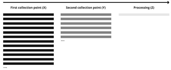
Figure 4.
Focus research regarding roadside grass clippings—demarcation analysis. Source: own compilation.
A total of five scenarios will be studied. An overview is given in Table 3, and it is subsequently briefly described. The mode of transport of the first three scenarios is road transport, while the last two scenarios considered both road transport and inland navigation modes. Furthermore, the number of first collection points (X) and the second collection points (Y) vary. The fifth scenario determines an optimal processing location (Z).
Table 3.
Overview of scenarios. Source: own compilation.
3.1. Scenario 1
In Scenario 1, the cost is calculated for the transport of roadside grass clippings from 41 collection points (X, spread over East Flanders) (Figure 5) to one processing plant (Z, Kluizendok Haven Gent) (see Figure 6), with the help of road transport. No intermediate storage place was utilized in this scenario.
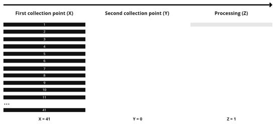
Figure 5.
Scenario 1: chain structure. Source: own compilation.

Figure 6.
Scenario 1: location of final processing. Source: own compilation.
3.2. Scenario 2
Scenario 2 (schematically presented in Figure 7) investigates how the transport cost changes if four intermediate storage locations are chosen for pre-treatment of the roadside grass clippings. Figure 8 presents the division of the 41 collection points into four groups (i.e., demarcation within the circles). For each group, the roadside grass clippings are transported to an intermediate point, highlighted in green. The division into four groups is performed manually, without any specific criterium.

Figure 7.
Scenario 2: chain structure. Source: own compilation.

Figure 8.
Focus research on roadside grass clippings—demarcation analysis of Scenario 2. Source: own compilation.
3.3. Scenario 3
Instead of opting for 41 collection points, fewer storage spaces can also be used. Scenario 3 selects nine repositories and, as in Scenario 1, examines the effects of changing variable values. Figure 9 shows that no second collection points (Y) are selected; thus, the grass clippings are directly transported to the processing plant (Z). Figure 10 visualizes the demarcation analysis within East Flanders, with the nine collection points marked in green.

Figure 9.
Focus research of roadside grass clippings—demarcation analysis Scenario 3. Source: own compilation.

Figure 10.
Focus research on roadside clippings—demarcation analysis Scenario 3. Source: own compilation.
3.4. Scenario 4
In the previous scenarios, a truck was always used to arrange the transport of roadside grass clippings. This scenario investigates to what extent the use of an inland waterway vessel might lead to a change in the total transport costs. The clippings are transported from the 41 storage sites to a transshipment point beside the water (Figure 11). Afterward, the roadside grass clippings are transported to a processing plant near the water.
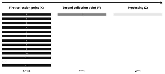
Figure 11.
Focus research regarding roadside grass clippings—demarcation analysis Scenario 4. Source: own compilation.
3.5. Scenario 5: Optimization
In the above scenarios, predetermined origins and one destination were used. In Scenario 5, the optimal location in Flanders for a processing plant is determined, and this selection is elaborated in Section 5.5.
4. The Calculation Tool
For further analysis, a newly developed and generically applicable calculation tool was developed based on the Excel file so that other users could make independent calculations. The tool allows for dealing with various modes of transport and their combinations, as is also required for dealing with the various scenarios identified in Section 3. Table 4 and Table 5 list all the variables and formulas used, elaborating on several typical logistics characteristics (such as tonnage, volume, location, distances, and travel times) and specific product characteristics for transport (such as density and conversion factor). These variables and formulas are used to determine the transport cost of getting the goods to the processing site. Even though kilometer costs are less appropriate for the cost calculations for inland shipping, it is still used to create consistencies between the employed road transport and inland shipping.
Table 4.
Variables used in the analysis. Source: own compilation.
Table 5.
Formulas used in the analysis. Source: own compilation.
A distinction is made between compacting and dewatering. Compaction means that the density is adjusted without a weight change. The effect of compacting is introduced by changing the value fx (density). Dewatering means that the weight is changed through dewatering. The effect of dewatering is introduced by changing the value e (the possible weight reduction in %). The weight reduction cannot lead to a weight lower than the dry matter weight, which is expressed by the value g. The conversion factor g shows how much the dry matter content is based on the tonnage of wet matter as it was initially delivered. In addition to defining a trip, it is necessary to define which vehicle will be used during transport. The input parameters associated with the vehicle implemented in the model are (1) the loading capacity in tons and m3, (2) the transport cost parameters, and (3) the loading and unloading time (see Table 6).
Table 6.
Cost factors including cost per kilometer and hourly cost. Source: [29].
Certain assumptions were used in the analyses. For example, the analysis of the transport is limited between point X and a destination (Y or Z); no analysis is performed regarding the bundling of multiple collection points before driving to the final destination. In order to be able to perform the analysis, it is assumed that there is no pre- and post-transport to reach location Y or Z. The kilometer and hourly costs are based on the study in Ref. [29]. This study determined the prices, i.e., costs in 2011, for a tractor-trailer combination carrying 24–28 tons of payload. This data was then used as a starting value. A further breakdown of the kilometer and hourly costs is included in Table 6.
Table 7 contains guide values that can be used to indicate the cost of kilometers and hours.
Table 7.
Guide values for kilometers and hourly costs per type of vehicle (1 January 2015). Source: own calculations based on [29,30].
Considering the above characteristics, a tool was developed to replicate the logistics between two points using a specific truck. A distinction can be made between five different blocks included in the online tool, namely; (1) trips, (2) vehicle parameters, (3) load parameters, (4) results, and (5) contact. In the following paragraphs, these different blocks will be further explained.
4.1. Trips
The first block combines the necessary origin and destination combinations, adding these to a list (forming an origin-destination matrix). A trip consists of the following elements that form an input for the user: (1) the starting point (name with starting values X1), (2) the endpoint (name with starting values Y1), (3) the tonnage that needs to be transported (expressed in tons of wet grass clippings), (4) the covered distance (in Km), (5) the average speed of the truck (in Km/u), and (6) the option to include a return trip in the calculations (yes or no).
By clicking the add trip button, the trip(s) will be added to the list, which can be extended virtually infinitely. By clicking the erase trip button, it is possible to erase specific trips from the list. If the input values are not correctly formatted, an error message will occur on the screen, indicating what is wrong.
4.2. Vehicle Parameters
In addition to defining a trip(s), defining which vehicle will be used during the transport significantly impacts the model’s outcome. Therefore, the input vehicle parameters consist of the loading capacity in tons and m3, the transport cost parameters, and the loading and unloading time. By default, the Excel tool includes predefined values that can be adjusted to the user’s needs. Additionally, a reset button resets the quantities back to the default values.
4.3. Load Parameters
The third and last input block refers to the transported load parameters, consisting of the (1) load density, (2) weight reduction, and (3) conversion factor from dry to wet matter. Again, the load parameters have a default value set by the Excel tool. These parameters are all adjustable to the user’s needs. A reset button can reset the parameters to the default value(s).
4.4. Calculation Module
The last part of the Excel tool is the calculation block. This block will calculate different parameters based on the added trips, vehicle, and load parameters. The calculated (intermediate) parameters are the following: (1) average cost per ton (dry and wet matter), (2) total number of trips, (3) total covered kilometers, and (4) total transport cost to fulfill all added trips. The compound cost will be calculated for all selected trips by clicking the button to calculate the total. Again, it is possible to click the reset button to clear the values in this module.
4.5. Contact Module
The contact module makes it possible to provide feedback, ask questions, and leave comments or remarks to the site developers and the project manager. This block contains the following parameters: (1) name, (2) e-mail, and (3) questions or remarks.
5. Scenario Results
The following subsections calculate the possible values per scenario of the cost to transport the roadside grass clippings to the factory gate. First, the reference values are shown, leading to a transport cost for the reference scenario. In addition, a sensitivity analysis is elaborated, enabling the effect on the transport cost to be shown after a change in a variable’s value. Finally, the main conclusions are formulated. A distinction is always made between the transport cost based on the original wet and dry weights.
5.1. Scenario 1
Scenario 1 calculates the transport cost of roadside pulp from 41 collection points (spread over East Flanders) to one processing plant (Kluizendok Haven Gent). This supply chain starts with the reference values denominated in Table 8. The variables—maximum volume and load to be transported—are specific for the number of trucks used. Hereby, the assumption was made that the empty return journey is included in the cost calculation.
Table 8.
Reference values for Scenario 1 (road transport). Source: own calculation.
Table 9 departs from roadside grass clippings with a density of 0.22 ton/m3 for grass silage. In the case of round bales, this value is obtained in the range between 0.15 and 0.90 [19]. The reference scenario states that when transporting 9841 tons of wet roadside clippings from the 41 collection points to a location in the Kluizendok (Port of Ghent), a total transport cost of EUR 106,002 is obtained. This scenario corresponds to EUR 10.77 per ton of wet matter or EYR 44.29 per ton of dry matter (based on a conversion factor of 24.32%). Table 9 shows a sensitivity analysis of these results by changing one variable at a time. Several changes to the basic assumptions are implemented:
Table 9.
Calculated values for Scenario 1 (9841 tons of wet grass clippings). Source: own calculation.
- -
- The cost per kilometer (e.g., by entering the road pricing or a higher fuel cost);
- -
- The hourly cost (e.g., due to an increase in the hourly wage of the driver);
- -
- The weight reduction of the grass clippings at the collection point;
- -
- The density of the roadside grass clippings at the collection point;
- -
- The load capacity of the truck in tons;
- -
- The loading volume of the truck in m3;
- -
- The collection distances;
- -
- The empty return trip is not considered (e.g., in case a return flow can be found).
Table 9 starts from the assumption that the transport is carried out by vehicles owned by the initiator. If the initiator does not own a fleet, a logistics service provider must be used to fulfill the logistics activities.
Based on the calculated values in Table 9, it can be observed that:
- (1)
- A higher cost per kilometer makes the collection of roadside clippings more expensive. An increase in the cost of fuel increases the logistics cost of collection. Road pricing will also increase this cost, depending on the route (where payment must be made). Introducing road pricing in regards to the main roads will likely have a relatively small impact.
- (2)
- A higher hourly cost also increases the logistics costs, i.e., by increasing the driver’s wage costs.
- (3)
- A weight reduction at the collection points can significantly decrease logistics costs because the number of transport movements decreases. A weight reduction of 50% leads to a 49% reduction in logistics costs. This cost reduction must be compared with the extra costs needed to obtain this weight reduction at the individual warehouses. These additional costs are case-specific, and are not incorporated in this paper.
- (4)
- A decrease in transport movements also leads to a decrease in transshipments, thus decreasing transshipment costs.
- (5)
- The density of roadside grass clippings is an essential secondary condition for transport. A density of 0.22 tons per m3 was used as a default value, representing that the volume restrictions, and not the tonnage, will determine the number of trucks required. If one succeeds in increasing the density from 0.22 to 0.45 tons per m3, this will lead to a cost reduction of 50%. Densities higher than 0.45 do not reflect in additional cost reductions.
- (6)
- An increase in the load factor of the trucks has no effect, due to inherent volume limitations.
- (7)
- The logistics costs naturally increase if the distance between the collection points and the processing plant is higher (i.e., not in the Port of Ghent area). It is, therefore, essential to check whether a more optimal processing location can be determined. The determination of an optimal location is examined in Scenario 5.
The above calculations show that it is possible to reduce logistics costs when parameters, such as weight reduction and the density of roadside grass clippings, change. The difference then provides an idea of the cost of pre-treatment that one wishes to pay—at maximum—to achieve the weight reduction or the density change at the 41 locations. A 50% decrease in weight leads to a decrease in transport costs of EUR 52,003. This EUR 52,003 budget can be used to realize the parameter changes. Alternatively, these savings can be used to encourage technological developments.
5.2. Scenario 2
The calculations for Scenario 1 (41 collection points and one processing location) show that a weight reduction leads to a significant decrease in transport costs. The realization of a weight reduction comes with a cost, and this action must be carried out at 41 locations. It may, therefore, be advisable not to carry out this weight reduction at the 41 locations, but rather at only a few locations. Scenario 2 investigates how the transport cost changes if four intermediate storage locations are chosen, at which pre-treatment can occur. The results are reflected in Table 10.
Table 10.
Calculated values for Scenario 2 (9841 tons of wet grass clippings; road transport). Source: Own calculation.
An extra transfer point naturally implies an extra transshipment, resulting in a higher transport cost. Without a (further) weight reduction, the transport costs increase by no less than 45%, up to EUR 153,787. Continuing analysis of the decrease in transport costs compared to the reference scenario is vital. In other words, the weight reductions and/or density changes to employ must be determined. The calculations show that a minimum weight reduction of 40% must be achieved before a system with four intermediate points can become feasible, depending on the technology costs to achieve this weight reduction.
5.3. Scenario 3
Instead of opting for 41 storage locations, selecting fewer collection points is possible. Scenario 3 assumes nine repositories and examines, in parallel with Scenario 1, the effects of changing variable values. The reduction in the number of warehouses (from 41 to 9) leads to a cost reduction of EUR 17,727, which seems relatively low (Table 11). This cost decrease must be weighed against the cost of collecting the roadside clippings. The same conclusions as those determined in Scenario 1 apply here as well, but with the understanding that the total transport cost is now consistently lower.
Table 11.
Calculated values for Scenario 3 (9841 tons of wet grass clippings; road transport). Source: own calculation.
5.4. Scenario 4
In the previous scenarios, the primary and only mode of transport was over the road via a truck. Scenario 4 examines to what extent the use of a barge leads to a change in the total transport costs. The volumes are transported from the 41 warehouses to a transshipment point near the water (i.e., Oudenaarde), continuing transport to the Port of Ghent (Figure 12). The calculations assume an inland waterway vessel with a load capacity of 2000 tons and 2840 m3 (71 × 10 × 4). The reference values used are included in Scenario 4.

Figure 12.
Inland navigation network in Flanders. Source: Promotie Binnenvaart Vlaanderen.
Table 12 summarizes the reference values for Scenario 4. Compared with the reference values derived from the literature for the hourly cost, it is striking that the value used here is relatively low. This is primarily due to the sharp decrease in the purchase price of an inland waterway vessel. As a result, the capital cost (and, therefore, the hourly cost) is relatively low.
Table 12.
Reference values for Scenario 4 (road transport and inland shipping). Source: own calculation.
Based on the calculations in Table 13, using inland shipping is not an interesting option.
Table 13.
Calculated values for Scenario 4 (9841 tons of wet roadside grass clippings; road and inland shipping). Source: own calculation.
5.5. Scenario 5: Optimization
In the four previous scenarios, several predetermined origins and one (final) destination, i.e., the Port of Ghent (Kluizendok) apply. In Scenario 5, whether or not this final destination location can be optimized is evaluated. As a first step, the research area is demarcated, in which the location for a new processing plant was sought. A rectangle is drawn over Flanders to model the maximum limits which can be used when determining the research area. The coordinates from Table 14 are used to form the search area, which is graphically represented in Figure 11 (north latitude; east longitude):
Table 14.
Coordinates research area for Scenario 5. Source: own compilation.
The region from which the selection points could be selected is demarcated by the rectangle coordinates represented in Figure 13. Afterward, working with steps of 0.2 (degrees), 45 destinations, or 1845 origin-destination pairs, were determined for be examination. For this set of destinations, the calculations were executed to gain insights into the destination with the lowest transport costs, which was then dubbed the optimal location. This location was then assigned the index of 100, and it is represented in Figure 14. Alternative scenarios are represented in Figure 15, Figure 16, Figure 17 and Figure 18, each with higher indexes than that of the optimal destination. Each index point above 100 represents one percentage of extra transport cost for that destination. An overview of the different locations can be found in Table 15, with a visual representation in Figure 14, Figure 15, Figure 16, Figure 17 and Figure 18.

Figure 13.
Demarcation of the research area in Scenario 5. Source: own compilation.

Figure 14.
Location 1 (index 100). Source: own compilation.

Figure 15.
Location 2 (index 101). Source: own compilation.

Figure 16.
Location 3 (index 114). Source: own compilation.
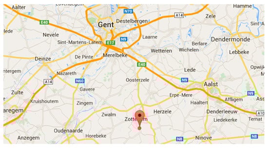
Figure 17.
Location 4 (index 116). Source: own compilation.

Figure 18.
Location 5 (index 120). Source: own compilation.
Table 15.
Overview of optimal locations. Source: own compilation.
For each set and each relationship, distances and travel times are calculated via Google Maps. The only difference noted when using the method in the above scenarios is that Google Maps reports travel times and distances based on passenger cars, not trucks. For this purpose, a correction factor is built in for the travel times: (1) if the distance is less than 20 km, the travel time is calculated based on an average speed of 50 km/h; (2) if the distance is greater than 20 km, the travel time is calculated based on an average speed of 65 km/h. The total transport cost is calculated per set of observations using the parameters reported in Scenario 1.
6. Additional Costs
In the logistics supply chain for the processing of roadside grass clippings, surplus costs in addition to the transport cost need to be added. A distinction can be made between mowing and first collection costs, storage costs, and gate fees. Figures were collected for each of these cost items.
6.1. Mowing and First Collection
Relevant information regarding the exact cost of mowing and collecting is scarce. The costs for a number of municipalities for mowing and collecting roadside grass can be found in the city council minutes. Table 16 was created based on a limited sample taken from a number of municipalities. This limited sample shows the importance of the financial cost to the municipality. In the calculations in Ref. [24], the share of the mowing cost amounts to 75% of the total logistics cost.
Table 16.
Cost to the municipality for mowing, suction, and disposal of roadside grass (sample). Source: own composition.
6.2. Storage
Ref. [32] states that storage must meet two conditions. First, it must be conditioned and controlled, i.e., after mowing, the microbiological degradation of the grass clippings should be controlled so that they can be stored to preserve the quality for further processing [32]. Secondly, the pre-treatment and the type of processing must be coordinated. Two methods of storage are distinguished: storage as pressed bales, and storage in a pit. A comparison of the cost of the different silage methods was carried out by Ref. [32]. The following values are reported per method:
- -
- Pit: EUR 5.2925/ton;
- -
- Slot silo: EUR 7.7125/tonne to EUR 9.8743/tonne;
- -
- Slurfsilo: EUR 8.0926/ton;
- -
- Wrapped bales: EUR 40.09/tonne.
6.3. Gate Fee
In the case of composting and digestion, a “gate fee” is mentioned, i.e., the amount paid to the roadside grass processor (based on the tonnage as delivered). In the case of composting, costs between EUR 30 and EUR 70 are reported [19,32].
6.4. Total Cost
Based on the previous sections, a determination of the relevant costs for the logistics of processing roadside grass clippings can be made. Consequently, it will be essential to know who will bear certain costs. In Table 17, it is assumed that the cost borne by the municipality or the roads and traffic agency will not be important in determining the cost of getting the roadside mower to the factory gate. Only the transport and storage costs, as determined in part 3, must be considered in that case.
Table 17.
Relevant charges in determining the total logistics costs. Source: own compilation.
Based on the calculations in Table 17, the roadside grass clippings can be delivered to the factory gate at a cost of between EUR 7/ton and EUR 55/ton for the new market player. These costs can then be checked with the willingness of the processor of the roadside grass clippings, on the one hand, to pay, and on the other hand, the current costs incurred for mowing roadside grass. The analysis distinguishes three parties that may have an interest in a new valorization of roadside grass clippings: (1) road managers (municipality or AWV), (2) waste processors, and (3) new market parties that are responsible for the organization of the roadside between the collection points and the new waste processor.
7. Conclusions and Discussion
This paper was motivated by the interest in implementing various optimized company processing technologies for applying biomass flows to oils, fats, and lignocellulose-rich byproducts. The focal point of this paper was the efficient collection of roadside grass clippings, and it also investigated whether a higher-quality valorization is possible. The main objective was to determine how this secondary flow could be brought to the factory gate—using road transport and inland shipping—and at what cost per unit. A generic cost model was developed to verify this assumption, including transport costs and logistics optimization elements. The model was applied to various scenarios for the East Flanders case study in Belgium.
The case study analysis shows that the supply chain for roadside grass clippings can be optimized based on the scenarios described in this paper. First, unimodal transport over the road is the most efficient method, leading to the lowest logistics cost. Extra transshipment locations generally lead to higher logistics costs, as can be noticed in Scenario 2. Therefore, reducing the number of primary locations can have a positive impact, considering the extra costs needed to transport the secondary material stream to the reduced number of transshipment points. Furthermore, alternative parameters, such as density and weight, were also researched. The conclusion is that a weight reduction, with a higher density, leads to lower logistics costs.
Nevertheless, these efficiency gains bottom out at ±45% due to various conditions that must be met, i.e., the maximum weight or maximum volume to be transported simultaneously. Looking at the supply chain, it becomes clear that there should be only one processing point. Questions arise about whether this processing location can be chosen more strategically. Section 5 develops an optimization approach based on the lowest transport cost for various destinations. Aside from the previously mentioned costs, additional costs such as gate, stocking, and mowing fees, should not be neglected. These costs are case-specific, and a good distribution of these costs between stakeholders should be negotiated. The above are findings that operators and policymakers should consider when developing secondary flow solutions, tailoring, of course, the magnitude of impacts to their specific settings by adapting the parameter values used in the model.
Specifically for the Flemish case study, an inventory of roadside grass clippings in Flanders was drawn. As a result, a database and an overview map of Flanders, including the production data regarding grass clippings, are shown. The inventory report includes the persons/agencies/associations contacted. If further analyses are required regarding the level of the production of roadside pulp in Flanders, it is best to start with data gathered from the Flemish Waste Management Agency (OVAM), or the municipal roadside, beginning with the analysis and the contact persons mentioned in the Graskracht study (2012) [20,21].
More generically, several parameters in the developed tool were adjusted in the above scenarios to calculate the new transport cost. This calculated transport cost can be checked with the processor’s willingness to pay. It is also possible to start from the processor’s willingness to pay and determine which values the underlying parameters must meet. As is the case regarding the processor’s respective willingness to pay, the parameters for other concrete settings can also be estimated.
Author Contributions
Conceptualization, F.D.W., T.P. and T.V.; Writing—original draft, J.W.; Writing—review & editing, C.S., E.V.d.V., E.v.H. and T.V. All authors have read and agreed to the published version of the manuscript.
Funding
This research was funded by IWT Vlaanderen under grant number 100938.
Institutional Review Board Statement
Not applicable.
Informed Consent Statement
Not applicable.
Data Availability Statement
No additional data apart from the ones shown in the main text are available.
Conflicts of Interest
The authors declare no conflict of interest.
References
- Devriendt, N.; Van Dael, M.; Van Roye, K.; Speijer, F. Haalbaarheidsanalyse Business Cases en Opmaak van Business Plannen Met Betrekking tot Logistieke Optimalisatie van Bio-Restromen; VITO: Lier, Belgium, 2014. [Google Scholar]
- OVAM. Aanbod en Bestemming Biomassa(rest)stromen Voor de Circulaire Economie in Vlaanderen; OVAM: Mechelen, Belgium, 2017. [Google Scholar]
- GR3. Grass as a Green Gas Resource: Energy from Landscapes by Promoting the Use of Grass Residues as a Renewable Energy Resource; Flemish Government: Brussel, Belgium, 2014.
- Demirbas, A. Waste management, waste resource facilities and waste conversion processes. Energy Convers. Manag. 2011, 52, 1280–1287. [Google Scholar] [CrossRef]
- Kan, A. General characteristics of waste management: A review. Energy Educ. Sci. Technol. Part A Energy Sci. Res. 2009, 23, 55–69. [Google Scholar]
- Ravi, R.; Fernandes de Souza, M.; Adriaens, A.; Vingerhoets, R.; Luo, H.; Van Dael, M.; Meers, E. Exploring the environmental consequences of roadside grass as a biogas feedstcok in Northwest Europe. J. Environ. Manag. 2023, 344, 118538. [Google Scholar] [CrossRef] [PubMed]
- André, L.; Zdanevitch, I.; Pineau, C.; Lencauchez, J.; Damiano, A.; Pauss, A.; Ribeiro, T. Dry anaerobic co-digestion of roadside grass and cattle manure at a 60 L batch pilot scale. Bioresour. Technol. 2019, 289, 121737. [Google Scholar] [CrossRef] [PubMed]
- European Biogas Association. EBA Statistical Report 2022; EBA: Bruxelles, Belgium, 2022. [Google Scholar]
- Directorate-General for Energy. European Commission and Industry Leaders Launch Biomethane Industrial Partnership. Retrieved from European Commission. Available online: https://commission.europa.eu/news/european-commission-and-industry-leaders-launch-biomethane-industrial-partnership-2022-09-28_en (accessed on 28 September 2022).
- International Energy Agency. A 10-Point Plan to Reduce the European Union’s Reliance on Russion Natural Gas; IEA: Paris, France, 2022.
- Piepenschneider, M.; Bühle, L.; Hensgen, F.; Wachendorf, M. Energy recovery from grass of urban roadside verges by anaerobic digestion and combustion after pre-processing. Biomass-Bioenergy 2016, 85, 278–287. [Google Scholar] [CrossRef]
- Piepenschneider, M.; De Moor, S.; Hensgen, F.; Meers, E.; Wachendorf, M. Element concentrations in urban grass cuttings from roadside verges in the face of energy recovery. Environ. Sci. Pollut. Res. 2015, 22, 7808–7820. [Google Scholar] [CrossRef]
- Bühle, L.; Hensgen, F.; Donnison, L.; Heinsoo, K.; Wachendorf, M. Life cycle assessment of the integrated generation of solid fuel and biogas from biomass (IFBB) in comparison to different energy recovery, animal-based and non-refining management systems. Bioresour. Technol. 2012, 111, 230–239. [Google Scholar] [CrossRef] [PubMed]
- Van Meerbeek, K.; Muys, B.; Hermy, M. Lignocellulosic biomass for bioenergy beyond intensive cropland and forests. Renew. Sustain. Energy Rev. 2019, 102, 139–149. [Google Scholar] [CrossRef]
- Maity, S.K. Opportunities recent trends challenges of integrated biorefinery: Part I. Renew. Sustain. Energy Rev. 2015, 43, 1427–1445. [Google Scholar] [CrossRef]
- Roni, M.S.; Thompson, D.N.; Hartley, D.S. Distributed biomass supply chain cost optimization to evaluate multiple feedstocks for a biorefinery. Appl. Energy 2019, 254, 113660. [Google Scholar] [CrossRef]
- De Meyer, A.; Cattrysse, D.; Rasinmäki, J.; Van Orshoven, J. Methods to optimise the design and management of biomass-for-bioenergy supply chains: A reveiw. Renew. Sustain. Energy Rev. 2014, 31, 657–670. [Google Scholar] [CrossRef]
- Gelfand, I.; Sahajpal, R.; Zhang, X.; Izaurralde, R.C.; Gross, K.L.; Robertson, G.P. Sustainable bioenergy production from marginal lands in the US midwest. Nature 2013, 493, 514–517. [Google Scholar] [CrossRef] [PubMed]
- Grenzeloze Logistiek. Eindrapport Bermmaaisel; Grenzeloze Logistiek: Ghent, Belgium, 2014. [Google Scholar]
- Graskracht. Inventarisatie 01.04.2010–30.09.2012—Eindrapport; PHL Bio-Research: Philadelphia, PA, USA, 2012. [Google Scholar]
- Graskracht. Werkpakket 4: Systeeminnovatie; Universiteit Hasselt and Vlaco: Hasselt, Belgium, 2012. [Google Scholar]
- Spijker, J.; Bakker, R.; Ehlert, P.; Albersen, H.; de Jong, J.; Zwart, K. Toepassingsmogelijkheden voor Natuur en Bermmaaisel; Alterra: Wageningen, The Netherlands, 2013. [Google Scholar]
- OWS; IGEAN; VITO; UGent. Bermg(r)as—Droge Anaerobe Vergisting van Bermgras, in Combinatie Met GFT+. 2014. Available online: https://normecows.com/media/2023/02/Bermgras-openbaar-rapport.pdf (accessed on 30 November 2022).
- Rebel & Tri-vizor. Valorisatie van Bio-Restromen. Eindrapport Bermgras; Vlaamse Overheid: Brussels, Belgium, 2014.
- Thys, P. Bermstroom: Bermmaaisel als Grondstof voor Papier; De Vlaamse Waterweg: Hasselt, Belgium, 2018. [Google Scholar]
- Vlaamse Waterweg. (sd). Bermgras als Grondstof voor de Productie van Papier. Opgehaald van Innovatieve Overheidsopdrachten. Available online: https://www.innovatieveoverheidsopdrachten.be/projecten/bermgras-als-grondstof-voor-de-productie-van-papier (accessed on 10 December 2022).
- Interreg2seas. Opgehaald van Grassification. 2018. Available online: https://www.interreg2seas.eu/nl/Grassification (accessed on 20 November 2022).
- Knotter, S.; Devriendt, N.; Carpentier, M. Economisch Potentieel van Biomassaresten uit Landschapsbeheer; Vlaamse Landmaatschappij: Schaarbeek, Belgium, 2022. [Google Scholar]
- Blauwens, G.; Meersman, H.; Sys, C.; Van de Voorde, E.; Vanelslander, T. Kilometerheffing in Vlaanderen—De Impact op de Havenconcurrentie en Logistiek; Universiteit Antwerpen: Antwerpen, Belgium, 2011. [Google Scholar]
- Blauwens, G.; De Baere, P.; Van de Voorde, E. Transport Economics, 5th ed.; Uitgeverij De Boeck: Berchem, Belgium, 2020. [Google Scholar]
- Grosso, M. Improving the Competitiveness of Intermodal Transport: Applications on European Corridors. Ph.D. Thesis, Universiteit Antwerpen, Antwerpen, Belgium, 2011. [Google Scholar]
- OVAM. Geïntegreerde Verwerkingsmogelijkheden (Inclusief Energetische Valorisatie) van Bermmaaisel; OVAM: Mechelen, Belgium, 2009. [Google Scholar]
Disclaimer/Publisher’s Note: The statements, opinions and data contained in all publications are solely those of the individual author(s) and contributor(s) and not of MDPI and/or the editor(s). MDPI and/or the editor(s) disclaim responsibility for any injury to people or property resulting from any ideas, methods, instructions or products referred to in the content. |
© 2023 by the authors. Licensee MDPI, Basel, Switzerland. This article is an open access article distributed under the terms and conditions of the Creative Commons Attribution (CC BY) license (https://creativecommons.org/licenses/by/4.0/).