Frequency Stability Enhancement Using Differential-Evolution- and Genetic-Algorithm-Optimized Intelligent Controllers in Multiple Virtual Synchronous Machine Systems

Abstract

In this paper, multiple virtual synchronous machines (VISMAs) with fuzzy proportional integral derivative (FPID) controllers optimized by differential evolution (DE) are proposed to maintain frequency stability in the grid in the presence of renewable penetration, such as wind and solar photovoltaic (PV) systems, residential loads, and industrial loads, by reducing the area control error in the objective function. Simulations are conducted using MATLAB/Simulink, and in the optimization process, the integral of the time-weighted absolute error (ITAE) is used as the objective function. In the work to obtain optimized values of renewable energy sources (RESs), fuzzy membership functions, controller gain parameters, and loads for system modeling, differential evolution and genetic algorithm (GA) methods are applied and the results were compared. It was shown that better results were achieved while FPID controllers were optimized by DE in the presence of multiple VISMAs than DE in the presence of single VISMAs and GA in multiple VISMAs. Moreover, the study is compared to integral control methods in which, compared to all controllers, the proposed controller reduces undershoot by 0.0674 Hz more than a single VISMAs, in which it is improved approximately by 97.82%. Similarly, the proposed controller improves the system settling time, rise time, and overshoot by more than 99.5% compared to the classical integral controller. To examine the robust operation of the system under the proposed controller, the system was run under a wide range of disturbances and uncertainties using random load perturbation of ± 20%, in which the proposed controller retains the system frequency by reducing or damping the system oscillation.

1. Introduction

1.1. Background and Motivation

The virtual synchronous machine (VISMA) is a new technology used to provide the necessary inertia and damping to stabilize the grid and the frequency in the power system in case of disturbance. Such a control-technique-based electronic inverter is called a virtual synchronous machine [1]. With the growing penetration level of distribution generations (DGs), the effect of damping and inertia on the grids increases [2]. VISMA technology aids in solving the issue of integrating large-scale RE generation in power systems. With the use of VISMA technology, it is possible to maintain frequency stability and can by damping system inertia, which also reduces high-priced RE power systems. On the other hand, the integration of RESs has the advantages of providing pollution-free and clean energy and reducing carbon emissions. Integration of large-scale RESs, such as wind and solar, has advantages of frequency stability and the provision of clean energy for sustainable improvement of the environment. Sometimes environmental problems also appeared due to the large penetration of RESs; to deal with such problems, power electronic converters in power systems are being controlled in different ways by researchers worldwide to enhance system stability. VISMAs are a crucial way to provide the necessary inertia and damping for system stability [3]. The researchers were motivated to use the FPID controller with multiple VISMAs to overcome the problems associated with frequency instability in power systems due to the large integration of RESs.

1.2. Literature Review

With the modernization of the grid, the generation is shifting from conventional energy to power electronic-based RESs. As the penetration of power electronic-based RESs increases, the inertia of the grid will decrease and the results will be inaccurate. This problem of decreasing the inertia of grid can be solved by the use of VISMAs. VISMAs are very robust when it comes to frequency stability but not in phase stability [4]. The authors of [5] studied the stability problem aspects of the grids, such as the integration of RESs, type of power imbalance, control topology, stability issues in smart grids, modes of operation, harmonics in DC microgrids, utility-connected microgrids, and frequency control. In [6], the authors discussed how the three-phase inverter behaves or replaces the use of VISMAs by considering different control techniques. The authors of [7] discussed the frequency stability of an isolated area VISMA with the presence of the integration of a PV power plant system, wind power plant, and load system using the whale optimization method. In [8], the impact of different types of RESs, such as wind and solar, including residential and industrial loads, is analyzed by considering single and multiple machines, in which better frequency and grid control are obtained in the case of multiple machines than single machines. The authors of [9] discussed the suitable application of VISMAs in controlling the power electronics converters for distributed control of smart grids by different analytical and verification methods. In [10], the role of VISMAs was studied by considering the active power droop curve to the frequency of VISMAs. The authors of [11] experimentally examined the damping and frequency stabilizing effect of VISMAs. In [12], the advantage of the grid forming controls for the improvement of frequency improvement is discussed. In [13], PV generation is introduced to provide frequency and inertia support in a VISMAs control strategy for microgrids without energy storage by pre-defined power vs. voltage curves. The authors of [14] proposed VISMAs with virtual impedance to control the voltage to adjust the frequency of grid systems by enabling grid-connected inverters. The test results depict that better stable frequency is achieved with VISMAs with virtual impedance than VISMAs alone. In [15], a comprehensive control strategy, such as a VISMA control with no negative sequence current and with no DC voltage ripples, is designed using VISMAs for unbalanced grids. The use of RESs and hybrid systems to improve voltage profiles in reducing greenhouse gas emissions to optimize the size of the DG, network configuration, location, and operation and characteristics of the load have been reviewed in [16]. In [17], different topologies of VISMAs have been compared and classified. To sustain the grid, VISMAs that can take different controlling approaches, such as injecting active power for a certain time period from milliseconds to seconds and following core design structures, have been reviewed in [18]. The authors of [19] proposed VISMAs with superconducting magnetic energy storage (SMES) for frequency stability control in the grid. In addition to the use of VISMAs, the basic principle of operation, software control strategies, hardware configuration, typical applications, and energy-supporting methods of VISMAs have been clearly discussed in [20]. In [21], how the weak grids cause a wide-band oscillation of VISMAs resulting in frequency instability and comparison of the theoretical analysis to the dynamic simulations and experiments were discussed. Torsional oscillations, unstable oscillatory interactions, and some specific challenges for fault recovery response are the problems caused in the grid by the penetration of RESs. VISMAs are used in [22] to overcome such problems and make the control more effective. A battery energy storage system (BESS) inverter and power system stabilizer (PSS) are incorporated into the VISMA control strategy of the grid to enhance system stability [23]. The authors of [24] optimized the parameters of a VISMA for the application of a small microgrid, which is analyzed using a differential equation to minimize the increased grid stability problems caused by RESs in the last two decades. The wide control application of VISMAs in grid control of a more renewable-energy-integrated power system, including a photovoltaic–diesel microgrid with energy storage, are briefly discussed in [25,26,27]. In using a VISMA to improve frequency in the penetration of high RESs in the grid, it is advisable to use appropriate optimization techniques in order to properly select the virtual inertia constant of the VISMAs and the best control parameters for VISMAs. Power system frequency oscillation damping is studied in [28] using DE optimization methods and doubly-fed induction-generator (DFIG)-type wind turbines. In the study, the contribution of DFIG type wind turbines in reducing power system oscillation is analyzed by considering different wind penetration scenarios. In this regard, some of the optimization techniques used by a few of the authors are particle swarm optimization (PSO), multi-objective particle swarm optimization (MOPSO), and distributed grey wolf optimization (DGWO) methods, which are briefly discussed in [29,30,31], respectively. The powerful optimization quality of DE in multi-area applications compared to other metaheuristic techniques, such as those with HVDC and IPFC, has also been clearly discussed in [32,33]. In this study, a genetic algorithm was chosen for comparison with DE. For this work, both GA and DE use similar genetic material transfer methods, like crossover and mutation as in nature, and both of them are used in the optimization methods of metaheuristic or stochastic search algorithms. These algorithms often mimic natural processes—such as evolution—in order to drive towards better solutions to the problem. Additionally, this genetic algorithm is utilized to find the optimized values of the droop controller parameters, and these parameters are utilized in the simulations for optimal operation of the VISMAs [33].

In this article, the parameters of FPID controllers, RESs, and residential and industrial load-gain parameters are optimized using DE and GA to maintain the steady state of frequency, to reduce area control error, and to control the active power output of the VISMAs of the grid system. Materials and methods, results, and discussion sections are covered in Section 2, Section 3 and Section 4, respectively.

1.3. Contribution

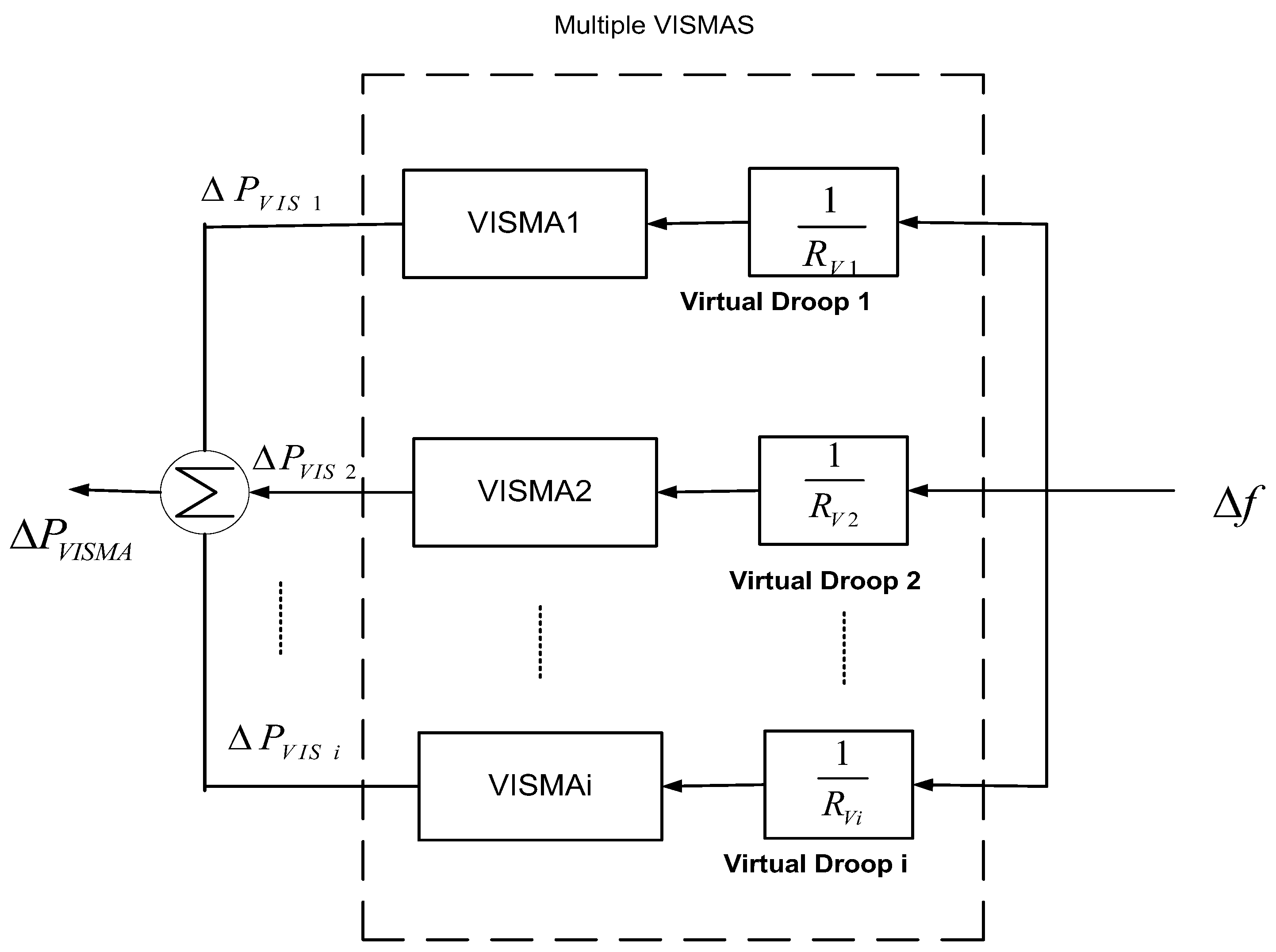
• With multiple VSIMA, frequency and grid stability is improved.
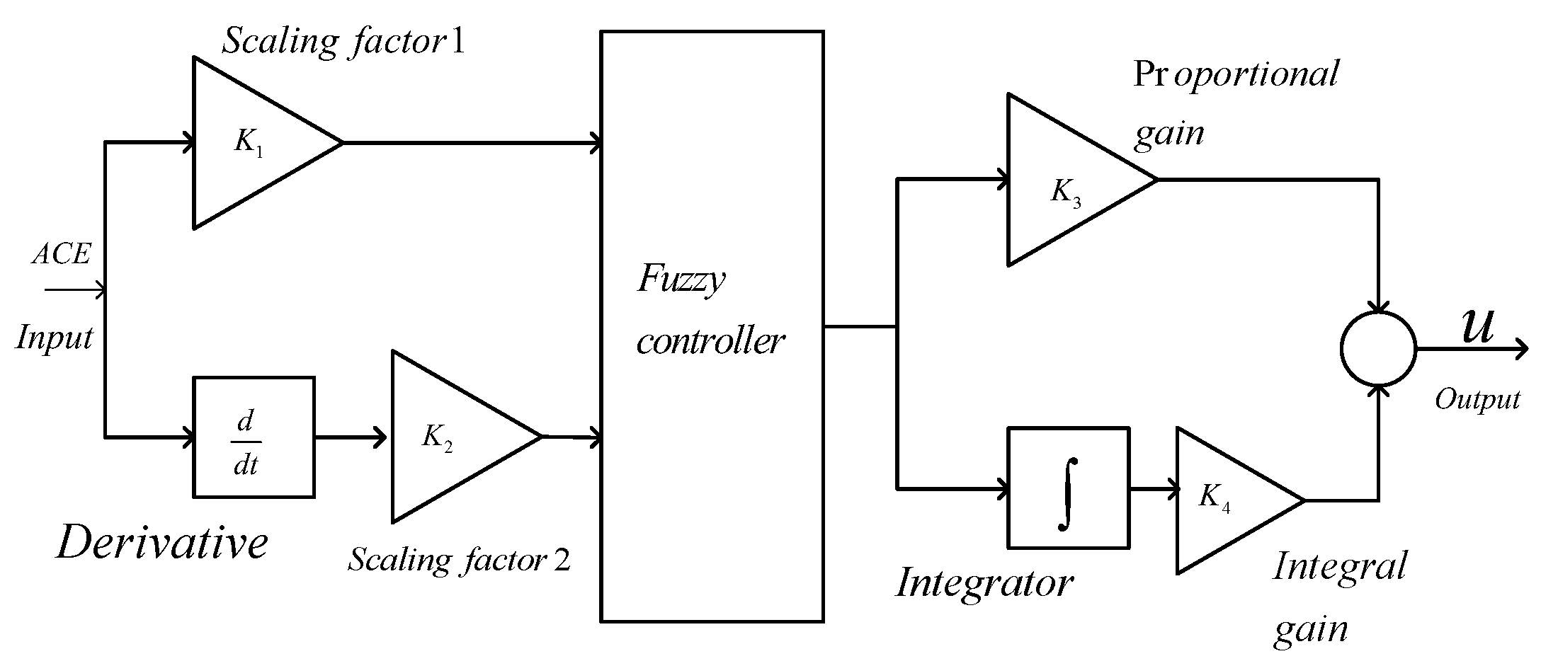
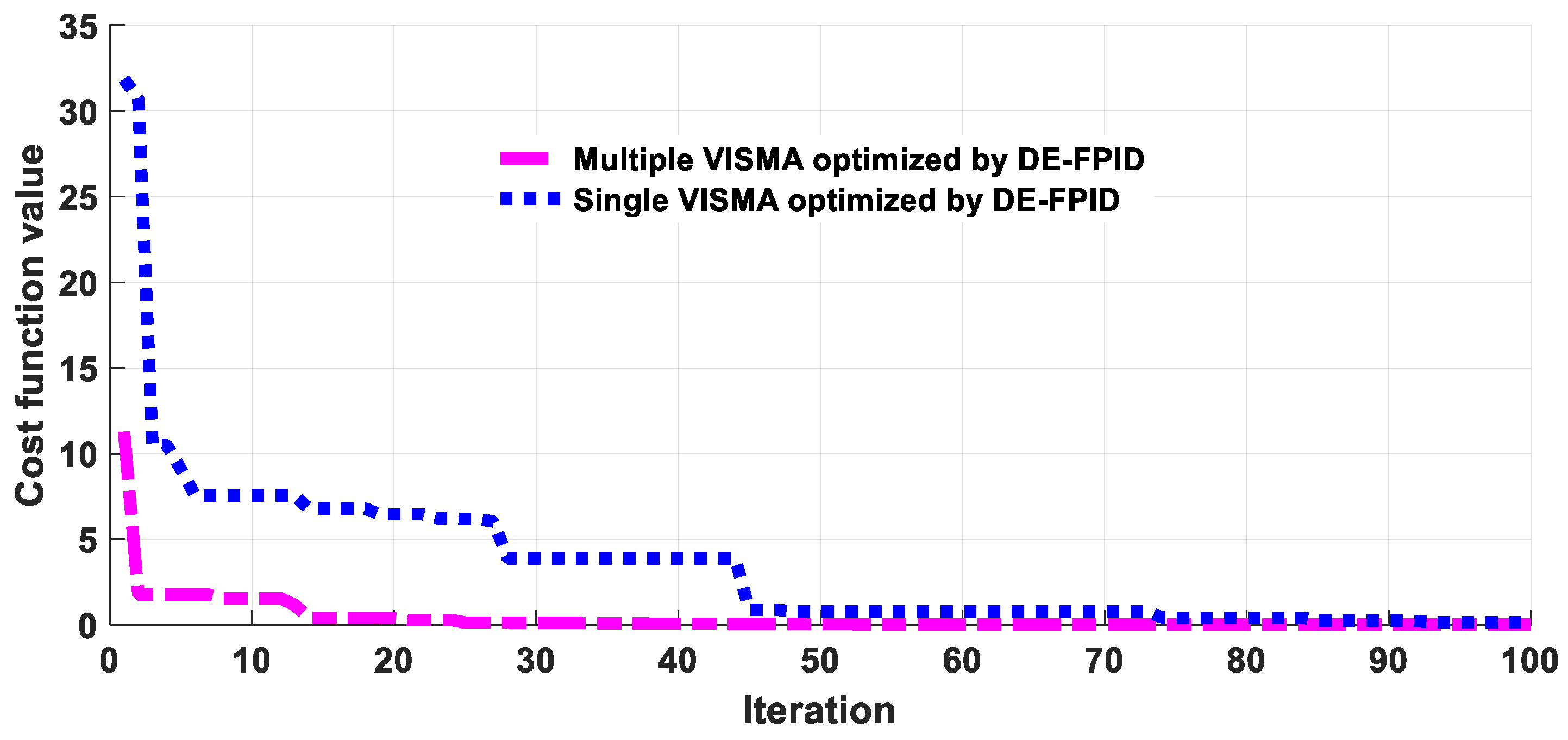
• With the proposed fuzzy proportional integral derivative (FPID) controllers optimized by DE using multiple VISMAs, the dynamic performance of the grid increases.
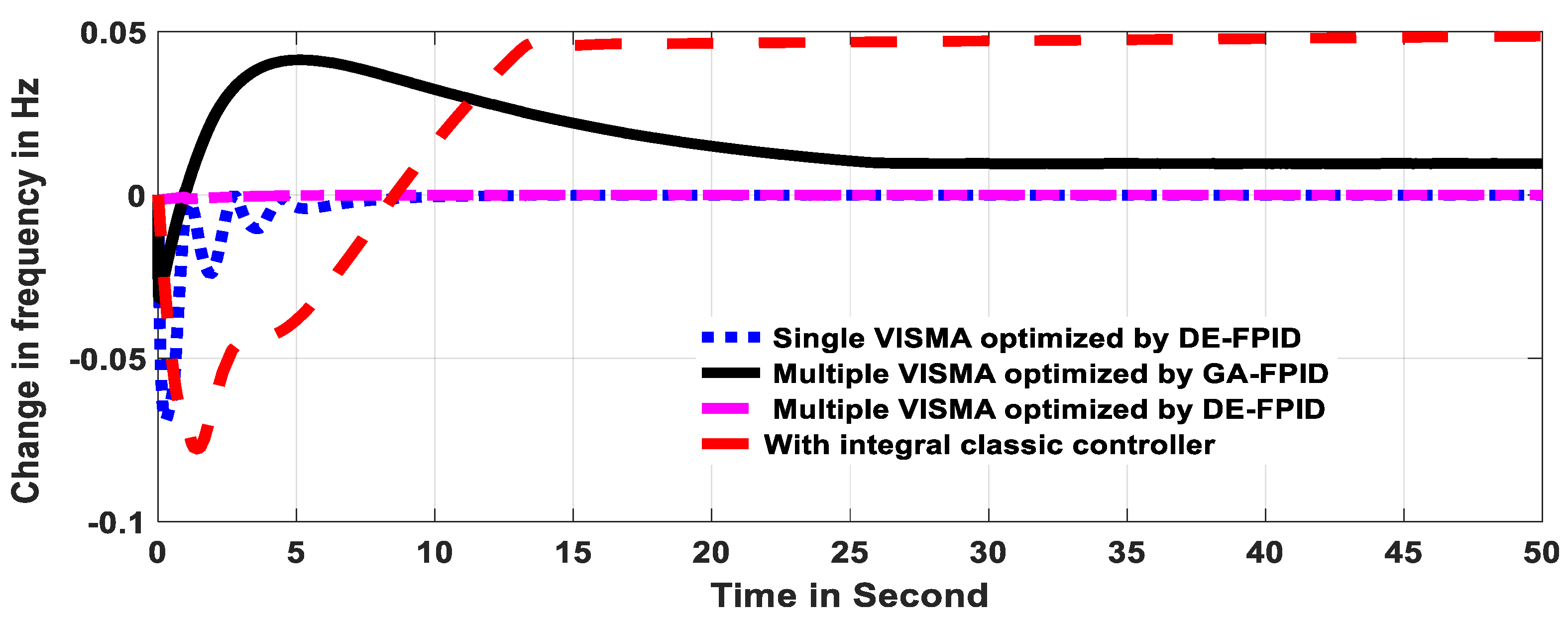
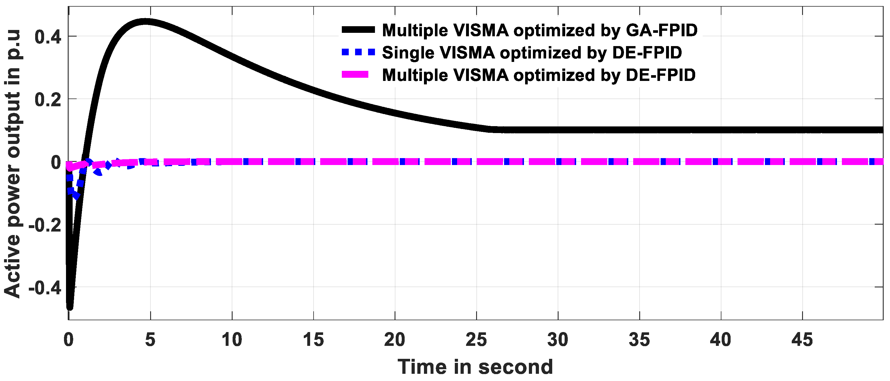
• The work showed better damping of grid oscillations in cases of multiple VISMAs with DE than in single VISMAs.
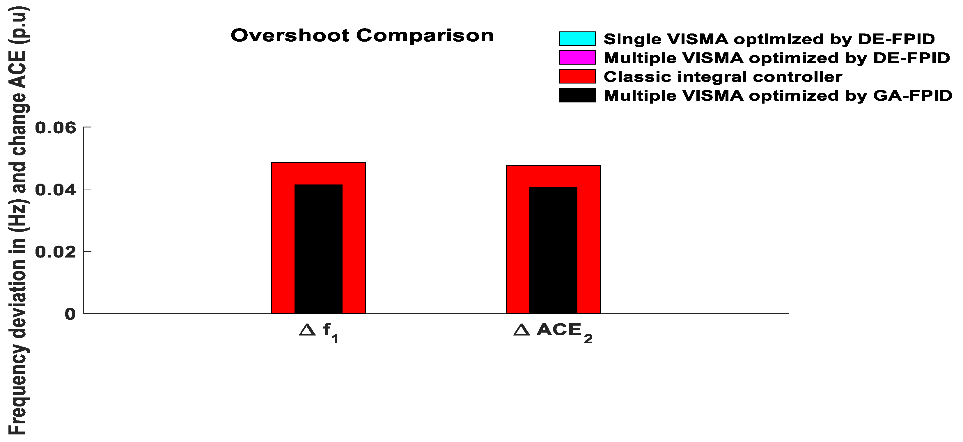
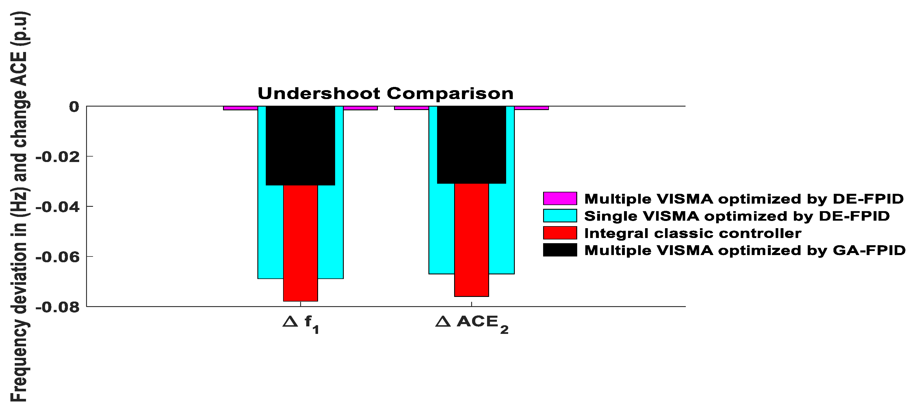
• Compared to the previous work in [8] using eigenvalue analysis, with the proposed method, the overshoot of change in frequency is reduced by 0.14999, and the undershoot of change in frequency is reduced by 0.1485.

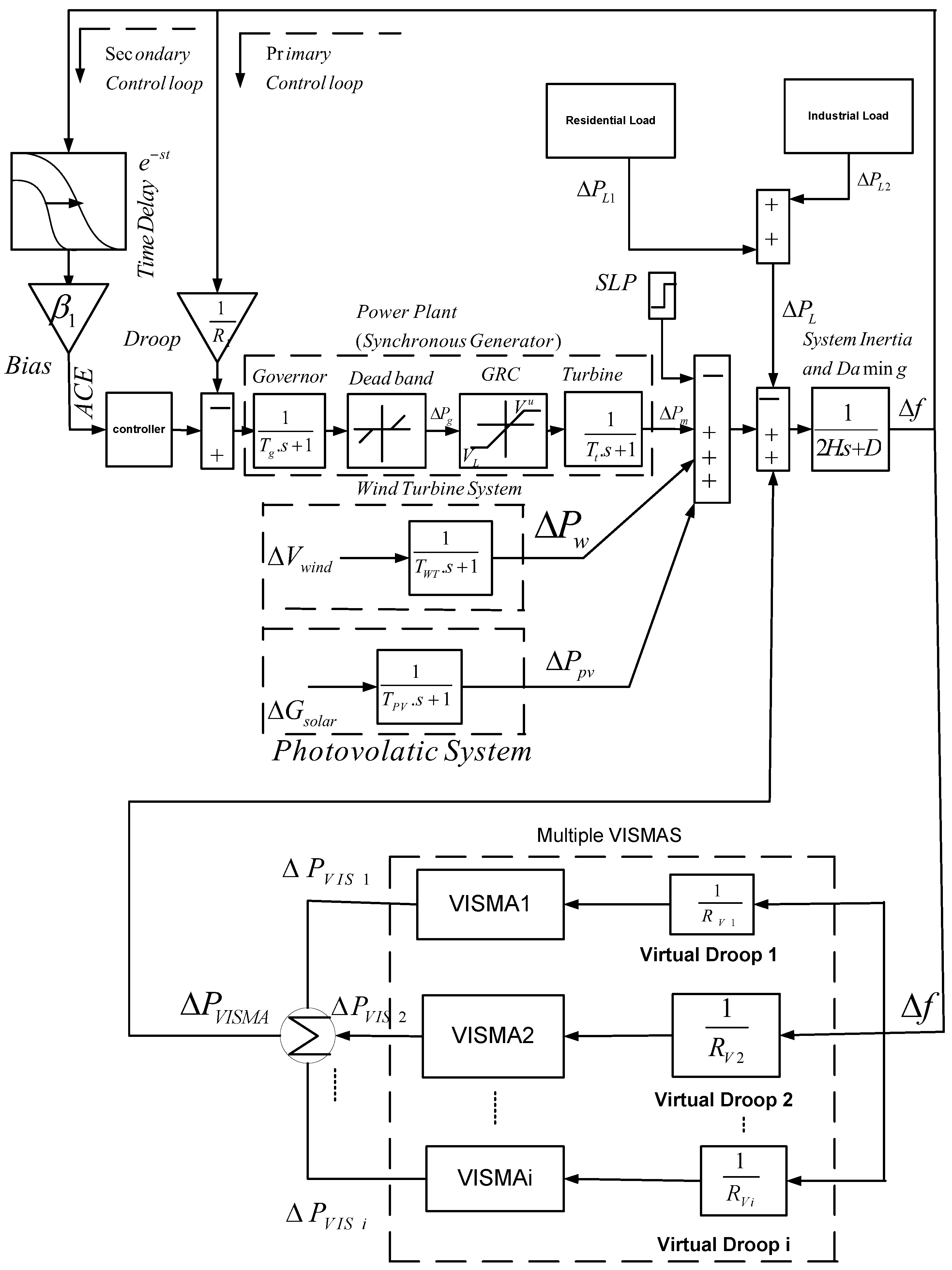
2. Materials and Methods

In this study, the grid in a power system integrating RESs, such as PV and wind, and loads, such as residential and industrial loads, are considered. To enhance the frequency and grid stability, single-VISMAs and multiple-VISMAs are optimized by optimization methods to control parameters such as frequency, ACE, and active power to make the grid stable, and the results have been compared. The parameters of RESs, such as solar, wind, and both industrial and residential loads, are optimized by DE and GA algorithms. The system models for the study of RES integration for single VISMAs and multiple VISMAs, respectively, are presented in Figure 1 and Figure 2, respectively. Similarly, small single-VISMA models for frequency analysis and multiple-VISMA models are depicted in Figure 3 and Figure 4, respectively. In the system modeling, to make the system more realistic, important physical limitations are considered, such as GRC, time delay, and dead band. Mathematical modeling for the analysis of the system under study is given in Equations (1)–(6) [8]. In the study, two strategies for controller optimization, (1) single VISMAs and (2) multiple VISMAs, with a system base of 15 MW, 6 MW of PV load, a 7 MW wind-turbine system, and 5 MW and 10 MW residential and industrial loads, respectively, have been considered. Moreover, to make the work more realistic, the integral classic controller is used to compare with the proposed intelligence controller.

2.1. Power System Equations

The synchronous generator shown in Figure 1, which consists of a governor, dead band, generation rate constraint (GRC), and turbine, are all involved in system control. For example, the governor will send a signal to the turbines if disturbance due to RES or load happens so that the generation tracks the system.

The gate opening and closing speed control systems in the GRC limiter block are represented by V_U and V_L for the upper and lower valves, respectively. And the change in the active power VISMAs of the turbine unit ∆P_m is given by Equation (1), where T_t and ∆P_g are the turbine time constant and change of speed governor control, respectively. The relationship between frequency in the secondary control loop and change in speed control is given in Equation (2).

$$\Delta P_m(s)=\frac{1}{1+s{T}_t}(\Delta P_g(s))$$

(1)

$$\Delta P_g(s)=\frac{1}{1+s{T}_g}(\Delta ACE(s)-\frac{1}{R}\Delta f(s)),$$

(2)

where, the droop constant R is involved in primary control, and the frequency change and governor time constant are given by ∆f and Tg, respectively. The change in area control error (∆ACE) measures the signal feedback coming from both primary and secondary control units. This frequency deviation is controlled in the secondary via the dynamic control of the fuzzy PID (FPID) controller and in the primary using the governor unit. Time delay (e^–st) is added to see its effect on communication delay during the performance-dynamic behavior of the secondary control. The secondary control for ACE is given in Equation (3).

$$\Delta ACE(s)=\frac{K_i\times \beta \times e^{-sT}\times \Delta f(s)}{s}$$

(3)

where K_i, which comprises K₁, K₂, K₃ and K₄, represents FPID controller-optimized gain values; T is the time delay constant; and β is the bias factor. The generated power ∆P_W depends on wind speed in wind turbine and is given by Equation (4)

$$\mathsf{\Delta }{P}_W\left(s\right)=\frac{1}{1+s{T}_{WT}}\mathsf{\Delta }{V}_{wind}\left(s\right)$$

(4)

where ∆V is the speed change for wind power. Solar irradiation is the basic means for generating electricity in PV; the power generated ∆P_PV in a PV system is given in Equation (5), where the solar constant is given by ∆G_solar.

$$\mathsf{\Delta }{P}_{PV}\left(s\right)=\frac{1}{1+s{T}_{PV}}\mathsf{\Delta }{G}_{solar}\left(s\right)$$

(5)

The frequency deviation in the small signal analysis after the disturbance due to (P_L) and RES power change (P_W, P_PV) is expressed in Equation (6), where H and D are the system inertia and damping coefficient constants, respectively, and ∆VISMAs is the (virtual) active power change [8].

$$\mathsf{\Delta }f\left(s\right)=\frac{1}{2H_s+D}\left(\mathsf{\Delta }{P}_m\right(s)+\mathsf{\Delta }{P}_W(s)+\mathsf{\Delta }{P}_{PV}(s)+\mathsf{\Delta }{P}_{VISMA}(s)-\mathsf{\Delta }{P}_L(s\left)\right)$$

(6)

In order to minimize the effect of noise and disturbances, the VISMAs model in Figure 3 comprises components such as inertia (Jvi), damping (D_vi), and low-pass filter block. In addition to this, to make the system more robust, time delay also used, which is shown in Figure 1. The time delay (e^−sT) in the system is included to perform the communication delays and dynamic behavior of filters. In addition, the time delay can also make the system robust. Figure 3 presents the small-signal stability analysis for frequency control, which consists of an inverter-based energy storage system (ESS) and the virtual rotor control action. To control the frequency, an inertia-emulation-based derivative technique is found to damp the disturbance [8].

2.2. Different Objective Function Analysis

$$ITAE={\displaystyle \underset{0}{\overset{t}{\int }}t.\left|AC{E}_i(t)\right|dt}$$

(7)

$$IAE={\displaystyle \underset{0}{\overset{t}{\int }}\left|AC{E}_i(t)\right|dt}$$

(8)

$$ITSE={\displaystyle \underset{0}{\overset{t}{\int }}t.AC{E}_i}{(t)}^{2}dt$$

(9)

$$ISE={\displaystyle \underset{0}{\overset{t}{\int }}AC{E}_i}{(t)}^{2}dt$$

(10)

Table 1. ITAE objective function time responses using DE + FPID controller.

Maeasured Variables	Rise Time	ST		Undershoot	Overshoot
Cahnge if f1	5.7426 × 10−5	8.3205		−0.0015	−1.4282 × 10−6
Change if ACE	5.0578 × 10−4	8.8344		−0.0014	−2.7761 × 10−6
Change in output P	4.8571 × 10−5	7.0645		−0.0214	−4.0462 × 10−5
The error in cost function			0.0219

,

Table 2. IAE objective function time responses using DE + FPID controller.

Maeasured Variables	Rise Time	ST		Undershoot	Overshoot
Cahnge if f1	7.9711 × 10−4	49.6977		−0.0840	0.0154
Change if ACE	0.0064	49.7039		−0.0823	0.0151
Change in output P	6.5204 × 10−4	48.5696		−1.2378	0.1834
The error in cost function			0.1662

,

Table 3. ISE objective function time responses using DE + FPID controller.

Maeasured Variables	Rise Time	ST		Undershoot	Overshoot
Cahnge if f1	1.4564	32.5382		0.0502	0.0739
Change if ACE	1.5336	26.1729		0.0504	0.0724
Change in output P	1.1245	49.7911		0.5393	0.7844
The error in cost function			0.0979

and

Table 4. ITSE objective function time responses using DE + FPID controller.

Maeasured Variables	Rise Time	ST		Undershoot	Overshoot
Cahnge if f1	0.3116	3.1474		0.0035	0.0077
Change if ACE	0.3209	3.6602		0.0037	0.0075
Change in output P	0.2473	23.6478		0.0379	0.0824
The error in cost function			0.0979

presents ITAE, IAE, ISE, and ITSE objectives of time response gain values, respectively. Compared to other objective functions, the ITAE controls the time response better. The tuning results for the system with ITAE settle much faster than other tuning methods. ITAE tuning also produces systems with a sluggish initial response. ITAE is chosen for this study because, when compared to ISE, ITSE, and IAE, it performs better in terms of reducing objective function error, undershoot, and overshoot.

2.3. Fuzzy Logic Controller

With a fuzzy logic controller, one can control the system under a wide range of operating conditions. For example, the truth values might lie between 0 and 1. Fuzzification, knowledge base, fuzzy inference, and defuzzification are the four types of steps in fuzzy logic, and each of them involves using rules in the input and output of system operation. [34]. The FPID controller model for this study is given in Figure 5.

Fuzzy theory was first proposed in 1965 by Professor Lotfi A. Zadeh. Unlike a fuzzy logic controller, whose true value lies between any two numbers [0, 1], the true value in a classical logic controller is either 0 or 1, and other very important features of fuzzy logic are that it is used for controlling non-linear systems in systems of higher order with a time delay. In this article, the FPID is designed using the fuzzy technique explained in [35,36].

Triangular membership functions are used in the work due to their advantages of fast response and low computational burden as well as their reduced undershoot and overshoot. The two inputs are a change in the error function (e) and derivative of the error function (de), and the output is (u). The rule-based output values are discussed in [33].

Table 5. The optimized fuzzy scaling factor parameters using DE + FPID.

Change in Error (e)	Derivation of Error (de)	Output (u)
−0.2  −0.2  −0.2  −0.1511	−0.02    −0.02     −0.02   −0.0160	−0.25  −0.25  −0.25  −0.1792
−0.1808  −0.1191  −0.0817	−0.0177    −0.0148    −0.0073	−0.2248  −0.1659  −0.0902
−0.1230  −0.0958  −0.0124	−0.0101   −0.0060     −0.0029	−0.1492 −0.1008 −0.0308
−0.0461     0    0.0631	−0.0054  0  0.0040	−0.06960    0.0418
0.0227  0.0363  0.1322	0.0015  0.0053   0.0110	0.0176  0.0799  0.1665
0.0970  0.1656  0.1894	0.0077  0.0121   0.0179	0.1171  0.2044  0.2095
0.1341  0.2  0.2  0.2	0.0162  0.02   0.02   0.02	0.1817  0.25  0.25  0.25

presents the optimized fuzzy scaling factor parameters using DE + FPID.

2.4. Optimization Problem

2.4.1. Genetic Algorithm

GA is a larger class in evolutionary algorithms, with the idea that the fittest will survive. GA, as part of artificial intelligence, employs genetic mutation and recombination. Initialization is the first step in the creation of a random population. A population size of 50 and total generation or iteration of 100 was used in all of the results presented here.

2.4.2. Differential Evolution

The following parameters are applied: iterations—100; population—50; decision variables boundaries—[0, 2]. From Darwinian evolutionary principles in DE, the individual at its fittest survival will leave a footprint for the next generation. It was proposed in 1995, and it has initialization, mutation, crossover, and selection and termination criteria [37].

Initialization

The initial population of a range [0, 2], which is the lower and upper limits of a predefined range, is randomly generated.

Mutation

With mutation, search quality will improve in DE.

Crossover

With the improvement in population diversity, in crossover, a new trial population is created.

Selection and Stop Criteria

In selection, an individual based on strong objective values is selected to form the next generation. A comparison is being made between the trial and current individuals in DE based on their objective values.

3. Result Analysis and Discussion

The power system shown in Figure 1 consists of an SG, wind-turbine system, photovoltaic system, residential load, industrial load, and VISMAs with two control strategies: single VISMAs and multiple VISMAs. The system control parameters are presented in

Table 6. System control parameters values.

S. No	Description	Symbol	Value
1	Speed-governor time constant (s),	Tg	0.07
2	Dead-band rate limit (Hz)		±0.018
3	Primary droop constant (Hz/p.u. MW),	R	2.4
4	Turbine time constant (s),	Tt	0.36
5	Upper valve/gate opening/closing speed (p.u.),	VU	+0.5
6	Lower valve/gate opening/closing speed (p.u.),	VL	−0.5
7	Frequency bias factor (p.u. MW Hz−1)	β	0.98
8	Time delay constant (s),	T	0.5
9	Virtual droop constant (s),	Rv	2.7
10	Virtual inertia constant (s),	Jv	1.6
11	Virtual damping constant (s),	Dv	1.3
12	Time constant of inverter-based ESS (s),	TEES	1.0
13	Maximum capacity of ESS (p.u. MW),	PESS_max	0.4
14.	Minimum capacity of ESS (p.u. MW),	PESS_min	−0.4
15	Time constant of wind turbine	TWT(s)	1.4
16	Time constant of solar system	TPV(s)	1.9
17	Inertia constant of the system (p.u. MW s),	H	0.083
18	Damping coefficient of the system (p.u. MW Hz−1),	D	0.016

. The system under study is considered to be 50 populations and 100 iterations. During simulation, the program runs for 108 h more than 10 times using the proposed FPID controller in the case of multiple VISMAs with DE optimization, with a simulation stopping time of 50 s. To identify the best controller for the system, the FPID controller is also optimized by the GA with multiple VISMAs, and the system ran with 50 populations and 100 iterations more than 10 times. The output power pattern in the presence of solar radiation and wind velocity is also depicted in Figure 6. Similarly, the load output pattern for residential and industrial loads is depicted in Figure 7.

Table 7. Optimum controller gains for multiple VISMAs optimized by DE-FPID.

Objective Function	Optimum Control Gains
ITAE	K1	K2	K3	K4	K5	K6	K7	K8
	0.0803	1.9631	0.1436	0.0100	0.0216	0.0107	0.0109	0.0115

shows the optimum controller gains for multiple VISMAs optimized by DE-FPID.

The simulation results presented in Figure 8, Figure 9 and Figure 10 show that, in the case of using a DE-optimized multiple VISMA, the better stability of the system is achieved for changes in frequency, changes in ACE, and changes in active power output of VISMAs than the systems optimized by a DE for single VISMAs and those optimized by a GA for multiple VISMAs. Moreover, Figure 11 depicts the convergence characteristic comparison between DE in multiple VISMAs and DE in single VISMAs, in which the proposed controller converges at a faster rate and at a lower cost function. The seven triangular membership function coordinate points of LN, MN, SN, Z, SP, MP, and LP are optimized during the simulation of multiple VISMAs using DE. In addition to this, the gain parameter variables K₁, K₂, K₃, and K₄ for FPID controllers, K5 and K6 for RESs of wind and solar, respectively, and K₇ and K₈ for residential and industrial loads, respectively, are optimized by DE in multiple VISMAs, by DE in single VISMAs, and by GA in multiple VISMAs, and the optimized values are presented in

Table 8. Optimum controller gains for single VISMAs optimized by DE-FPID.

Objective Function	Optimum Control Gains
ITAE	K1	K2	K3	K4	K5	K6	K7	K8
	1.3090	0.0308	1.2409	0.0355	0.0799	0.0762	0.0479	0.0983

,

Table 9. Optimum controller gains for multiple VISMAs optimized by GA-FPID.

Objective Function	Optimum Control Gains
ITAE	K1	K2	K3	K4	K5	K6	K7	K8
	0.6105	0.0382	0.0819	0.9189	0.6193	0.4476	0.1997	0.2960

and

Table 10. Integral controller value.

Integral controller

Integral Ki = 0.00068

, respectively.

The proposed controller has the lowest cost function, which is 0.0219 compared to the cost functions of single VISMAs optimized by DE and multiple VISMAs optimized by GA, and the comparison is presented in

Table 11. Comparison of ITAE error cost function values for different controllers.

Various Simulation Cases	ITAE Objective Function Value
Multiple VISMAs optimized by DE-FPID	0.0219
Single VISMAs optimized by DE-FPID	0.3268
Multiple VISMAs optimized by GA-FPID	15.3836
Classic integral controller	55.5338

. Measuring the transient response parameters in power systems is the most important factor and helps to analyze the rise time, setting time, undershoot, and overshoot. In this study, the optimized gains of these time response variables are optimized by using DE in multiple VISMAs, by using DE in single VISMAs, and by using GA in multiple VISMAs, and they are presented in

Table 12. Transient response of multiple VISMAs with DE.

Maeasured Variables	Rise Time	ST		Undershoot	Overshoot
Cahnge if f1	5.7426 × 10−5	8.3205		−0.0015	−1.4282 × 10−6
Change if ACE	5.0578 × 10−4	8.8344		−0.0014	−2.7761 × 10−6
Change in output P	4.8571 × 10−5	7.0645		−0.0214	−4.0462 × 10−5
The error in cost function			0.0219

,

Table 13. Transient response of single VISMAs with DE.

Maeasured Variables	Rise Time	ST		Undershoot	Overshoot
Cahnge if f1	6.9177 × 10−5	7.9905		−0.0689	−4.9628 × 10−6
Change if ACE	8.5616 × 10−4	8.5116		−0.0670	−4.0813 × 10−6
Change in output P	6.1766 × 10−5	7.1589		−0.1185	0.0036
The error in cost function			0.3268

and

Table 14. Transient response of multiple VISMAs with GA.

Maeasured Variables	Rise Time	ST		Undershoot	Overshoot
Cahnge if f1	0.3109	25.0302		−0.0315	0.0414
Change if ACE	0.3114	25.5142		−0.0308	0.0405
Change in output P	0.2616	24.4149		−0.04653	0.04468
The error in cost function			15.3836

, respectively, while the transient time response of the classical integral controller is presented in

Table 15. Transient response of classical integral controller.

Maeasured Variables	Rise Time	ST		Undershoot	Overshoot
Cahnge if f1	4.0327	15.8646		−0.0779	0.0486
Change if ACE	4.0358	16.2837		−0.0760	0.0476
The error in cost function			55.5338

. From the simulation results, the results have significantly improved by obtaining smaller rise time, undershoot, and overshoot when DE is used in optimizing multiple VISMAs as compared to the classical and other intelligent controllers. To make the comparison more convenient and clearer, the optimized parameter values of transient time response variables are compared as shown in Figure 12, Figure 13 and Figure 14 for rise time, overshoot, and undershoot, respectively.

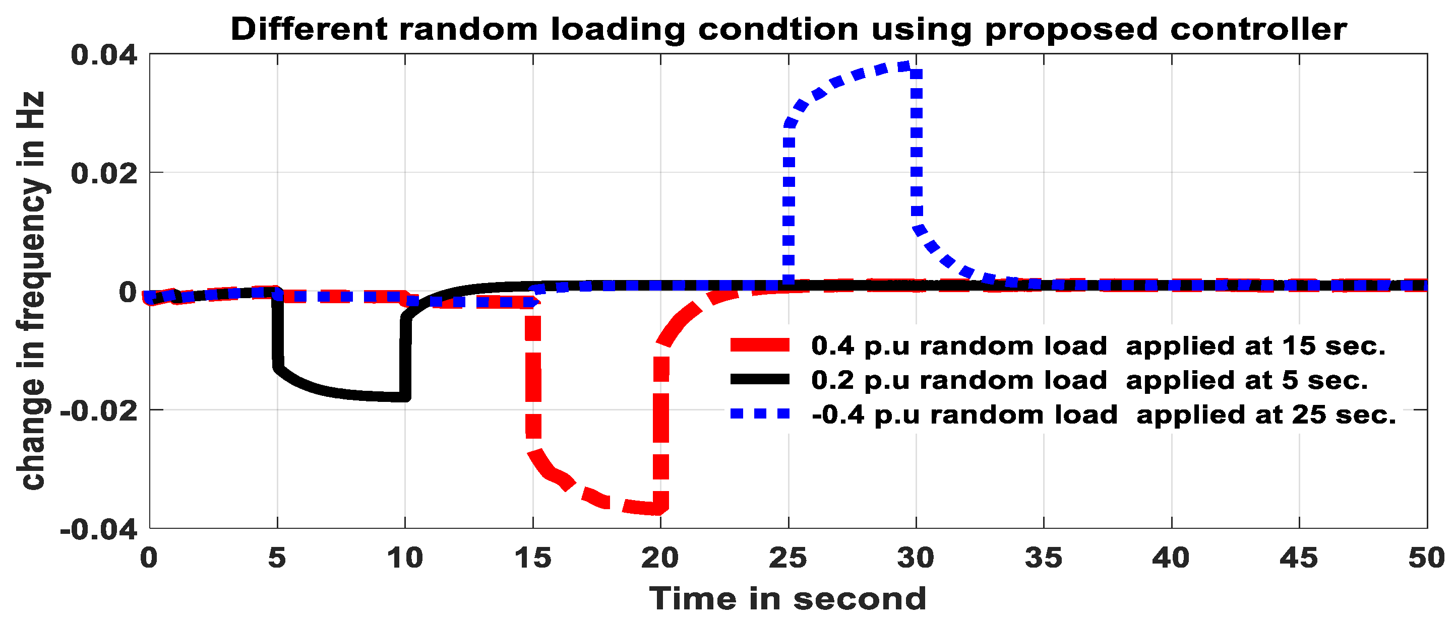
3.1. Results Analysis and Discussion on Random Load Change

Figure 15 is only depicted to show the random load pattern. Initially, a 0.01 load disturbance is considered for normal optimization during the simulation of the system, while to check the robustness of the proposed controller, a random load of ±0.2 p.u is added to the system, and further, when the random load is also increased to ±0.4 p.u, the proposed controller withstands the disturbances, and the simulation result is also shown in Figure 16. As observed in Figure 16, when the load drops to −0.4, the frequency increases, while when the load increases to 0.4, the frequency drops. However, the proposed controller stabilizes the system more quickly with a smaller random load as compared to a bigger random load.

3.2. Discussion on Result Comparison with Classic Control and Other Studies

For comparison reasons, the classic integral controller was used in this study and compared with the intelligent FPID controller optimized by the evolutionary techniques. In the result analysis, it is shown in Figure 8 and Figure 9 that, compared to the classic integral controller with the intelligent controller of the proposed multiple VISMAs with DE, smaller settling time, undershoot, overshoot, and rise time have been achieved. Similarly, the ITAE error cost function of multiple VISMAs with DE is 0.0219, which is much smaller than the classical integral controller, which is 55.5338, as shown in Table 11. The results of time response overshoot and undershoot frequency measurement for the proposed method in multiple VISMAs using the DE optimization method in the presence of an FPID controller and the previous published paper using eigenvalue time domain analysis in [8] have been compared in

Table 16. Comparison between the previous result and the proposed method.

Frequency Response in (Hz) in the Previous Published Paper Using Eigenvalue Time Domain Analysis [8]		Frequency Response in (Hz) Using the Proposed FPID Optimized Using DE Technique
undershoot	overshoot	undershoot	overshoot
−0.15	0.15	−0.0015	−1.4282 × 10−6

, and it reveals that with the proposed controller, significant improvements were observed in terms of results.

4. Conclusions

This article is basically concerned with enhancing the frequency stability of the system by a multiple VISMA technique. In this work, single and multiple VISMAs optimized by DE are compared with the multiple VISMAs optimized by the GA. The dynamic simulation output of change in frequency, change in ACE, and change in active power output are compared and reveal that with multiple VISMAs optimized by DE better results are achieved. The error in the objective function from the minimum threshold set values are much higher in a single VISMA system than in a multiple VISMA system, which are 0.3268 and 0.0219, respectively. This implies that by using multiple VISMAs in the proposed controller, the error is reduced by approximately 13.9 times. It is also shown that compared to the previous work performed by eigenvalue analysis in [8], by using the proposed controller, overshoot of change in frequency is reduced by 0.14999, which in percentage is improved by 99.99%; similarly, undershoot of change in frequency is reduced by 0.1485 and the improved percentage is 99%; and the comparison is also presented in Table 16. Moreover, compared to the classical integral, for single VISMAs with DE and multiple VISMAs using the GA and multiple VISMAs optimized by DE, a smaller rise time, reduced undershoot, and reduced overshoot are achieved for changes in frequency and changes in ACE. To examine the robust operation of the system under the proposed controller, the system was run under a wide range of disturbances and uncertainties using random load perturbation of ±20%, in which the proposed controller retains the system frequency by reducing or damping the system oscillation.

References

1. Cheema, K.M.; Chaudhary, N.I.; Tahir, M.F.; Mehmood, K.; Mudassir, M.; Kamran, M.; Milyani, A.H.; Elbarbary, Z.S. Virtual synchronous generator: Modifications, stability assessment and future applications. Energy Rep. 2022, 8, 1704–1717. [Google Scholar] [CrossRef]
2. Bevrani, H.; Ise, T.; Miura, Y. Virtual synchronous generators: A survey and new perspectives. Int. J. Electr. Power Energy Syst. 2014, 54, 244–254. [Google Scholar] [CrossRef]
3. Zhong, Q.C. Virtual synchronous machines: A unified interface for smart grid integration. IEEE Power Electron. Mag. 2016, 3, 18–27. [Google Scholar] [CrossRef]
4. Petti, J. Virtual Synchronous Machine Phase Synchronization. Ph.D. Thesis, University of Pittsburgh, Pittsburgh, PA, USA, 2018. [Google Scholar]
5. Gaur, P.; Singh, S. Investigations on issues in microgrids. J. Clean Energy Technol. 2017, 5, 47–51. [Google Scholar] [CrossRef]
6. Martins, F.J.N. Virtual Synchronous Machine. TecnicoLisboa, ULisboa, 2016. Available online: https://fenix.tecnico.ulisboa.pt/downloadFile/395145918861/paper.pdf (accessed on 1 March 2020).
7. Li, L.; Li, H.; Tseng, M.L.; Feng, H.; Chiu, A.S. Renewable energy system on frequency stability control strategy using virtual synchronous generator. Symmetry 2020, 12, 1697. [Google Scholar] [CrossRef]
8. Kerdphol, T.; Rahman, F.S.; Watanabe, M.; Mitani, Y.; Hongesombut, K.; Phunpeng, V.; Ngamroo, I.; Turschner, D. Small-signal analysis of multiple virtual synchronous machines to enhance frequency stability of grid-connected high renewables. IET Gener. Transm. Distrib. 2021, 15, 1273–1289. [Google Scholar] [CrossRef]
9. D’Arco, S.; Suul, J.A.; Fosso, O.B. A Virtual Synchronous Machine implementation for distributed control of power converters in SmartGrids. Electr. Power Syst. Res. 2015, 122, 180–197. [Google Scholar] [CrossRef]
10. Yang, L.; Ma, J.; Wang, S.; Liu, T.; Wu, Z.; Wang, R.; Tang, L. The strategy of active grid frequency support for virtual synchronous generator. Electronics 2021, 10, 1131. [Google Scholar] [CrossRef]
11. Chen, Y.; Hesse, R.; Turschner, D.; Beck, H.P. Dynamic properties of the virtual synchronous machine (VISMA). Proc. Icrepq 2011, 11, 755–759. [Google Scholar] [CrossRef]
12. Tayyebi, A.; Groß, D.; Anta, A.; Kupzog, F.; Dörfler, F. Frequency stability of synchronous machines and grid-forming power converters. IEEE J. Emerg. Sel. Top. Power Electron. 2020, 8, 1004–1018. [Google Scholar] [CrossRef]
13. Zhong, C.; Li, H.; Zhou, Y.; Lv, Y.; Chen, J.; Li, Y. Virtual synchronous generator of PV generation without energy storage for frequency support in autonomous microgrid. Int. J. Electr. Power Energy Syst. 2022, 134, 107343. [Google Scholar] [CrossRef]
14. Zhang, G.; Yang, J.; Wang, H.; Cui, J. Presynchronous grid-connection strategy of virtual synchronous generator based on virtual impedance. Math. Probl. Eng. 2020, 2020, 3690564. [Google Scholar] [CrossRef]
15. Miao, H.; Mei, F.; Yang, Y.; Chen, H.; Zheng, J. A comprehensive VSM control strategy designed for unbalanced grids. Energies 2019, 12, 1169. [Google Scholar] [CrossRef]
16. Adefarati, T.; Bansal, R.C. Integration of renewable distributed generators into the distribution system: A review. IET Renew. Power Gener. 2016, 10, 873–884. [Google Scholar] [CrossRef]
17. Tamrakar, U.; Shrestha, D.; Maharjan, M.; Bhattarai, B.P.; Hansen, T.M.; Tonkoski, R. Virtual inertia: Current trends and future directions. Appl. Sci. 2017, 7, 654. [Google Scholar] [CrossRef]
18. Abuagreb, M.; Allehyani, M.F.; Johnson, B.K. Overview of Virtual Synchronous Generators: Existing Projects, Challenges, and Future Trends. Electronics 2022, 11, 2843. [Google Scholar] [CrossRef]
19. Magdy, G.; Bakeer, A.; Nour, M.; Petlenkov, E. A new virtual synchronous generator design based on the SMES system for frequency stability of low-inertia power grids. Energies 2020, 13, 5641. [Google Scholar] [CrossRef]
20. Sang, W.; Guo, W.; Dai, S.; Tian, C.; Yu, S.; Teng, Y. Virtual Synchronous Generator, a Comprehensive Overview. Energies 2022, 15, 6148. [Google Scholar] [CrossRef]
21. Li, C.; Yang, Y.; Cao, Y.; Wang, L.; Blaabjerg, F. Frequency and voltage stability analysis of grid-forming virtual synchronous generator attached to weak grid. IEEE J. Emerg. Sel. Top. Power Electron. 2020, 10, 2662–2671. [Google Scholar] [CrossRef]
22. Gunasekara, R.; Muthumuni, D.; Filizadeh, S.; Kho, D.; Marshall, B.; Ponnalagan, B.; Adeuyi, O.D. A novel virtual synchronous machine implementation and verification of its effectiveness to mitigate renewable generation connection issues at weak transmission grid locations. IET Renew. Power Gener. 2023, 17, 2436–2457. [Google Scholar] [CrossRef]
23. Lu, L.; Cutululis, N.A. Virtual synchronous machine control for wind turbines: A review. In Journal of Physics: Conference Series; IOP Publishing: Bristol, UK, 2019; Volume 1356, p. 012028. [Google Scholar]
24. Dewenter, T.; Heins, W.; Werther, B.; Hartmann, A.K.; Bohn, C.; Beck, H.P. Parameter Optimisation of a Virtual Synchronous Machine in a Microgrid. arXiv 2016, arXiv:1606.07357. [Google Scholar]
25. Wen, T.; Zhu, D.; Zou, X.; Jiang, B.; Peng, L.; Kang, Y. Power coupling mechanism analysis and improved decoupling control for virtual synchronous generator. IEEE Trans. Power Electron. 2020, 36, 3028–3041. [Google Scholar] [CrossRef]
26. Shi, R.; Zhang, X.; Hu, C.; Xu, H.; Gu, J.; Cao, W. Self-tuning virtual synchronous generator control for improving frequency stability in autonomous photovoltaic-diesel microgrids. J. Mod. Power Syst. Clean Energy 2018, 6, 482–494. [Google Scholar] [CrossRef]
27. Feleke, S.; Satish, R.; Pydi, B.; Anteneh, D.; Abdelaziz, A.Y.; El-Shahat, A. Damping of Frequency and Power System Oscillations with DFIG Wind Turbine and DE Optimization. Sustainability 2023, 15, 4751. [Google Scholar] [CrossRef]
28. Rahman, F.S.; Kerdphol, T.; Watanabe, M.; Mitani, Y. Optimization of virtual inertia considering system frequency protection scheme. Electr. Power Syst. Res. 2019, 170, 294–302. [Google Scholar] [CrossRef]
29. Liu, D. Cluster control for EVS participating in grid frequency regulation by using virtual synchronous machine with optimized parameters. Appl. Sci. 2019, 9, 1924. [Google Scholar] [CrossRef]
30. Niu, S.; Qu, L.; Lin, H.C.; Fang, W. Effective virtual inertia control using inverter optimization method in renewable energy generation. Energy Explor. Exploit. 2021, 39, 2103–2125. [Google Scholar] [CrossRef]
31. Feleke, S.; Satish, R.; Tatek, W.; Abdelaziz, A.Y.; El-Shahat, A. DE-Algorithm-Optimized Fuzzy-PID Controller for AGC of Integrated Multi Area Power System with HVDC Link. Energies 2022, 15, 6174. [Google Scholar] [CrossRef]
32. Feleke, S.; Pydi, B.; Satish, R.; Anteneh, D.; AboRas, K.M.; Kotb, H.; Alharbi, M.; Abuagreb, M. DE-Based Design of an Intelligent and Conventional Hybrid Control System with IPFC for AGC of Interconnected Power System. Sustainability 2023, 15, 5625. [Google Scholar] [CrossRef]
33. Trillas, E.; Lotfi, A. Zadeh: On the man and his work. ScientiaIranica 2011, 18, 574–579. [Google Scholar]
34. Justice, A.V.; Kathyaini, C. Controlling of nonlinear systems by using fuzzy logic controller. Int. Res. J. Eng. Technol. 2015, 2, 648–656. [Google Scholar]
35. Pothiya, S.; Ngamroo, I.; Runggeratigul, S.; Tantaswadi, P. Design of optimal fuzzy logic based PI controller using multiple tabu search algorithm for load frequency control. Int. J. Control Autom. Syst. 2006, 4, 155–164. [Google Scholar]
36. Storn, R.; Price, K. Differential evolution—A simple and efficient heuristic for global optimization over continuous spaces. J. Glob. Optim. 1997, 11, 341–359. [Google Scholar] [CrossRef]
37. Rehman, H.U.; Yan, X.; Abdelbaky, M.A.; Jan, M.U.; Iqbal, S. An advanced virtual synchronous generator control technique for frequency regulation of grid-connected PV system. Int. J. Electr. Power Energy Syst. 2021, 125, 106440. [Google Scholar] [CrossRef]
Figure 1. RES integration in single VISMA.
Sustainability 15 13892 g001
Figure 2. RES integration in multiple VISMAs.
Sustainability 15 13892 g002
Figure 3. Small-signal VISMA models for frequency analysis.
Sustainability 15 13892 g003
Figure 4. Multiple-VISMA model for small signal dynamic analysis.
Sustainability 15 13892 g004
Figure 5. FPID controller model [33].
Sustainability 15 13892 g005
Figure 6. Power from RESs.
Sustainability 15 13892 g006
Figure 7. Residential and industrial load demand.
Sustainability 15 13892 g007
Figure 8. Change in frequency output comparisons in case of single and multiple VISMAs.
Sustainability 15 13892 g008
Figure 9. Change in ACE output comparisons in case of single and multiple VISMAs.
Sustainability 15 13892 g009
Figure 10. Change in active power output comparisons in the case of single and multiple VISMAs.
Sustainability 15 13892 g010
Figure 11. Comparisons of convergence characteristics in the case of single and multiple VISMAs.
Sustainability 15 13892 g011
Figure 12. Rise time comparison for change in frequency and change in area control error.
Sustainability 15 13892 g012
Figure 13. Overshoot comparison for change in frequency and change in area control error.
Sustainability 15 13892 g013
Figure 14. Undershoot comparison for change in frequency and change in area control error.
Sustainability 15 13892 g014
Figure 15. Random load change pattern ranging from [−0.2 to 0.2].
Sustainability 15 13892 g015
Figure 16. Change in frequency output in case of different random load applications using the proposed controller.
Sustainability 15 13892 g016