A Differentiated Dynamic Reactive Power Compensation Scheme for the Suppression of Transient Voltage Dips in Distribution Systems

Abstract

At present, with the construction of new power systems, the uncertainty of the system is increasing and the transient voltage stability of the power grid is becoming more and more complicated. For this reason, this paper proposes a differentiated dynamic reactive power compensation configuration method for suppressing transient voltage dip instability. The method first establishes a dynamic reactive power device configuration indicator system based on multiple-two-element notation, and then establishes a differentiated dynamic reactive power compensation device configuration model based on the node instability risk characteristics. The model takes the investment cost and suppression effect as the optimization objectives, and flexibly adjusts the optimization weights of its cost and suppression effect according to the high or low risk of the transient voltage instability of the compensation node, so as to realize the differentiated dynamic reactive power compensation. Compared with traditional compensation methods, differentiated compensation can significantly improve the economic benefits of reactive power compensation configuration. Finally, taking the IEEE39 node test system as an example, the improved TLBO algorithm is used to solve the model. The cost of differentiated compensation is reduced by 22.13%, with a similar suppression effect, which verifies the validity of the method proposed in this paper.

1. Introduction

The rapid development of the modern power network, with the gradual construction of a new power system, the DC transmission system, the widespread application of electronic power equipment, new energy access, and induction motor loads, has created a number of serious problems. Notably, it has led to the weakening of a growing proportion of the power system’s voltage regulation capacity and an increase in the risk of transient voltage instability; specifically, it has caused a decline in the abilities of transient reactive power support.

A dynamic reactive power compensation device can react quickly when a grid fault occurs, provide a large amount of reactive power, and inhibit transient voltage dips, thus preventing system transient voltage instability [1]. Dynamic reactive power compensation technology is an important and effective means of improving the reliability of power system operations and increasing the stability margin. Compared with traditional static reactive power compensation devices, such as switched capacitor banks or reactor banks, dynamic reactive power compensation devices have stronger transient reactive power output capabilities, faster response speeds, and increased capacity, but also higher costs. So-called static compensation means that the compensation capacitor does not follow the fluctuations of reactive power and real-time tracking and cutting, and the general delay is more than 40 s. Dynamic compensation involves the compensation capacitor casting in order to follow the load of reactive power changes; the process, from the detection of the signal to the execution of the casting, is completed within 10–20 ms. Reasonable planning of the location, the selection of the device types according to different device characteristics, and the determination of the installation capacity are necessary prerequisites for dynamic reactive power compensation devices, ensuring that the reactive power compensation effect is fully realized [2].

The disadvantage of dynamic reactive power compensation is that it is expensive, with high configuration and maintenance costs, and it is not practical to universally configure it in practical engineering applications. Therefore, it is necessary to consider the reasonable arrangement of the distribution points and the capacity of dynamic reactive power compensation devices during the planning stage [3]. At present, the research on the optimal configuration of dynamic reactive power compensation devices mainly focuses on the selection of reasonable installation locations, and the methods used are generally methods of analyzing static voltage stability, such as the pilot node method, the U–Q curve method, and the participation factor method [4]. However, the main purpose of the dynamic reactive power compensation device should be to improve the transient voltage stability of the system, rather than to improve the static voltage stability margin, so it is more appropriate to use the analytical method of transient voltage stability to determine the installation location and capacity of the dynamic reactive power compensation device. The study reported in [5] determines the transient voltage stability by comparing the magnitude of the motor slip before and after the fault and the magnitude of electromagnetic torque and mechanical torque when the voltage reaches its extreme value. However, comparing the slip or torque alone does not accurately reflect whether the motor is unstable, and it is challenging to use in engineering practice. Another criterion involves judging the transient voltage stability according to the time when the voltage is lower than a certain threshold in the transient process, and [6] stipulates that, during the transient process, the load bus voltage can be restored to more than 0.80 p.u. within 10 s after the fault. Another study [7] stipulates that the time for which the pivot point bus voltage remains below 0.75 p.u. is not more than 1 s, and that the pivot point bus voltage at 220 KV and above is not less than 0.9 p.u. after the end of the transient process. The authors of [8] define this criterion as transient voltage drop acceptability, and this kind of criterion can usually only be used to qualitatively judge the stability of transient voltage, without considering the influence of the voltage drop, and it cannot quantitatively analyze the voltage stability.

In addition, the research on the capacity configuration of dynamic reactive power compensation devices is still relatively sparse and lacks a differentiated analysis of the characteristics of the compensation nodes, which can easily lead to the over-compensation of the nodes and make it difficult to improve the device’s economy. The authors of [9] used the mean–variance mapping algorithm to optimize the STATCOM capacity of compensation node configuration using the short-circuit ratio as a constraint. Elsewhere, [10] regarded the capacity of each dynamic reactive power compensation device as a fixed value, and calculated the compensation effect indexes of all the candidate deployment locations by using the cyclic deployment method to determine the compensation capacity. However, this method does not take into account the characteristics of the compensation nodes and cannot realize the fine planning of the compensation capacity.

Based on the above research and the existing problems in the field, this paper proposes a differentiated dynamic reactive power compensation configuration method based on transient voltage assessment indexes. It is based on multiple-two-element notation for suppressing transient voltage dips, differentiating compensation according to the characteristics of the device type, and flexibly considering the weight of the optimization objective to minimize the configuration cost and improve the economics. Section 2 of this paper analyzes the mechanism of voltage multi-binary tables, proposes the safety margin index of transient voltage dips for buses and systems, determines the set of the most serious fault scenarios, and divides the risk regions of transient voltage instability of different grades; Section 3 establishes the model of a node-differentiated dynamic reactive power compensation device according to the division of the risk regions of instability, reasonably adjusts the optimization weights of nodes with different risk regions, and makes use of the improved multi-objective genetic algorithm in the IEEE39 node system using PSD-BPA and MATLAB joint simulation of the proposed method in Section 2 and Section 3 for calculation and model solving, which verifies the effectiveness of the proposed method.

The contributions are as follows:

(1)

The configuration method employs transient voltage stability analysis to determine the ideal installation locations and capacities for dynamic reactive power compensation devices. It appropriately expands the referenced multi-binary table indexes and introduces a specialized index system for optimizing dynamic reactive power compensation device configurations. Furthermore, it establishes a model for differentiated compensation strategies, with enhancements made to the TLBO algorithm for effective model solving.

(2)

Within this configuration method, a differentiated compensation component is introduced, allowing for flexible adjustments based on the weights of optimal configuration objectives. These adjustments are made considering the varying levels of instability risk across different system regions and the unique characteristics of the reactive power compensation device types. In comparison with traditional methods, even with similar reactive power compensation results, this approach has the potential to reduce configuration costs and enhance overall economic efficiency.

2. Dynamic Reactive Device Configuration Index System Based on Multiple-Two-Element Notation

2.1. Multiple-Two-Element Notation Criterion

Currently, the international practice in assessing system transient voltage instability typically relies on engineering empirical criteria. This approach involves a rough determination of the system’s voltage stability by observing the depth of voltage drop and the corresponding duration at each busbar following a fault disturbance. It is important to note that this practical criterion can only ascertain whether the voltage is stable or not, without providing information about the extent of stability [11].

In contrast, the multi-binary tables criterion offers a more precise method for evaluating transient voltage stability. It achieves this by integrating the transient voltage response curve and quantitatively analyzing predetermined threshold levels for both the depth and duration of voltage deviations. Among various transient voltage quantization methods, the transient voltage stability margin index based on the multiple-two-element notation criterion stands out, as it provides a significant advantage. It allows for a quantitative assessment of the improvement achieved with dynamic reactive power compensation on transient voltage [12].

The fundamental concept of the multiple-two-element notation criterion involves configuring n voltage two-element notations {[V_cr¹, T_cr¹], [V_cr², T_cr²], …, [V_crⁿ, T_crⁿ]} within the electrical power system to assess transient voltage stability. For any individual voltage two-element notation, it is essential to ensure that the voltage at a bus remains below a predefined threshold for a maximum specified duration. When these conditions are met, the transient voltage at the bus is considered stable; otherwise, it is deemed destabilized. Following the principle of integrating voltage perturbation trajectories and assigning varying weights to different levels of voltage dips, this criterion refines the impact of voltage dip levels on system stability, as illustrated in Figure 1.

For bus i, define the safety margin for transient voltage dips as follows:

$${\eta }_{V_i}=1-{\displaystyle \sum _{k=1}^{n-1}{K}_k}{\displaystyle {\int }_{t_k}^{t_{k+1}}\left[V_{i\mathrm{N}}-V_i(t)\right]}\mathrm{d}t-K_n{\displaystyle {\int }_{t_n}^{t_n^{\prime }}[V_{i\mathrm{N}}-} V_i(t)]\mathrm{d}t-{\displaystyle \sum _{k=1}^{n-1}{K}_k}{\displaystyle {\int }_{t_{k+1}^{\prime }}^{t_k^{\prime }}\left[V_{i\mathrm{N}}-V_i(t)\right]}\mathrm{d}t$$

(1)

t_k and t_k′ represent the system transient process of bus i transient voltage V_i(t) twice through the V_cr^k moment; K_k corresponds to the kth two-element notation [V_cr^k, T_cr^k] weight coefficients; V_iN is the rated voltage of the bus i, the value of which can be set according to relevant standards, where buses need to meet the (0.75 p.u.,1 s) and (0.8 p.u.,10 s) standard requirements [13]. When η_Vi > 0, the system transient voltage is stable; conversely, when η_Vi < 0, the transient voltage is unstable.

In the dynamic process, when the system state is critically stable, it satisfies η_{Vi =} 0. The weight coefficients are solved as follows.

$$\{\begin{array}{l}{K}_1\left(V_{\mathrm{iN}}-V_{\mathrm{cr}}{}^1\right)T_{\mathrm{cr}}{}^1=1\\ K_1\left(V_{\mathrm{iN}}-V_{\mathrm{cr}}{}^1\right)T_{\mathrm{cr}}{}^2+K_2\left(V_{\mathrm{iN}}-V_{\mathrm{cr}}{}^2\right)T_{\mathrm{cr}}{}^2=1\\ ⋮\\ K_1\left(V_{\mathrm{iN}}-V_{\mathrm{cr}}{}^1\right)T_{\mathrm{cr}}{}^2+K_2\left(V_{\mathrm{iN}}-V_{\mathrm{cr}}{}^2\right)T_{\mathrm{cr}}{}^{\mathrm{n}}+\cdots +K_n\left(V_{\mathrm{iN}}-V_{\mathrm{cr}}{}^n\right)T_{\mathrm{cr}}{}^n=1\end{array}$$

(2)

For Equation (2), the deeper the voltage dip, the shorter its maximum acceptable duration. Generally, having V_crⁱ < V_cr^j when T_crⁱ < T_cr^j results in larger corresponding weighting coefficients; conversely, the shallower the dip, the smaller the corresponding weighting coefficients.

2.2. Indicator of Safety Margin for Integrated Transient Voltage Dips of the System

The selection of the optimal node for reactive power compensation should be able to take into account the improvement effect of the configured reactive power compensation device on the overall voltage stability of the system. Based on the transient voltage dip safety margin index of the node in Equation (1), the comprehensive transient voltage dip safety margin index Γ of the regional system is proposed, and its calculation method is as follows:

$$\Gamma ={\displaystyle \sum _{\mathrm{l}=1}^{N_l}{\delta }_l{\displaystyle \sum _{i=1}^n{\lambda }_i{\eta }_{V_{i,l}}}}$$

(3)

N₁ is the total number of faults considered; δ_l denotes the probability of the lth fault, (l = 1,2,…,N₁); λ_i denotes the weight of the ith node within the system; and η_Vi,l denotes the transient voltage dip safety margin indicator of node i under the fault l scenario. It can be seen that Γ has the same incremental and decremental nature as the indicator η_V, and the larger Γ is, the higher the transient voltage stabilization margin of the system and the better the safety.

$${\lambda }_i=\frac{{\chi }_1{N}_i+{\chi }_2\frac{S_i}{S_{base}}}{{\displaystyle \sum _{i=1}^N({\chi }_1{N}_i+{\chi }_2\frac{S_i}{S_{base}})}}$$

(4)

N_i is the number of lines connected to bus i, reflecting the influence of bus i on other buses in the area where it is located; S_i is the apparent power injected into bus i; S_base is the power base value, which is taken as 100 MV∙A in this paper; and S_i/S_base represents the magnitude of the power that is transmitted or distributed by bus i in the system. The larger its value, the more power the bus transmits and distributes in the system, and the more important it is to the system. χ₁ and χ₂ are the weight coefficients, which satisfy χ₁ + χ₂ = 1. The influence of a bus on other buses in the system and the magnitude of its transmitted power have a significant impact on the node weights, so χ₁ = χ₂ = 0.5 is taken in this paper.

2.3. Set of Worst Failures

Before selecting configuration nodes for reactive power devices, the most severe fault set affecting the safe and stable operation of the system should be selected based on the baseline scenario for reactive power planning, which is selected on the basis of:

$$D_{\Gamma ,l}={\delta }_l{\displaystyle \sum _{i=1}^n{\lambda }_i{\eta }_{\mathrm{i}}^{\mathrm{risk}}}$$

(5)

D_Γ,l is the voltage destabilization risk index of the system when fault l occurs in the system; δ_l denotes the probability that the lth fault occurs in the system; λ_i is the weighting factor of bus I, which is calculated in the same way as in Equation (4); and η_i^risk is the voltage destabilization risk factor of bus i.

$${\eta }_{\mathrm{i}}^{risk}=1-{\eta }_{V_i}$$

(6)

η_i^risk is defined as the voltage destabilization risk factor of bus i. The larger its value, the higher the destabilization risk of bus i is.

$$\xi =\left\{l|sort\left\{D_{\Gamma ,l}\right\},|l\in \{1,2,\cdots ,N_l\}\right\}$$

(7)

D_Γ,l is the voltage destabilization risk index of the system when a fault l occurs in the system; ξ is the set of the worst faults based on the benchmark scenario of reactive power planning; and srot{D_Γ,l} denotes the set formed by arranging the buses in descending order according to the magnitude of the D_Γ,l value.

2.4. Regional Classification of the Risk of Transient Voltage Destabilization

To identify buses at a greater risk of experiencing transient voltage destabilization within the system and to categorize destabilization risk areas into different levels, allowing for customized dynamic reactive power compensation based on the varying risk levels associated with the buses in need of compensation, this section introduces the transient voltage destabilization risk index D_i. This index is established using the most critical fault set ξ, which impacts the safe and stable operation of the system, and the bus’s transient voltage dip safety margin η_Vi:

$$D_i={\displaystyle \sum _{l=1}^{N_l}{N}_{\mathrm{u},\mathrm{i},\mathrm{l}}}{\displaystyle \sum _{l=1}^{N_l}{\delta }_l{\lambda }_i{\eta }_{\mathrm{i}}^{\mathrm{risk}}}$$

(8)

D_i is the voltage destabilization risk index of the system when fault l occurs in the system; δ_l denotes the probability that the lth fault occurs in the system; λ_i is the weighting factor of bus i, which is calculated in the same way as in Equation (4); and η_i^risk is the transient voltage dip safety margin of bus i. N_u,I,l is used to determine whether bus voltage i is destabilized or not in the scenario of the system with the occurrence of fault l. If it is destabilized, N_u,I,l = 1; otherwise, N_u,I,l = 0.

When D_i > 0, it indicates that transient voltage destabilization of bus i occurs under the set of critical fault scenarios, and the larger D_i is, the larger the degree of transient voltage drop of bus i is, the more serious the destabilization is, and the risk of destabilization is higher. On the contrary, D_i = 0 indicates that bus i does not experience transient voltage destabilization and its destabilization risk is low.

According to the “Code on security and stability for power system of China”, the criterion for transient voltage stabilization is that the load bus voltage can be restored to the specified operating voltage level or above during the transient and dynamic processes after the power system is disturbed. This defines the region where nodes with D_i = 0 are located as a low-risk region for transient voltage destabilization, and the region where nodes with D_i > 0 are located as a medium- to high-risk region for transient voltage.

2.5. Sensitivity Indicator

Install reactive power compensation devices initially in the candidate nodes within the regional system. Calculate the increase in the system’s integrated transient voltage dip safety margin index Γ following the configuration. Use the ratio of this increment to the capacity of the configured reactive power compensation equipment as the primary indicator for selecting the optimal installation node.

$$S_{\Gamma ,i}=\frac{\Gamma (Q_{comp,i})-\Gamma (Q_{0,i})}{S_{comp}}$$

(9)

Γ(Q_0,i) is the safety margin index value of comprehensive transient voltage dips when the system is not configured with a reactive power compensation device; S_comp is the capacity of the reactive power compensation device configured at node i; Γ(Q_comp,i) is the safety margin index of comprehensive transient voltage dips of the system after configuring a reactive power compensation device with capacity S_comp at node i.

The sensitivity indicator reflects the compensation effect of a reactive power compensation device on system transient voltage dips, and the larger its value, the better the compensation effect. Usually, the faster the response speed of the dynamic reactive power compensation device, the better the improvement of the system voltage in the short term. If only the voltage binary table with a low time threshold is utilized to constrain, the sensitivity indicator can also reflect the speed of the reactive power compensation device response.

After calculating the reactive power compensation sensitivity indicator at each node, the node with the larger sensitivity is selected as the optimal installation node for reactive power compensation. The set of buses to be compensated is constructed as:

$$C_{bus}^{}=\left\{i|sort\left\{S_{\Gamma ,i}\right\},i\in \{1,2,\dots ,N\}\right\}$$

(10)

where the set of candidate buses is C_bus and sort{S_Γ,i} denotes the set composed by sorting the buses in descending order according to the size of the S_Γ,i values.

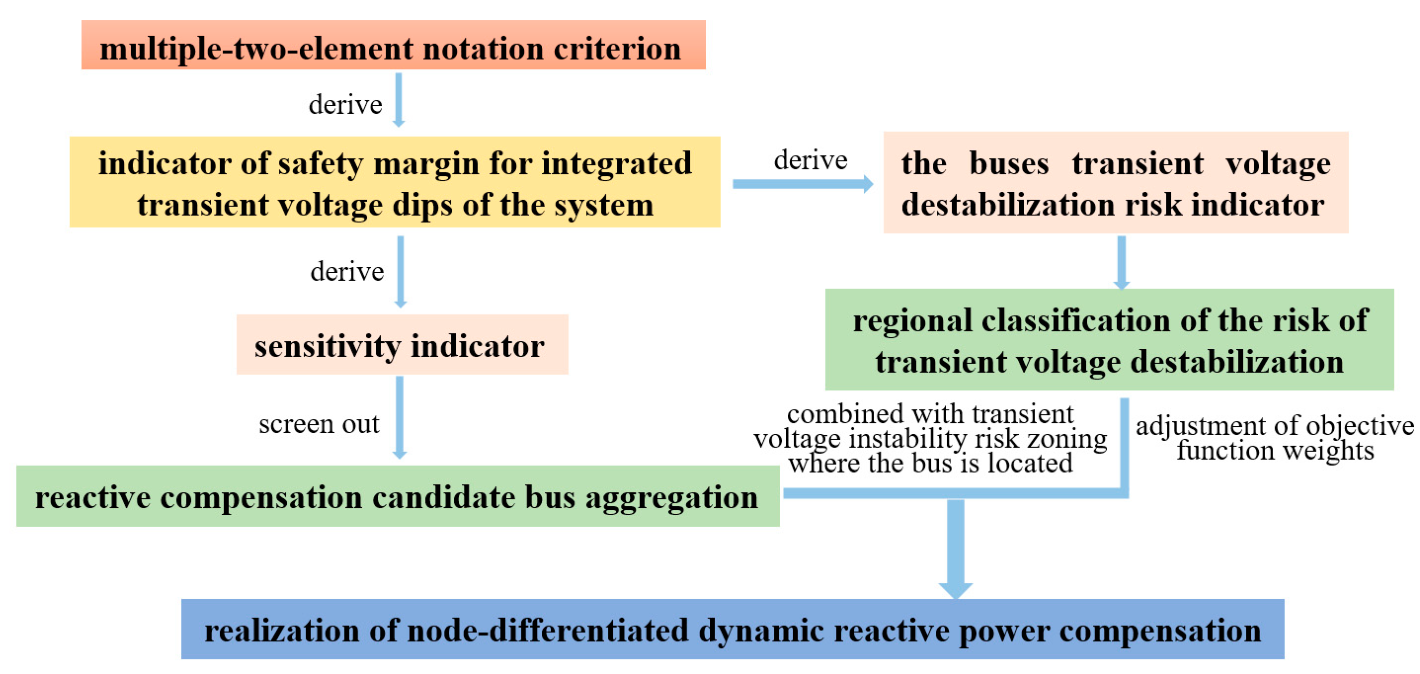
2.6. Relationship and Use of Indicators

In this chapter, we establish a system of indicators for optimizing the configuration of dynamic reactive power compensation devices based on the voltage multi-binary table criterion. The roles and applications of these indicators are as follows:

Firstly, we derive the safety margin Γ from the enhanced voltage multi-binary table criterion. This safety margin quantifies the transient voltage stability of the system and serves as the objective function for the optimal configuration of reactive power compensation devices.

Next, building upon the safety margin Γ, we calculate the sensitivity index and the bus transient voltage instability risk index. These metrics help us identify potential candidate buses for reactive power compensation and categorize regions based on the risk of transient voltage instability.

Finally, we introduce flexibility into the adjustment of the weights assigned to the two sub-objectives: economic efficiency and the effectiveness of reactive power compensation. These adjustments are made in tandem with the level of transient voltage instability risk in the region containing the candidate compensation buses. This approach enables node-specific dynamic reactive power compensation. You can see the relationship between these indicators illustrated in Figure 2.

3. Node-Differentiated Dynamic Reactive Power Compensation Models

3.1. Device Selection

At present, the main application types of dynamic reactive power compensation devices in engineering include synchronous compensator, SVC (Static Var Compensator) and STATCOM (Static Synchronous Compensator), and their performance comparison is shown in

Table 1. Dynamic reactive power compensation device performance comparison.

Term	Synchronous Compensator	SVC	STATCOM
Response time	20 ms	20–60 ms	<10 ms
Active Loss	1.5–5%	0.8%	1%
Overload capacity	strong	weak	weak
Reactive power characteristics	low influence by voltage	proportional to voltage squared	proportional to voltage
Footprint	about 1/3 of SVC	large	about 1/3 of SVC
Investment cost	high	low	low
O and M costs	high	low	low

.

Synchronous compensators are a kind of synchronous rotating equipment to adjust the reactive power output through excitation control, which has the advantages of strong overload capacity, small influence by voltage, and it can provide a rotating moment of inertia, etc. However, the problems in the aspects of high investment and operation and maintenance cost, large active loss, and slow regulation speed before reaching the full-load state are still prominent [14].

SVC and STATCOM are two common types of dynamic reactive power compensation devices widely employed in contemporary power systems. SVC offers several advantages, including the ability to continuously adjust reactive power and a rapid response time. However, it is susceptible to variations in bus voltage. In the event of a severe fault, the output reactive current of SVC can decrease in proportion to the system bus voltage, as described in reference [15]. STATCOM is a new generation of reactive power compensation equipment after SVC, and its output reactive current is not affected by AC bus voltage, but the project cost is higher, and the overall economy is not as good as that of SVC [16]. From the consideration of cost and practical application, SVC and STATCOM are selected for simulation experiments in this paper.

In order to visualize the performance difference between SVC and STATCOM in suppressing the effect of transient voltage dips, a three-phase non-metallic short-circuit fault is set up in a power grid at 0.1 s, and the fault lasts for 0.3 s before it is removed. In the fault bus near the node were configured 300 Mvar SVC and STATCOM. The observation of its reactive power response characteristics and fault bus voltage are shown in Figure 3.

Bo th SVC and STATCOM exhibit the ability to rapidly inject a substantial amount of reactive power during faults, effectively bolstering the transient voltage at the bus. This swift response aids in the speedy restoration of voltage to its normal operating levels and effectively mitigates transient voltage dips. Furthermore, the figure highlights that in the short term, STATCOM outperforms SVC by responding with a greater amount of reactive power at a faster pace. This superior responsiveness results in more pronounced and rapid improvements in reactive power compensation, leading to a more stable and consistent output. In essence, STATCOM’s performance surpasses that of SVC significantly in terms of reactive power compensation effectiveness.

3.2. Configuration Model

The configuration challenge for dynamic reactive power compensation devices fundamentally constitutes a multi-objective optimization problem. Within this optimization problem, cost and reactive power compensation effectiveness serve as the two sub-objective functions. Node-specific compensation is primarily achieved through the flexible adjustment of the optimization weights assigned to these two sub-objectives based on the transient voltage instability risk characteristics of the compensation node. This approach aims to achieve customized compensation while avoiding excessive cost expenditure.

Given that STATCOM offers superior response speed, enhanced reactive power compensation capabilities, and more stable output compared with SVC, it proves highly effective in enhancing the compensation process during pre-transient phases. Nodes exhibiting a high risk of transient voltage instability should prioritize reactive power compensation effectiveness. Therefore, the configuration of STATCOM should be favored to enhance the overall transient voltage dip safety margin of the system and improve its transient stability.

On the other hand, SVC boasts significant economic advantages, allowing for maximum cost savings. Given the substantial installation and operational costs associated with dynamic reactive power devices, nodes with a lower risk of transient voltage instability should place a greater emphasis on economic considerations. In such cases, configuring SVC is preferred, aiming to maximize the economic benefits of the compensation scheme while still meeting the system’s reactive power requirements.

(1)

Objective function

$$f_1={\displaystyle \sum _{i=1}^m(C_{ins-x}+C_{per-x}{Q}_{i-x})}$$

(11)

$$f_2=-\Gamma$$

(12)

$$minF=\{w_1{f}_1,w_2{f}_2\}$$

(13)

f₁ and f₂ are the two sub-objective functions of the multi-objective optimization function F. f₁ is the cost objective function, f₂ is the reactive power compensation effect objective function, and smaller values of f₂ indicate a better reactive power compensation effect; w₁ and w₂ are the optimization weights of the sub-objective functions f₁ and f₂, respectively; and x is the control variable, including the type and the capacity. The coding is shown in Figure 4, where different weights are taken to optimize the n candidate compensation nodes at different risks of transient voltage instability, and the first n bits are used to store the dynamic reactive power compensation device-type judgment variables (0 means no dynamic reactive power compensation device is installed, 1 means that SVC is installed, 2 means that STATCOM is installed), and the last n bits are used to store the configured capacity; the number of dynamic reactive power compensation devices installed is m, C_ins-x is the installation cost, C_per-x is the reactive power compensation unit price, and Q_i-x is the reactive power compensation capacity.

To implement the principle of differentiation, we can assign varying weights to different risk regions. For the high-risk region, we can emphasize the weight of reactive power compensation, resulting in a weight ratio of w₁:w₂ = 1:2, which translates to w₁ = 0.33 and w₂ = 0.67. In the medium-risk region, an equal weight distribution is suitable, yielding w₁:w₂ = 1:1, i.e., w₁ = 0.5 and w₂ = 0.5. In contrast, the low-risk region should prioritize the weight of cost, leading to a weight ratio of w₁:w₂ = 2:1, with w₁ = 0.67 and w₂ = 0.33.

Subsequently, when addressing the differentiated capacity model, we can apply distinct optimization weights to the control variable x, corresponding to different nodes at varying levels of transient voltage instability risk. This approach aligns with the concept of differentiated compensation.

(2)

Constraints

Power balance constraints:

$$\{\begin{array}{l}{U}_i{\displaystyle \sum _{j=1}^{n_b}{U}_j}\left(G_{ij}\cos {\delta }_{ij}+B_{ij}\sin {\delta }_{ij}\right)=P_{Gi}-P_{Li}\hfill \\ U_i{\displaystyle \sum _{j=1}^{n_b}{U}_j}\left(G_{ij}\sin {\delta }_{ij}-B_{ij}\cos {\delta }_{ij}\right)=Q_{Gi}-Q_{Li}\hfill \end{array}$$

(14)

P_Gi, Q_Gi, P_Li and Q_Li are the active and reactive power input and output at the nodes, respectively; U_i is the voltage at the nodes; G_ij is the conductance between branches i-j, B_ij is the conductance between branches i and j, and δ_ij denotes the difference in phase angle between branches i and j; n_b is the total number of nodes; and the reactive and active power inflow and outflow at the nodes in the system should be balanced at all times.

Generator output, nodal voltage, and reactive power capacity constraints:

$$\{\begin{array}{l}{P}_{Gi}^{\min }\le P_{Gi}\le P_{Gi}^{\max }, i=1,2,\cdots ,N\hfill \\ Q_{Gi}^{\min }\le Q_{Gi}\le Q_{Gi}^{\max }, i=1,2,\cdots ,N\hfill \\ U_i^{\min }\le U_i\le U_i^{\max }, i=1,2,\cdots ,N\hfill \\ Q_i^{\min }\le Q_i\le Q_i^{\max }, i=1,2,\cdots ,n\hfill \end{array}$$

(15)

$P_{Gi}^{\max }$, $P_{Gi}^{\min }$ and $Q_{Gi}^{\max }$, $Q_{Gi}^{\min }$ denote the upper and lower limits of the node input active and reactive power, respectively; $U_i^{\max }$, $U_i^{\min }$ and $Q_i^{\max }$, $Q_i^{\min }$ are the upper and lower limits of the voltage and reactive power compensation capacity, respectively.

The above equation constrains the limits of generator active reactive power output, reactive power compensation output, and nodal voltage in each node to prevent the occurrence of relevant power and voltage overruns, respectively.

4. Solving Algorithm and Process

4.1. ETLBO Optimization Algorithm

The TLBO (Teaching–Learning-Based Optimization) algorithm is a novel intelligent algorithm that mimics the dynamics of a classroom teaching environment. It offers advantages such as simplicity due to its minimal parameter requirements, ease of implementation, and rapid convergence. However, it also exhibits certain drawbacks, including a tendency to become trapped in local optima and a significant reduction in convergence speed as the number of dimensions increases [17].

To address these limitations, the enhanced ETLBO (Elitist Teaching–Learning-Based Optimization) algorithm incorporates elite strategies into the core TLBO framework. This modification accelerates algorithm convergence and significantly reduces the risk of falling into local optima. Importantly, this improved algorithm closely follows the main processes of the TLBO algorithm and proves to be particularly well-suited for optimizing the allocation of dynamic reactive power compensation [18]. The primary processes are as follows:

• Initialization

First set the number of iterations, the number of students in the class, and the number of subjects to randomly initialize the class students to generate a class population as follows:

$$\left[\begin{array}{cc}{X}_1& f\left(X_1\right)\\ X_2& f\left(X_2\right)\\ ⋮& ⋮\\ X_N& f\left(X_N\right)\end{array}\right]=\left[\begin{array}{ccccc}{x}_{11}& x_{12}& \cdots & x_{1d}& f\left(X_1\right)\\ x_{21}& x_{22}& \cdots & x_{2d}& f\left(X_2\right)\\ \cdots & \cdots & \cdots & \cdots & \cdots \\ x_{N1}& x_{N2}& \cdots & x_{Nd}& f\left(X_N\right)\end{array}\right]$$

(16)

f(X_i) is the value of the objective function for individual X_i; N is the population size, i.e., the number of individuals in the class. X_i denotes the ith individual, X_i = (x_i1, x_i2, …, x_id,), where d is the dimension of each individual student.

b.

“Teaching” process

In the “teaching” process, the “difference” between the teacher and the learner is calculated to promote the learner to approach the teacher to improve the learner’s knowledge, as shown in Equation (17):

$$X_i^{\prime }=X_i+D=X_i+r(X_{teacher}-T_F{X}_{Mean})$$

(17)

X_i′ is the new trainee generated by trainee X_i after the “teaching” process; X_teacher is the teacher, X_Mean is the average value of the trainees in the class, and r is a random number with a value ranging from 0 to 1. T_F stands for Teaching Factor, whose value is taken as one or two. After the “teaching” process, the “grades” of the old and new learners are compared and the one with better grades is retained.

c.

“Self-learning” process

This process ensures population diversity through mutual learning between individual participants in the form of communication, group discussion, etc., with the formula:

$$X_i^{\prime }=\{\begin{array}{ll}{X}_i+r(X_i-X_i)\hfill & f(X_i)<f(X_i)\hfill \\ X_i-r(X_i-X_j)\hfill & f(X_i)>f(X_j)\hfill \end{array}$$

(18)

X_i′ is the new learner generated by learner X_i after the “self-study” process; X_j is a randomly selected other learner; and r is a random number with a value ranging from 0 to 1. Similarly, after the “self-study” process, the better of the old and new trainees are retained.

In this paper, the ETLBO algorithm is used to calculate the type and capacity of dynamic reactive power compensation devices and is solved to derive the set of schemes for dynamic reactive power compensation device configuration.

4.2. TOPSIS Evaluation Method

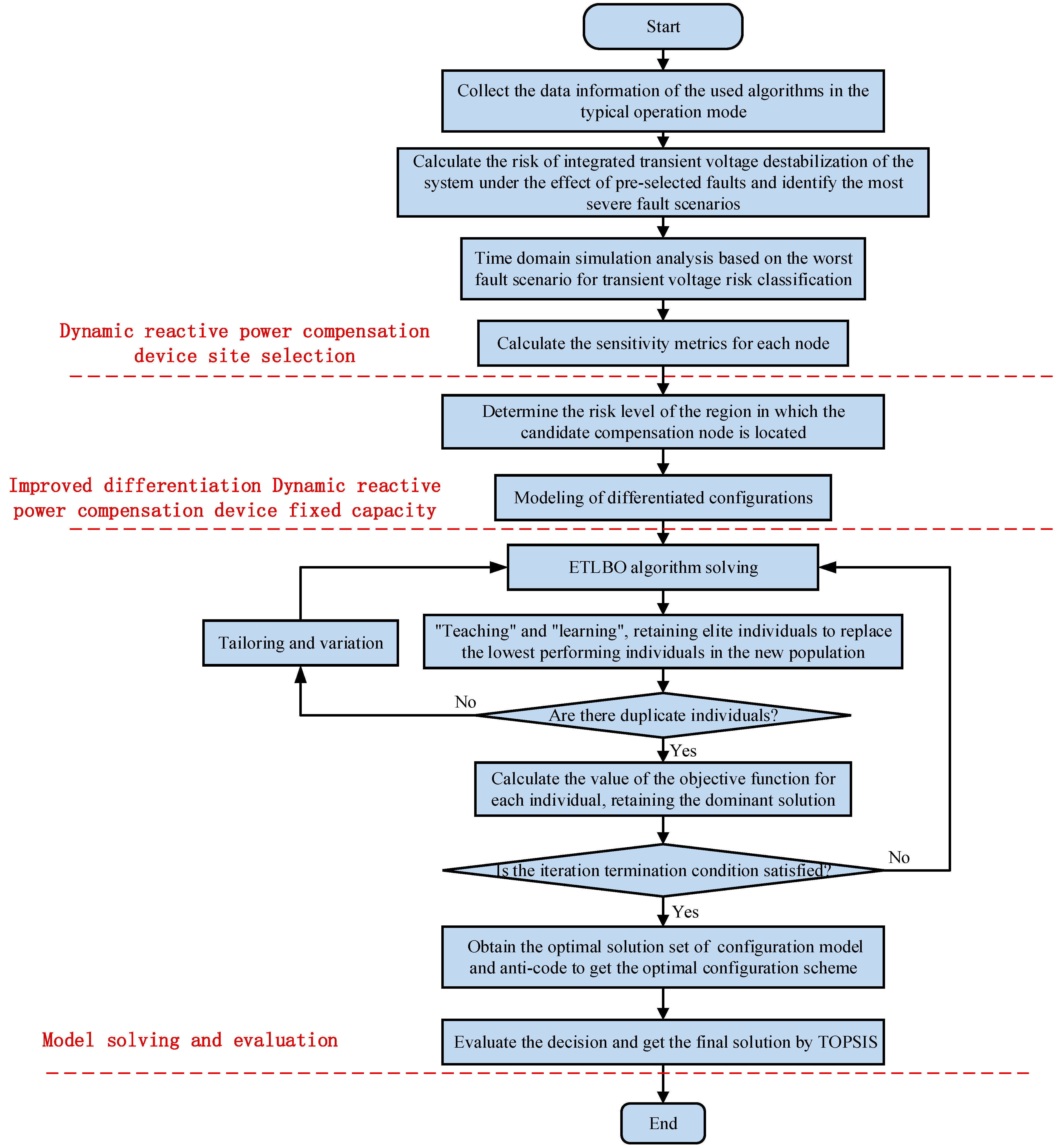
The ETLBO algorithm yields an optimal solution for the objective function, resulting in a set of non-inferior solution sets positioned along the Pareto front. To choose the optimal configuration scheme from these solutions, it is necessary to assess and rank the optimization results. The TOPSIS (Technique for Order Preference by Similarity to Ideal Solution) method, also referred to as the ideal solution approximation method, is a multi-attribute decision-making technique based on evaluating the relative merits and demerits of existing objects in proximity to an idealized target [19]. The calculation proceeds as follows:

Let there be m evaluation objectives D_i = {D₁, D₂,···, D_m} in the multi-objective optimization problem, and each evaluation objective contains n evaluation indexes x_j = {x₁, x₂,···, x_n}; then, we can establish the feature matrix of the evaluation objectives D, in which D_i(x_j) = x_ij. The elements in the feature matrix are uniformly normalized as shown in Equation (19).

$$r_{ij}=\frac{x_{ij}}{\sqrt{{\displaystyle \sum _{i=1}^m{x}_{ij}^2}}}$$

(19)

Establish the normalization matrix v_ij as shown in Equation (20), where w_j is the weight of the jth indicator in the normalization matrix v_ij.

$$v_{ij}= w_j{r}_{ij}, i=1,2,\cdots ,m,j=1,2,\cdots ,n$$

(20)

Ideal solution A and negative ideal solution A can be represented by the normalized matrix v_ij with weights; J₁ and J₂ are the highest value and the lowest value of weights on the ith evaluation objective, respectively.

$$\begin{array}{l}{A}^{+}=\{v_1^{+},v_2^{+},\cdots ,v_m^{+}\},v_j^{+}=\{\underset{i}{\max }{v}_{ij},j\in J_1;\underset{i}{\min }{v}_{ij},j\in J_2\}\\ A^{-}=\{v_1^{-},v_2^{-},\cdots ,v_m^{-}\}, v_j^{-}=\{\underset{i}{\min }{v}_{ij},j\in J_1;\underset{i}{\max }{v}_{ij},j\in J_2\}\end{array}$$

(21)

The smaller the distance between the solution to be evaluated and the ideal solution, i.e., the larger the distance between the solution and the negative ideal solution, the more optimal the solution is. Calculate the distance between each program to be evaluated and the positive and negative ideal solutions and solve for the closeness P_i; the program with the largest closeness value is the optimal program sought.

$$\{\begin{array}{c}{P}_{\mathrm{i}}=\frac{S_i^{-}}{S_i^{+}+S_i^{-}}\hfill \\ S_i{}^{+}=\sqrt{{\displaystyle \sum _{j=1}^n{(v_j^{+}-v_{ij})}^2}}\hfill \\ S_i{}^{-}=\sqrt{{\displaystyle \sum _{j=1}^n{(v_j^{-}-v_{ij})}^2}}\hfill \end{array}$$

(22)

In the configuration schemes proposed in this paper, there are two evaluation objectives: the effectiveness of reactive power compensation Γ and investment cost. When assessing the reactive power compensation effectiveness Γ, the ideal solution represents the maximum value of Γ among all alternatives, while the negative ideal solution is the minimum value. Conversely, for the cost evaluation objective, the ideal solution signifies the minimum cost among all alternatives, while the negative ideal solution is the maximum cost. The process involves calculating the distances between each alternative and the positive and negative ideal solutions, determining their closeness, and ultimately identifying the solution with the highest closeness value as the sought-after optimal solution.

4.3. Solution Steps

The configuration process for dynamic reactive power compensation devices involves the following steps:

(1)

Trend Calculation and Weight Coefficients: Initiate the algorithm by conducting trend calculations through PSD-BPA. Collect system trend information and calculate the weight coefficients for each bus.

(2)

N-1 Fault Scanning: Conduct N-1 fault scanning across the system. Calculate the integrated transient voltage instability risk D_Γ,l for the system under the influence of pre-selected faults. Rank these risks to determine the benchmark scenario for reactive power planning, focusing on the most severe faults.

(3)

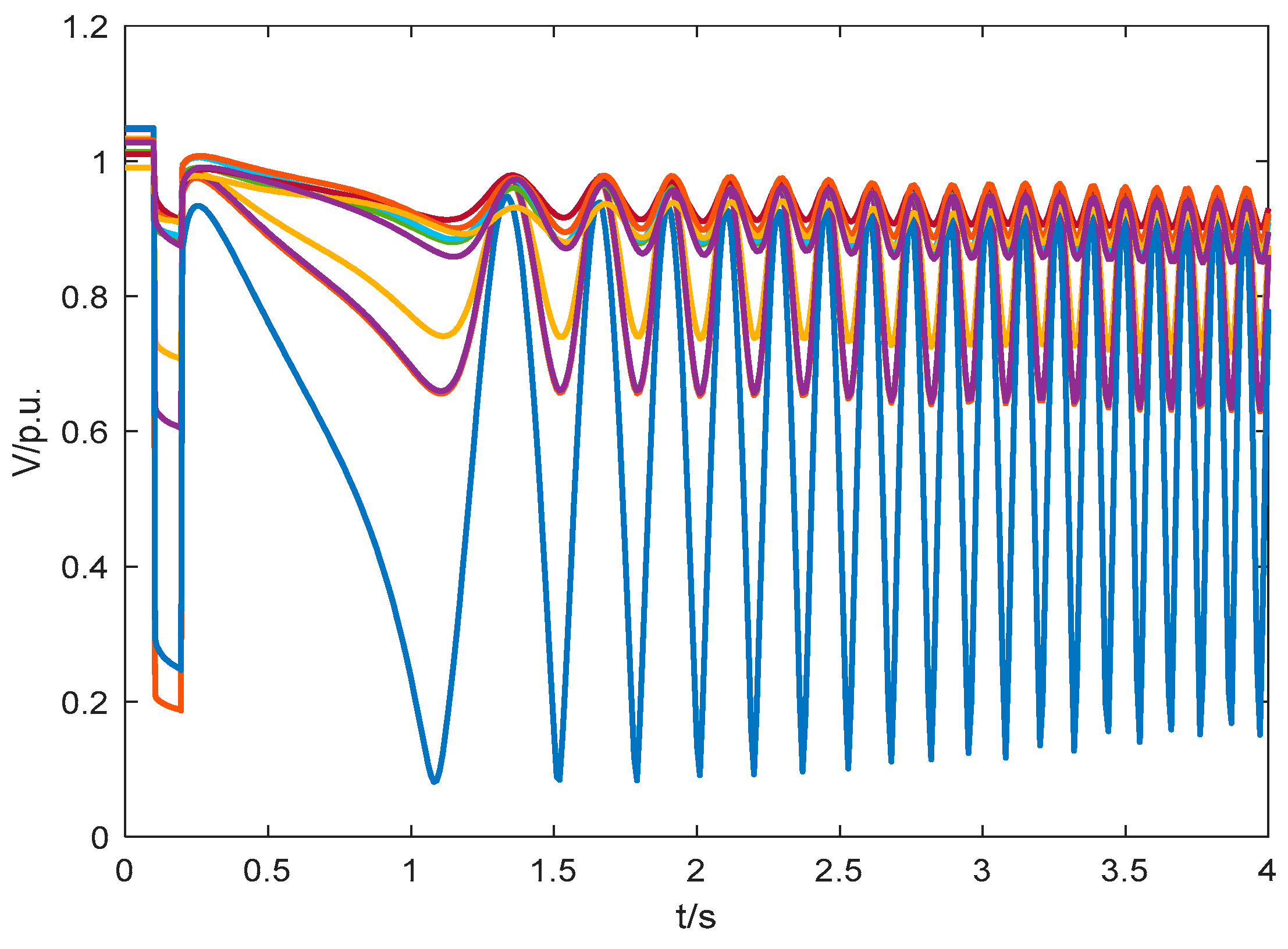
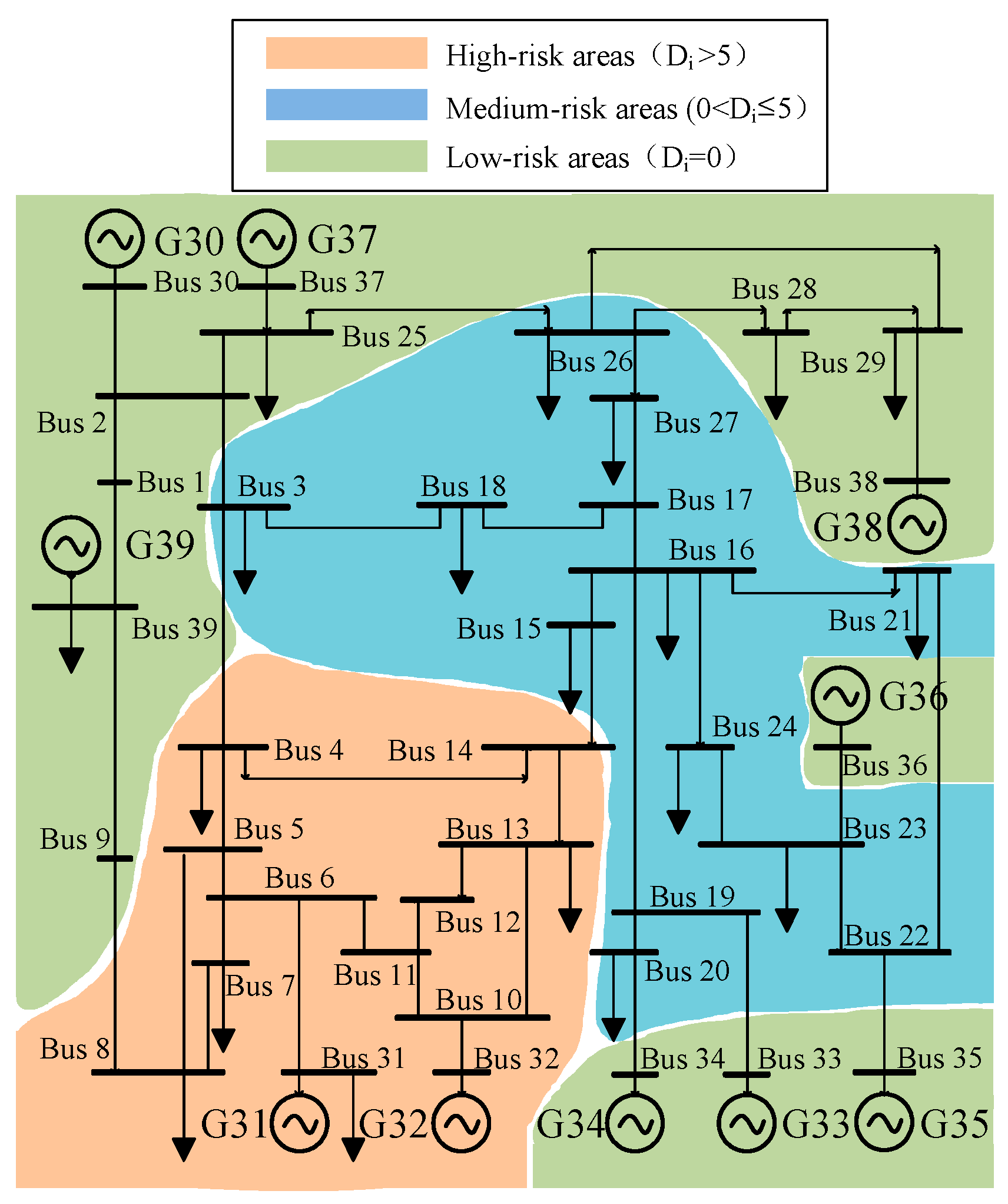
Transient Voltage Instability Analysis: Perform time domain simulation analysis based on the benchmark scenario for the most severe fault. Calculate the transient voltage instability risk index D_i for each node and categorize them into regions with varying levels of risk: high-, medium-, and low risk of transient voltage instability.

(4)

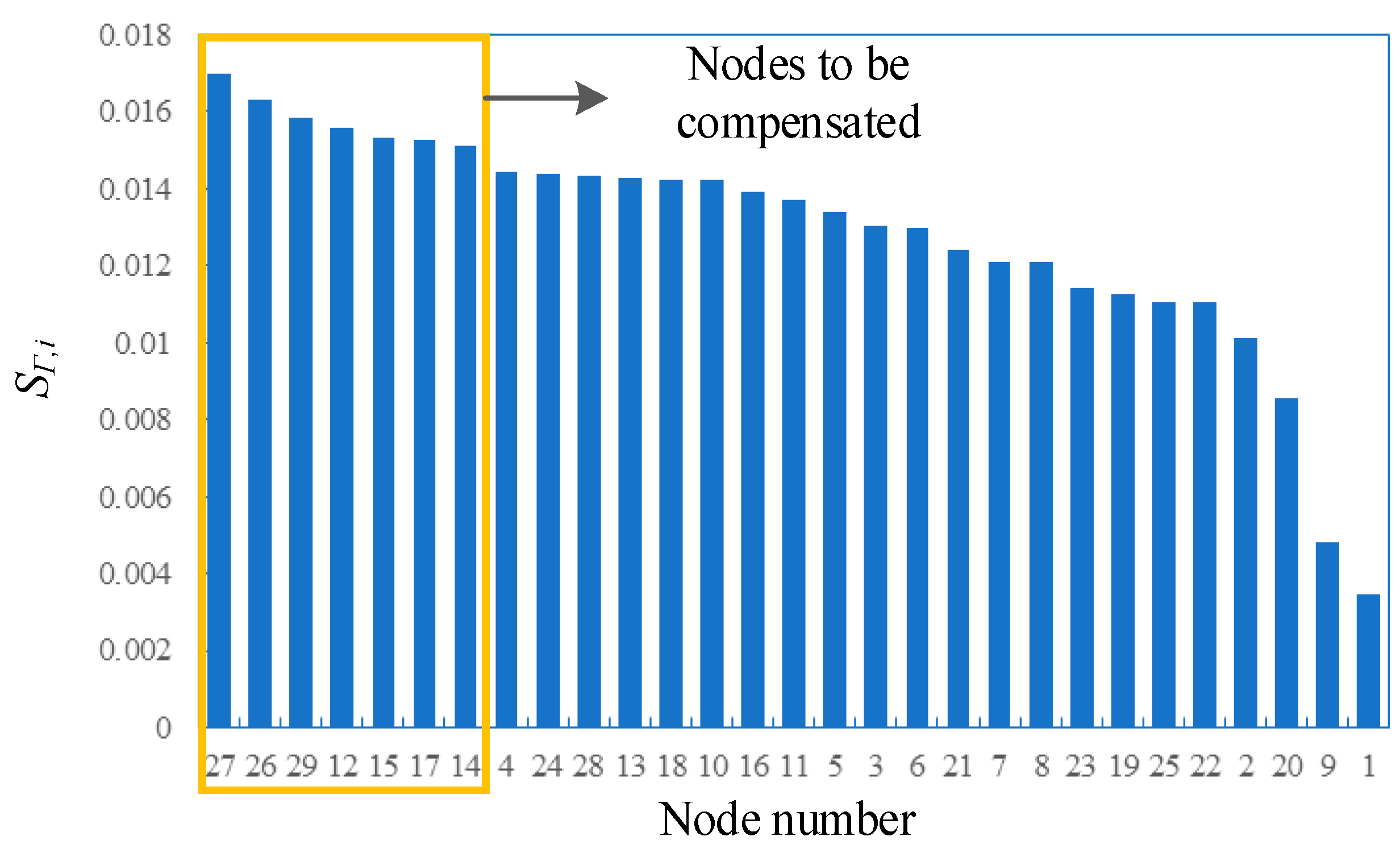
Sensitivity Analysis: Continue with the most severe fault scenario and sequentially connect dynamic reactive power compensation devices of the same type and capacity to each node in the system. Conduct time domain simulation analysis and calculate the sensitivity index S_Γ,i for each node. Construct a set of candidate nodes based on S_Γ,i.

(5)

Candidate Node Determination: Based on the locations of the identified candidate nodes for reactive power compensation, determine the transient voltage instability risk regions they belong to. Combine the optimization weights for each selected reactive power compensation node. Encode the type and capacity of the dynamic reactive power compensation devices. Utilize optimization algorithms to differentially solve the problem and obtain a set of candidate solutions.

(6)

Evaluation and Selection: Utilize the TOPSIS evaluation decision method to assess the potential scenarios for configuring dynamic reactive power compensation devices under the established baseline scenario. Select the final scenario based on the evaluation results.

The corresponding general flow of dynamic reactive power device configuration is shown in Figure 5

5. Example Analysis

In this section, the IEEE39 node system is used as an example for simulation and analysis, and the system wiring diagram is shown in Figure 6. The branch, node, transformer, and generator parameters of the system are shown in the literature [20] and are simulated by applying Matlab and PSD-BPA software. All the loads are configured in a ratio of 50% constant impedance and 50% induction motor, and the load model parameters are referred to in the literature [21]. Considering the typicality of the algorithm and the computational volume, this paper considers the installation of dynamic reactive power compensation devices at six nodes, i.e., the dimension of the type variable n = 6 and the total dimension of the decision variable 2n = 12.

5.1. Candidate Compensation Nodes

(1)

Filtering the set of worst failures

The problem of dynamic reactive power compensation device placement and capacity setting is an integer nonlinear programming problem, and in order to reduce the amount of computation, it is necessary to determine in advance the severe faults that may occur in the system. In order to simplify the processing, this algorithm examines the three-phase short-circuit fault situation, and sets the probability of faults occurring in each line to be equal. There are 46 lines in the IEEE39 system, so there are a total of 46 fault scenarios. A three-phase short-circuit is set to occur on the line at the moment of t = 0.1 s, and the duration of the fault is set to be 0.1 s. The fault is set to be a three-phase short-circuit grounding of all transmission lines within the sub-district at the 50% position of the line in sequence, and the fault disappears after 0.1 s. The time interval included in the index calculation is 0.1~2.0 s, i.e., within 1.9 s after the fault appears; the sampling interval of voltage magnitude is 0.02 s; and the weights of each moment are all 1. According to the simulation results, the system voltage instability risk index D_Γ,l is calculated using Equation (4) for each fault, and it can be seen from the analysis in Section 2.3 that the bigger D_Γ,l is, the more likely that the system will have voltage instability, and the results are as follows in

Table 2. D_Γ,l under the set of failures.

Failure Number	DΓ,l	Failure Number	DΓ,l	Failure Number	DΓ,l
1	0.0909	17	0.9490	33	0.2714
2	0.0796	18	0.9148	34	1.7133
3	0.4212	19	0.7055	35	0.8796
4	0.4380	20	0.8705	36	0.3278
5	0.6902	21	0.9528	37	0.5423
6	0.4949	22	0.6184	38	0.6378
7	0.8572	23	0.6772	39	0.3311
8	0.8787	24	0.8356	40	0.2553
9	0.9739	25	0.6696	41	0.3781
10	0.8299	26	0.4717	42	0.2440
11	0.8614	27	0.5254	43	0.1699
12	0.9562	28	0.5051	44	0.2006
13	0.7955	29	0.3624	45	0.2976
14	0.3163	30	0.3121	46	0.3557
15	0.0928	31	0.3784
16	0.9501	32	0.2797

:

As can be seen from Table 2, the risk of system transient voltage destabilization is different for faults occurring in different lines, and the impact of three-phase short-circuit faults occurring in some lines on the system transient voltage is small, such as fault 2 and so on. In this paper, the eight most serious faults are selected as the most serious fault set, i.e., faults numbered 34, 9, 12, 21, 16, 17, 18, and 35, which correspond to the actual faults of bus-28 and bus-29 lines, bus-05 and bus-06 lines, bus-06 and bus-11 lines, bus-10 and bus-11 lines, bus-16 and bus-17 lines, bus-10 and bus-13 lines, bus-13 and bus-14 lines, and bus-11 and bus-12 lines at the midpoint of the three-phase ground short circuit. Taking the three-phase short circuit of bus-28 and bus-29 lines as an example, different buses are marked with different colors and some of the bus voltages of the system are shown in Figure 7:

(2)

Candidate nodes

Similarly, preselecting candidate installation nodes for reactive power compensation devices significantly reduces the computational workload of the example and enhances the project’s practicality. Typically, dynamic reactive power compensation devices are not installed at busbars where synchronous generators are located. Hence, this paper exclusively considers the installation of reactive power devices at nodes without generators.

To assess the impact of installing reactive power devices with the same capacity at different nodes in mitigating transient voltage instability, we take an example where a 50 MVar STATCOM device is configured at each node within the system. The integrated transient voltage dip safety margin index Γ for the system after compensation at each node is computed under the scenario of the most severe fault set. Subsequently, the corresponding sensitivity index is derived, as outlined in

Table 3. Comparison of metrics for candidate compensation nodes.

Nodal	Γ	SΓ,i	Nodal	Γ	SΓ,i
1	−5.48855	0.003469	16	−4.96675	0.013905
2	−5.15575	0.010125	17	−4.8989	0.015262
3	−5.0114	0.013012	18	−4.9498	0.014244
4	−4.9407	0.014426	19	−5.09815	0.011277
5	−4.99185	0.013403	20	−5.23305	0.008579
6	−5.0139	0.012962	21	−5.04085	0.012423
7	−5.05725	0.012095	22	−5.10995	0.011041
8	−5.05815	0.012077	23	−5.0916	0.011408
9	−5.4201	0.004838	24	−4.94405	0.014359
10	−4.9501	0.014238	25	−5.1098	0.011044
11	−4.97635	0.013713	26	−4.84815	0.016277
12	−4.8839	0.015562	27	−4.8134	0.016972
13	−4.947	0.0143	28	−4.9461	0.014318
14	−4.9066	0.015108	29	−4.8698	0.015844
15	−4.89625	0.015315

:

The corresponding sensitivity index S_Γ,i for each node is shown in Figure 8:

From Figure 8, it can be seen that the effects of installing reactive power compensation devices with the same capacity at different nodes on reducing the risk of transient voltage instability are different, and the installation of reactive power compensation devices at some nodes can more significantly inhibit the occurrence of transient voltage instability. In this paper, six nodes with the largest sensitivity indexes are selected as the candidate nodes for dynamic reactive power compensation device installation, which are nodes 27, 26, 29, 12, 15, and 17.

5.2. System Transient Voltage Instability Risk Partitioning

Once the candidate compensation nodes of the system are known, the instability risk of the selected reactive power compensation nodes can be determined for the region in which they are located in the system, and their optimization weights can be determined to achieve differentiated dynamic reactive power compensation. Also based on the worst fault set scenario, the transient voltage instability risk indicator D_i is calculated for each node of the system and the number of instabilities of the node is counted, as shown in

Table 4. Indicators of risk of node destabilization.

Nodal	Di	Number of Instabilities	Nodal	Di	Number of Instabilities	Nodal	Di	Number of Instabilities
1	0.0000	0	14	16.7118	6	27	1.7394	1
2	0.0000	0	15	4.2450	3	28	0.0000	1
3	0.5803	1	16	2.5523	1	29	0.0000	1
4	11.7646	6	17	2.3568	1	30	0.0000	0
5	10.3804	6	18	2.0995	1	31	7.3380	5
6	10.6489	6	19	1.5516	1	32	7.4773	5
7	9.9658	5	20	1.4768	1	33	0.0000	0
8	9.5830	5	21	2.1258	1	34	0.0000	0
9	0.0000	0	22	1.6480	1	35	0.0000	0
10	11.2007	6	23	1.7070	1	36	0.0000	0
11	11.5400	6	24	2.6959	1	37	0.0000	0
12	11.2962	6	25	0.0000	0	38	0.0000	0
13	10.8595	6	26	0.3354	2	39	0.0000	0

.

In all the worst fault set scenarios, nodes with D_i ≥ 5 have at least five transient voltage destabilizations; nodes with 0 < D_i ≤ 5 have at most three voltage destabilizations, and most of them have only one destabilization; and nodes with D_i ≥ 5 have transient voltages that remain stable. Based on this, the nodes with D_i = 0 are located in low-risk areas; nodes with 0 < D_i ≤ 5 are located in medium-risk areas; and nodes with D_i ≥ 5 are located in high-risk areas. The risk zoning of transient voltage instability in the IEEE39 system is shown in Figure 9 below:

From the figure, it can be seen that most of the nodes containing generators are located in low-risk areas, and the risk of instability of nodes that are electrically distant from generators is generally relatively high, which is closely related to the ability of generators to quickly provide voltage support and maintain system stability.

5.3. Configuration Results

As can be seen from Figure 8, the proposed compensation nodes for the six selected dynamic reactive power compensation devices are nodes 27, 26, 29, 12, 15, and 17. Combined with Figure 9, the six compensation nodes are classified into risk areas: nodes 12 and 15 are in the high-risk area, and nodes 27, 26, and 17 are in the medium-risk area. Node 29 is in the low-risk region.

The candidate dynamic reactive power compensation devices include SVC and STATCOM, with their parameters set to match the equipment used in the actual project. The fixed installation costs and compensation unit prices for SVC and STATCOM devices are detailed in

Table 5. Economic parameters and investment costs of dynamic reactive power compensation devices.

Device Type	Operational Life/a	Installation Costs/USD	Reimbursement Unit Price/[USD∙Mvar−1]
SVC	10	1.3 × 107	3 × 104
STATCOM	10	2.6 × 107	9 × 104

. In comparing the traditional dynamic reactive power compensation method with the improved differentiated method, the former lacks an analysis of transient voltage instability risk at the compensation node and lacks the link to adjust optimization weights for cost and suppression effect. The remainder of the process aligns with the differentiated compensation approach. The selection of dynamic reactive power compensation devices and the determination of their capacities are executed at the selected compensation nodes according to both the traditional and improved differentiated methods presented in this paper. The results obtained through the multi-objective optimization algorithm solution are displayed in

Table 6. Results of the two compensation methods.

Method	Scheme	Cost/USD	Γ
Differential compensation	1	2.3769 × 108	3.9567
	2	1.6360 × 108	3.5939
	3	1.4310 × 108	2.7685
	4	1.5268 × 108	3.1681
	5	2.5398 × 108	3.9922
Traditional compensation	1	2.3295 × 108	3.8017
	2	2.2608 × 108	3.6932
	3	1.7659 × 108	2.9846
	4	1.6186 × 108	2.8461
	5	1.4974 × 108	2.7926

and Figure 10.

Firstly, when examining the figure as a whole, it is evident that the configuration cost of the dynamic reactive power compensation device is positively correlated with its reactive power compensation effectiveness. Increasing the configured capacity can effectively enhance the compensation effect of the dynamic reactive power compensation device, albeit at a higher cost.

Secondly, focusing on the specific curve, the results obtained through the differentiated dynamic reactive power compensation method proposed in this paper notably outperform the traditional compensation method in terms of overall economy. This improvement is attributed to the optimization weight differentiation at nodes. For nodes within the medium- and low-risk regions, the optimization weight for the reactive power compensation effectiveness index is appropriately reduced, while cost considerations are balanced. This approach ensures that the configuration of the dynamic reactive power compensation device not only meets the system’s reactive power compensation requirements, but also achieves greater cost efficiency.

Lastly, observing the curve’s trend reveals a certain saturation point between reactive power compensation effectiveness and cost. Beyond a certain capacity threshold for the dynamic reactive power compensation device, the enhancement in compensation effectiveness becomes less pronounced, leading to increased cost burdens. Hence, it is essential to conduct a comprehensive assessment of the configuration results obtained through multi-objective optimization to select the most rational configuration scheme, achieving a balanced optimization of economy and reactive power compensation effectiveness.

The inverse coding of the optimization solution set using the differentiated dynamic reactive power compensation method yields the capacity configuration scheme and evaluation of the dynamic reactive power compensation device, as displayed in

Table 7. Configuration schemes.

Compensation Node	Scheme 1		Scheme 2		Scheme 3		Scheme 4		Scheme 5
	Capacity /Mvar	Type	Capacity /Mvar	Type	Capacity /Mvar	Type	Capacity /Mvar	Type	Capacity /Mvar	Type
Bus-12	463	SVC	372	STATCOM	438	SVC	306	STATCOM	433	SVC
Bus-15	453	STATCOM	255	SVC	225	SVC	206	SVC	460	STATCOM
Bus-17	478	SVC	456	SVC	114	SVC	300	SVC	418	STATCOM
Bus-26	238	STATCOM	310	SVC	363	SVC	240	SVC	91	SVC
Bus-27	406	SVC	402	SVC	395	SVC	397	SVC	454	SVC
Bus-29	201	STATCOM	115	SVC	85	SVC	195	SVC	318	STATCOM

and

Table 8. Evaluation of the configuration schemes.

Scheme	Cost/USD	Γ	Closeness Value
1	2.3769 × 108	3.9567	0.4179
2	1.6360 × 108	3.5939	0.7707
3	1.4310 × 108	2.7685	0.6202
4	1.5268 × 108	3.1681	0.6894
5	2.5398 × 108	3.9922	0.3798

.

From Table 7, which presents the selection of dynamic reactive power compensation device types and capacity configurations, it is evident that, for economic considerations, there are significantly more compensation nodes selected for SVC installation compared with STATCOM. Additionally, the individual node installation capacity of STATCOM consistently remains lower than that of SVC. This observation suggests that STATCOM can provide a substantial amount of reactive power for compensation with a smaller capacity, showcasing its superior reactive power support capability compared with SVC. Furthermore, all compensation nodes chosen for STATCOM installation are within the high-risk area of transient voltage instability. This underscores that the differentiated compensation method proposed in this paper can fulfill the required reactive power compensation effect based on node risk characteristics while simultaneously enhancing the overall system economy.

The evaluation results for each candidate scheme in Table 7 using the TOPSIS method are summarized in Table 8. Among these schemes, Scheme 5 offers the best reactive power compensation effect, but also incurs the highest cost. In contrast, Scheme 3 achieves optimal economy but falls short in terms of reactive power compensation effectiveness. Therefore, Scheme 2, with the highest closeness index, should be selected as the final configuration scheme.

Based on the optimization results obtained through the traditional dynamic reactive power compensation method and the differentiated method presented in this paper, the corresponding types and capacities of dynamic reactive power compensation devices are installed at the selected compensation nodes under the most severe fault scenarios. The integrated transient voltage dip safety margin indexes of the system before and after dynamic reactive power compensation are calculated (Γ and node instability), and the results are displayed in

Table 9. Comparison of costs and effectiveness of compensation methods.

Method of Compensation	Cost/USD	Γ	Total Number of Instabilities
Uncompensated	0	−5.6620	106
Traditional compensation method	2.1008 × 108	3.6032	78
Differentiated compensation method	1.6360 × 108	3.5939	79

.

As observed in Table 9, under the worst-case fault scenario, the installation of dynamic reactive power compensation devices significantly enhances safety margins and drastically reduces the instances of transient voltage instability in the system when compared with the original example without any reactive power compensation. Both compensation methods reduce the instances from 106 to 78 and 79 times, respectively. Additionally, the safety margin Γ improves from −5.6620 to 3.6032 and 3.5939, respectively. This demonstrates that the dynamic reactive power compensation methods proposed in this paper effectively achieve the goal of suppressing the risk of transient voltage instability in the system.

Comparing the results of the two dynamic reactive power compensation methods, the differentiated dynamic reactive power compensation method based on node characteristics is on par with the traditional method in terms of enhancing system stability and suppressing the risk of transient voltage instability. The safety margin Γ values are similar, with a total number of instabilities of 78 and 79. However, there is a substantial improvement in terms of economy, with costs reduced from 2.1008 × 10⁸ USD to 1.6360 × 10⁸ USD in the traditional method, representing a 22.13% decrease. The differentiated compensation method, based on node risk characteristics, can yield significant cost savings and deliver high economic benefits in practical engineering applications.

6. Conclusions

Based on the voltage multiple-two-element notation criterion, this paper proposes a differentiated dynamic reactive power compensation device configuration scheme to minimize the investment cost of reactive power compensation and improve the risk suppression effect of transient voltage instability. The conclusions are as follows:

(1)

A dynamic reactive device configuration index system based on multiple binary tables is proposed, and the corresponding differentiated dynamic reactive power compensation model is established under this system, which reduces the investment cost of reactive power compensation and increases the economic benefits.

(2)

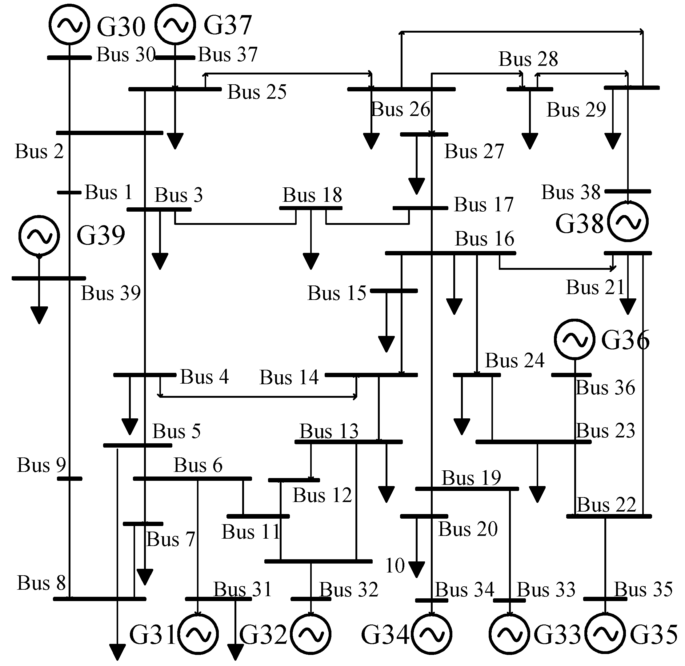
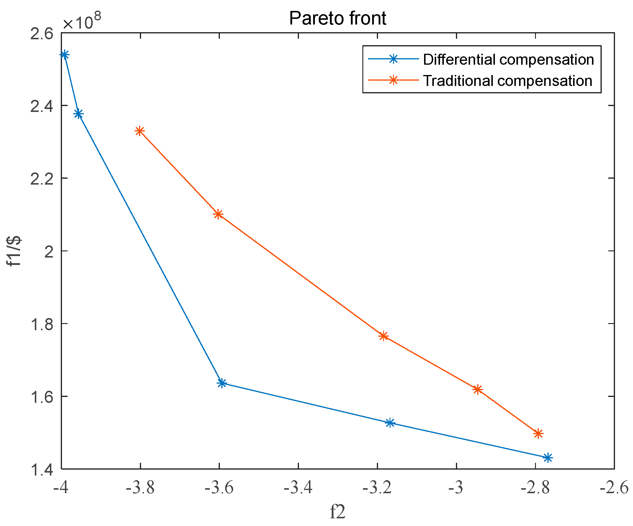
The improved algorithm of ETLBO is used to optimize the model in the IEEE39 system, and the configuration scheme that satisfies the optimization objective is obtained. The TOPSIS evaluation method is used for evaluation and the optimal scheme 2 with the highest score is selected as the final scheme. Compared with the traditional method, the differentiated compensation method compensates similarly and reduces the cost by 22.13%.

References

1. Sami, M.; Gheorghe, S.; Toma, L. Transient stability improvement and voltage regulation in power system hosting Renewables by SVC. In Proceedings of the 2022 International Conference on Electrical, Computer and Energy Technologies (ICECET), Prague, Czech Republic, 20–22 July 2022; pp. 1–7. [Google Scholar]
2. Opana, S.; Charles, J.K.; Nabaala, A. STATCOM Application for Grid Dynamic Voltage Regulation: A Kenyan Case Study. In Proceedings of the 2020 IEEE PES/IAS PowerAfrica, Nairobi, Kenya, 25–28 August 2020; pp. 1–5. [Google Scholar]
3. Zhang, J.; Lin, W.; Zhang, B.; Mei, Y.; Li, J.; Wu, X.; Zhu, L. Research on Dynamic Reactive Power Compensation Configuration of High Proportion New Energy Grid. In Proceedings of the 2020 5th Asia Conference on Power and Electrical Engineering (ACPEE), Chengdu, China, 4–7 June 2020; pp. 2002–2006. [Google Scholar]
4. Zhang, Y.; Zhang, Y.; Jian, W.; Tang, F. Optimal Configuration Method of Dynamic Reactive Power Compensation Device Considering Reducing Commutation Failure Risk of Multi-infeed DC System. In Proceedings of the 2020 IEEE 4th Conference on Energy Internet and Energy System Integration (EI2), Wuhan, China, 30 October–1 November 2020; pp. 3233–3237. [Google Scholar]
5. Cui, J. Research on Transient Voltage Characterization and Control of AC and DC Power Grids. Master’s Thesis, North China Electric Power University, Beijing, China, 2020. [Google Scholar]
6. National Energy Administration. Technical Specification for Power System Safety and Stability Calculation; China Electric Power Press: Beijing, China, 2013; p. 15. [Google Scholar]
7. China Southern Power Grid Co. Guidelines for Calculation and Analysis of Safety and Stability of the Southern Power Grid; China Southern Power Grid Co.: Guangzhou, China, 2009; p. 8. [Google Scholar]
8. Overbye, T.J.; Klump, R.P. Effective Calculation of Power System Low-Voltage Solutions. IEEE Trans. 1996, 11, 75–82. [Google Scholar] [CrossRef]
9. Wildenhues, S.; Rueda, J.L.; Erlich, I. Optimal allocation and sizing of dynamic var sources using heuristic optimization. IEEE Trans. Power Syst. 2015, 30, 2538–2546. [Google Scholar] [CrossRef]
10. Zhou, Q.; Zhang, Y.; He, H. A practical site selection method for dynamic reactive power compensation in multi-infeed DC power grid. Power Syst. Technol. 2014, 38, 1753–1757. [Google Scholar]
11. Xue, A.; Zhou, J.; Liu, R. Research on practical transient voltage stability margin index using multiple binary table criterion. Chin. J. Electr. Eng. 2018, 38, 4117–4125+4317. [Google Scholar]
12. Liu, Z.; Zhang, Q.; Wang, Y. Research on reactive power compensation measures to improve the safety and stability level of 750 kV sending end power grid in Northwest New Ganqing. Chin. J. Electr. Eng. 2015, 35, 1015–1022. [Google Scholar]
13. Xu, Y.; Jiang, W.; Sun, S. Quantitative assessment method of transient voltage in distribution network containing high penetration wind power. China Electr. Power 2022, 55, 152–162. [Google Scholar]
14. Xu, Z.; Chen, Y.; Zhai, B.; Chen, G.; Yang, Q.; Chen, J. A Comparative Study of the Virtual Synchronous Compensator on the Voltage Stability Enhancement. In Proceedings of the International Conference on Renewable Energies and Smart Technologies (REST), Tirana, Albania, 28–29 July 2022; pp. 1–5. [Google Scholar]
15. Eltamaly, A.M.; El-Sayed, A.-H.M.; Mohamed, Y.S.; Elghaffar, A.N.A. A Modified Techniques of Transmission System by Static Var Compensation (SVC) for Voltage Control. In Proceedings of the 2019 8th International Conference on Modeling Simulation and Applied Optimization (ICMSAO), Manama, Bahrain, 15–17 April 2019; pp. 1–5. [Google Scholar]
16. Yarlagadda, V.; Garikapati, A.K.; Gadupudi, L.; Kapoor, R.; Veeresham, K. Comparative Analysis of STATCOM and SVC on Power System Dynamic Response and Stability Margins with time and frequency responses using Modelling. In Proceedings of the 2022 International Conference on Smart Technologies and Systems for Next Generation Computing (ICSTSN), Villupuram, India, 25–26 March 2022; pp. 1–8. [Google Scholar]
17. Mourad, A.; Youcef, Z. Wheeled Mobile Robot Path Planning and Path Tracking in a static environment using TLBO AND PID-TLBO control. In Proceedings of the 2022 IEEE 21st international Conference on Sciences and Techniques of Automatic Control and Computer Engineering (STA), Sousse, Tunisia, 19–21 December 2022; pp. 116–121. [Google Scholar]
18. Valluru, H.V.; Khandavilli, S.; Sela, N.C.; rao Thota, P.; Muktevi, L.V. Modified TLBO Technique for Economic Dispatch Problem. In Proceedings of the 2018 Second International Conference on Intelligent Computing and Control Systems (ICICCS) 2018, Madurai, India, 14–15 June 2018; pp. 1970–1973. [Google Scholar]
19. Arif, Y.M.; Nugroho, S.M.S.; Hariadi, M. Selection of Tourism Destinations Priority using 6AsTD Framework and TOPSIS. In Proceedings of the 2019 International Seminar on Research of Information Technology and Intelligent Systems (ISRITI), Yogyakarta, Indonesia, 5–6 December 2019; pp. 346–351. [Google Scholar]
20. Zhou, S.; Zhu, L.; Guo, X. Power System Voltage Stability and Its Control; China Electric Power Press: Beijing, China, 2004. [Google Scholar]
21. Xia, C.; Yang, Z.; Zhou, B. Analysis of commutation failure in multi-infeed HVDC system under different load models. Power Syst. Prot. Control. 2015, 43, 76–81. [Google Scholar] [CrossRef]
Figure 1. Weighted quantitative analysis based on multiple-two-element notation.
Sustainability 15 13816 g001
Figure 2. Relationship among indicators.
Sustainability 15 13816 g002
Figure 3. Comparison curve of the effect of reactive power compensation.
Sustainability 15 13816 g003
Figure 4. Schematic diagram of the operation of the differentiation operation on the control variable x.
Sustainability 15 13816 g004
Figure 5. General flow of dynamic reactive device configuration.
Sustainability 15 13816 g005
Figure 6. IEEE39 New England system wiring diagrams.
Sustainability 15 13816 g006
Figure 7. Partial bus voltage waveforms under the worst fault.
Sustainability 15 13816 g007
Figure 8. Sensitivity index.
Sustainability 15 13816 g008
Figure 9. IEEE39 system transient voltage instability risk partitioning.
Sustainability 15 13816 g009
Figure 10. Pareto solution set.
Sustainability 15 13816 g010