Study on the Measurement Method of Wheat Volume Based on Binocular Structured Light

Abstract

In this paper, we propose a grain volume measurement method based on binocular structured light to address the need for fast and high-precision grain volume measurement in grain stocks. Firstly, we utilize speckle structured light imaging to tackle the image matching problem caused by non-uniform illumination in the grain depot environment and the similar texture of the grain pile surface. Secondly, we employ a semi-global stereo matching algorithm with census transformation to obtain disparity maps in grain bins, which are then converted into depth maps using the triangulation principle. Subsequently, each pixel in the depth map is transformed from camera coordinates to world coordinates using the internal and external parameter information of the camera. This allows us to construct 3D cloud data of the grain pile, including the grain warehouse scene. Thirdly, the improved European clustering method is used to achieve the segmentation of the three-dimensional point cloud data of the grain pile and the scene of the grain depot, and the pass-through filtering method is used to eliminate some outliers and poor segmentation points generated by segmentation to obtain more accurate three-dimensional point cloud data of the grain pile. Finally, the improved Delaunay triangulation method was used to construct the optimal topology of the grain surface continuous triangular mesh, and the nodes of the grain surface triangular mesh were projected vertically to the bottom of the grain warehouse to form several irregular triangular prisms; then, the cut and complement method was used to convert these non-plane triangular prisms into regular triangular prisms that could directly calculate the volume. The measured volume of the pile is then obtained by calculating the volume of the triangular prism. The experimental results indicate that the measured volume has a relative error of less than 1.5% and an average relative error of less than 0.5%. By selecting an appropriate threshold, the relative standard deviation can be maintained within 0.6%. The test results obtained from the laboratory test platform meet the requirements for field inspection of the granary.

1. Introduction

Food plays a vital role in people’s livelihoods and is a fundamental component of sustainable economic and social development [1]. As global climate change continues to intensify, the frequency and intensity of extreme weather events are gradually increasing [2,3]. This includes droughts, floods, typhoons, and other natural disasters, which pose significant challenges to agricultural production. These extreme weather events not only directly impact crop growth and yields, but also have adverse effects on the global economy and food security, leading to an increase in global agricultural prices [4]. The establishment of a grain reserve system is an effective mechanism for dealing with food crises and an important means of adjusting grain prices [5]. Food security is a crucial aspect of a nation’s economy and people’s livelihood [6]. In order to ensure food security, China has established a robust grain reserve system [7]. To accurately assess the actual state of grain stocks and provide a reliable basis for national grain control, annual warehouse clearance and inventory activities are conducted. Additionally, a national grain inventory is carried out approximately every 10 years, with a particular focus on inspecting the quantity of grain [8]. Weighing and measuring are the primary methods used to determine the quantity of grain in a stock. However, weighing is only employed on specific occasions during warehouse clearance due to its heavy workload, long hours, and high costs [9]. Metric counting, on the other hand, involves calculating the number of grains based on the volume and average density of the pile. This method is commonly used to determine the quantity of grain in a cleared warehouse. Therefore, fast and highly accurate measurements of the grain pile volume are crucial for accurately detecting the mass of grain in the pile [10,11].

Currently, the two main methods for measuring grain inventory are the weighing method and the measurement calculation method. The weighing method is complex and time-consuming, making it suitable only for inspecting grain storage stages and not for daily monitoring of grain quantity. On the other hand, the measurement calculation method involves calculating the quantity of grain based on the volume of the grain pile and the average density. This method is suitable for inspecting bulk grain piles with regular shapes or non-quantitative packaging grain storage. It is also the most commonly used method for estimating the quantity of grain during warehouse clearance checks. The steps to determine the quantity of grain stock through measurement calculations are as follows: (1). Measure the volume of the grain pile. (2). Take samples to measure the grain density (grain weight per unit volume). (3). Calculate the average density of the grain pile by multiplying the correction coefficient and the grain density. (4). Determine the quantity of grain by using the volume of the grain pile and the average density of the grain pile. (5). Estimate the amount of food loss during storage. (6). Calculate the original weight of the grain in storage based on the measurement calculation number and grain loss (check calculation number). (7). Compare the calculated number with the inventory record in the warehouse custody account to determine the error rate and identify whether the quantity of grain inventory is abnormal. If the error rate exceeds ±3%, it is considered abnormal.

Grain pile volume measurement is a crucial aspect of quantifying grain quantity in a grain depot. Currently, the main methods for measuring the volume of grain piles are laser scanning [12,13] and image recognition [14,15]. Laser scanning involves using a high-precision turntable to measure the volume by laser ranging. However, this method requires expensive laser scanners with strict mechanical accuracy requirements, making it less feasible for the grain industry. Additionally, existing laser scanners are primarily designed for measuring object topography at short distances and small inclinations, making them ineffective for long distances and large inclinations in surveys. On the other hand, monocular and binocular vision measurements are passive methods [16,17,18], while structured optical vision measurements are active methods. The image recognition method utilizes monocular or multi-ocular cameras to capture the image information of the grain pile. By processing these images, the 3D volume data of the grain pile can be obtained, enabling volume measurement of the grain pile.

Although this method still needs improvement in areas such as image matching and 3D reconstruction, with advancements in image acquisition hardware devices and ongoing research in image processing algorithms, it is expected that this method will become the mainstream approach for volume measurement in the future. Structured light measurements [19,20,21] involve scanning the object using structured light and utilizing image reconstruction for 3D volume measurements. Depending on the type of structured light used, these measurements can be categorized into line structured light measurements [22,23] and planar structured light measurements [24,25]. The linear structured light measurement method is sensitive to lighting conditions and requires the measured object to be moved during the measurement process. As a result, it has a long measurement time and is only suitable for small-sized objects. It is not suitable for measuring large-sized objects [26]. On the other hand, surface structured photometry utilizes a projector to project patterns, allowing for the acquisition of more depth information of the object surface in a single projection without the need for multiple scans [27]. This enables surface structured light to quickly obtain the full 3D structure information of the tested object.

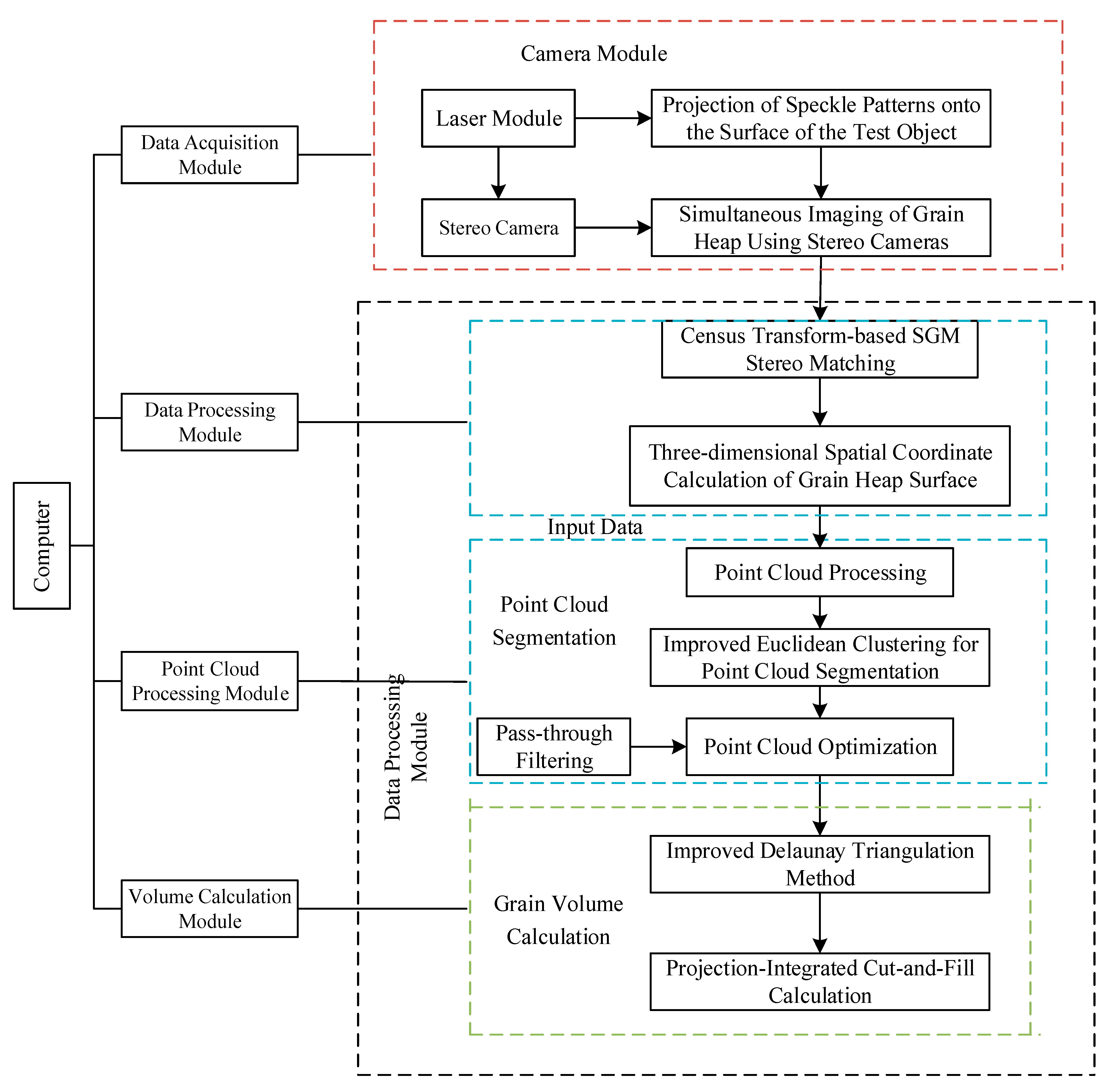
The innovative research contents of this paper are as follows: (1) This paper adopts a binocular structured light reconstruction method based on speckles to address the adverse effects of grain surface texture similarity and uneven illumination on image matching. (2) To achieve effective segmentation of grain pile point cloud images, this paper proposes a fusion of the improved European cluster segmentation method and the through-filter method. (3) This paper establishes a three-dimensional reconstruction system of the grain pile surface and verifies the accuracy of the three-dimensional reconstruction through experiments. (4) The paper utilizes the improved Delaunay method to divide the grain pile point cloud and proposes a volume calculation method based on mesh cuts and complements to achieve accurate measurement of grain pile volume.

The method used in this study to measure the volume of grain piles has the advantage of being non-contact, which means it can calculate the amount of grain by continuously monitoring the volume of the pile. Additionally, it can also provide real-time video monitoring of the grain depot using a vision system without the need for additional hardware. Implementing this technology can greatly simplify the daily inspection and management of grain depots while also reducing the costs associated with inspections for staff.

2. System Construction and Algorithm Implementation

The paper presents the system structure and algorithm implementation diagram, as shown in Figure 1. The modules of the grain pile volume measurement system are primarily divided into four parts: the data acquisition module, data processing module, point cloud processing module, and volume calculation module. The data acquisition module is responsible for projecting structured light onto the surface of the target object, capturing images using a binocular camera, and transmitting these images to a computer. The data processing module includes stereo matching based on a census transform and the acquisition of raw point cloud data. It is used to process the image data transmitted to the computer to obtain raw point cloud data. The point cloud processing module’s primary task is to process and segment the point cloud, which includes improved Euclidean clustering segmentation and pass-through filtering methods. The goal of this module is to transform the raw point cloud data into a point cloud that contains only the grain pile for further operations. The volume calculation module encompasses improved Delaunay triangulation and projection-based segmentation and filling methods. Through these steps, the shape of the grain pile is processed into regular tetrahedrons for the precise calculation of the grain pile’s volume.

3. Binocular Structured Light System

3.1. Experimental Platform

The image acquisition platform in the laboratory is illustrated in Figure 2. In Figure 2a, the capture module comprises a laser module and a binocular camera. The laser module projects the speckle pattern onto the surface of the object being measured and the binocular camera captures images of the object’s surface, as shown in Figure 2b.

The data processing module includes several main steps: firstly, census-transformed semi-global matching (SGM) stereo matching is performed. This step is used to calculate the depth information of the object’s surface and obtain the point cloud information based on the images obtained from the binocular camera. Next, the acquired point cloud of the grain heap is segmented and filtered to accurately extract the valid point cloud of the grain heap, then filtered to remove interference and noise. Finally, the volume of the grain heap is calculated using the processed point cloud data.

The binocular structured light system combines binocular vision and structured light projection techniques. It consists of two cameras and a laser emitter. The laser emitter projects speckle patterns onto the surface of the object being tested, creating a three-dimensional image that reflects the shape of the object’s surface. The binocular cameras capture depth information of the target object’s surface. The first step involves establishing a binocular vision model and calibrating the cameras to obtain their intrinsic and extrinsic parameters. Then, using the principle of similar triangles, the mathematical model of binocular structured light is analyzed to derive the expression for converting disparity to depth. Stereo matching is then performed to calculate the depth information of the object’s surface. By combining the camera’s intrinsic and extrinsic parameters, three-dimensional point cloud data is computed.

3.2. Binocular Camera Model

Binocular vision is a technology that mimics the stereoscopic perception mechanism of the human eye. It achieves this by comparing and merging the visual information captured by binocular cameras to obtain three-dimensional information about objects. In order to explain the relationship between the camera’s imaging plane and the real world [28], as depicted in Figure 3, we will discuss the mapping relationship between coordinate systems.

In the pixel coordinate system, we represent a pixel as $P\left(u\cdot v\right)$, where $u$ and $v$ denote the row and column pixel coordinates, respectively. In the image coordinate system, we denote the image coordinates of point $P$ as $p_L\left(u_L,v_L\right)$ and $p_R\left(u_R,v_R\right)$, corresponding to the pixel coordinates of the left and right cameras, respectively. In the world coordinate system, the coordinates of the point are represented as $P\left(x,y,z\right)$, which indicates the position of a point on the object’s surface in the real world. The rotation matrix, $R$, and translation matrix, $T$, represent the rigid transformation relationship between the coordinate systems of the left and right cameras, i.e., the relative position and orientation between the left and right cameras.

If the physical size of a pixel in the u-axis and v-axis directions is $dx$ and $dy$, respectively, as shown in Figure 4, then the relationship between pixel coordinates and the image plane coordinate system is as follows:

$$\{\begin{array}{c}\begin{array}{c}u=\frac{x}{dx}+u_0\\ v=\frac{y}{dy}+v_0\end{array}\end{array},$$

(1)

Therefore, according to Equation (1), we can deduce:

$$\left[\begin{array}{c}u\\ v\\ 1\end{array}\right]=\left[\begin{array}{ccc}\frac{1}{dx}& 0& u_0\\ 0& \frac{1}{dy}& v_0\\ 0& 0& 1\end{array}\right]\left[\begin{array}{c}x\\ y\\ 1\end{array}\right],$$

(2)

The camera’s intrinsic parameters are as follows:

$$K=\left[\begin{array}{ccc}{f}_x& s& u_0\\ 0& f_y& {\nu }_0\\ 0& 0& 1\end{array}\right],$$

(3)

The effective focal lengths of u and v correspond to $f_x$ and $f_y$ in the intrinsic parameter matrix, respectively. $u_0$ and ${\nu }_0$ represent the offsets of the camera’s optical axis in the image coordinate system. The non-perpendicular factor for $u$ and $v$ is denoted as $S$, which is generally equal to 0.

$R$ is the rotation matrix and $T$ is the translation matrix:

$$R=\left[\begin{array}{ccc}{r}_1& r_2& r_3\\ r_4& r_5& r_6\\ r_7& r_8& r_9\end{array}\right],$$

(4)

$$T=\left[\begin{array}{c}{t}_x\\ t_y\\ t_z\end{array}\right],$$

(5)

The coordinates of point $P$ in the left and right coordinate systems are $\left(x_L,y_L,z_L\right)$ and $\left(x_R,y_R,z_R\right)$, respectively. According to the camera pinhole imaging principle [28], the correspondence between the real-world coordinate system and the camera coordinate system is as follows:

$$z_L\left[\begin{array}{c}{u}_L\\ {\nu }_L\\ 1\end{array}\right]=\left[\begin{array}{ccc}{f}_{Lx}& 0& u_{0L}\\ 0& f_{Ly}& {\nu }_{0L}\\ 0& 0& 1\end{array}\right]\left[\begin{array}{c}{x}_L\\ y_L\\ z_L\end{array}\right],$$

(6)

$$z_R\left[\begin{array}{c}{u}_R\\ {\nu }_R\\ 1\end{array}\right]=\left[\begin{array}{ccc}{f}_{Rx}& 0& u_{0R}\\ 0& f_{Ry}& {\nu }_{0R}\\ 0& 0& 1\end{array}\right]\left[\begin{array}{c}{x}_R\\ y_R\\ z_R\end{array}\right],$$

(7)

where $f_{Lx}$, $f_{Ly}$, $f_{Rx}$, and $f_{Ry}$ are the focal lengths of the left and right camera lenses in the $x$ and $y$ directions on the image plane, respectively. $u_{0L}$, ${\nu }_{0L}$, $u_{0R}$, and ${\nu }_{0R}$ represent the offsets of the camera’s optical axis in the image coordinate system.

According to the rotation matrix and translation matrix, the transformation of point $P$ in the left and right cameras is as follows:

$$\left[\begin{array}{c}{x}_R\\ y_R\\ z_R\end{array}\right]=R\left[\begin{array}{c}{x}_L\\ y_L\\ z_2\end{array}\right]+T,$$

(8)

3.3. Camera Calibration

The calibration of a binocular camera can be divided into intrinsic calibration and extrinsic calibration for the left and right cameras. The goal of extrinsic calibration is to determine the rotation and translation relationship between the two cameras [29,30]. When calibrating the intrinsic parameters of the binocular camera, the calculations should be performed separately. By using Equations (7) and (8), the following results can be obtained:

$$S\left[\begin{array}{c}u\\ v\\ 1\end{array}\right]=K\left[R,T\right]\left[\begin{array}{c}x\\ y\\ z\end{array}\right]=K\left[r_1,r_2,r_3,T\right]\left[\begin{array}{c}x\\ y\\ 0\\ 1\end{array}\right],$$

(9)

where $S$ is the scale factor, and $r_1$, $r_2$, and $r_3$ are the column vectors of the rotation matrix, R. Using the above formula, we can obtain the homography matrix, $H$.

$$H=K\left[r_1,r_2,T\right],$$

(10)

Here, $H=\left[h_1,h_2,h_3\right]$.

By using Equation (10), we can obtain:

$$\left[h_1,h_2,h_3\right]=\lambda k\left[r_1,r_2,t\right],$$

(11)

Based on Equation (11) and the unit orthogonality of the rotation matrix, $R$, we can deduce:

$$h_1{K}^{-T}{K}^{-1}{h}_2=0,$$

(12)

$$h_1^T{K}^{-T}{K}^{-1}{h}_1=h_2^T{K}^{-T}{K}^{-1}{h}_2,$$

(13)

where $r_1=\lambda K^{-1}{h}_1$,$r_2=\lambda K^{-1}{h}_2$,$r_3=r_1\times r_2$,$t=\lambda K^{-1}{h}_3$. Therefore, at least three images are required to uniquely determine the intrinsic camera parameters.

Considering lens distortion, we introduce tangential distortion, $p$, and radial distortion, $k$ [31,32]:

$$\left[\begin{array}{c}{x}_{td}\\ y_{td}\end{array}\right]=\left[\begin{array}{c}x+2p_{1}xy+p_2\left(r^2+2x^2\right)\\ y+2p_{2}xy+p_1\left(r^2+2y^2\right)\end{array}\right],$$

(14)

$$\left[\begin{array}{c}{x}_{rd}\\ y_{rd}\end{array}\right]=\left(1+k_1{r}^3+k_2{r}^4+k_3{r}^6\right)\left[\begin{array}{c}x\\ y\end{array}\right],$$

(15)

Combining Equations (14) and (15), we obtain the following:

$$\left[\begin{array}{c}{x}_d\\ y_d\end{array}\right]=\left[\begin{array}{c}x\left(1+k_1{r}^3+k_2{r}^4+k_3{r}^6\right)+2p_{1}xy+p_2\left(r^2+2x^2\right)\\ y\left(1+k_1{r}^3+k_2{r}^4+k_3{r}^6\right)+2p_{2}xy+p_1\left(r^2+2y^2\right)\end{array}\right],$$

(16)

After obtaining the intrinsic parameters through calibration, we need to acquire the camera’s extrinsic parameters. Let’s assume a point, $P$, in space with its coordinates represented in the world coordinate system as $P_w$. This point can also be represented in the left and right camera coordinate systems:

$$\{\begin{array}{l}\begin{array}{l}{P}_R=R_R{P}_w+T_R\end{array}\\ P_L=R_L{P}_w+T_L\end{array},$$

(17)

In this case, $R_R$ is the rotation matrix from the left camera to the right camera, $R_L$ is the rotation matrix from the right camera to the left camera, $T_R$ is the translation matrix from the left camera to the right camera, and $T_L$ is the translation vector from the right camera to the left camera. $P_L$ and $P_R$ are the coordinates of point $P$ in the left and right camera coordinate systems.

Assuming the left camera as the main coordinate system and combining Equation (8), we obtain:

$$P_L=R_{RL}{P}_R+T_{RL},$$

(18)

where $R_{RL}$ represents the rotation matrix from the right camera to the left camera and $T_{RL}$ represents the translation vector from the right camera to the left camera.

Based on the rotation matrices $R_R$ and $R_L$, as well as the translation matrices $T_L$ and $T_R$, we can derive:

$$\{\begin{array}{l}{R}_{RL}=R_L{R}_R^{-1}\\ T_{RL}=T_L-R_{RL}{T}_R\end{array},$$

(19)

3.4. Surface Structured Light Model

Traditional binocular vision is highly sensitive to changes in the environment, particularly when the grain piles lack distinct textures. In order to achieve precise 3D reconstruction of grain piles, this study introduces the use of structured light technology based on the speckle method. Structured light technology can effectively increase the number of feature points on the object, enhance texture information, and minimize the impact of weak and repetitive texture regions, thus enabling accurate point correspondence. The working principle of the structured light measurement for surface reconstruction is illustrated in Figure 5. The structured light system comprises a laser module, cameras, and the object surface. The laser module consists of a vertical-cavity surface-emitting laser (VCSEL) array and a beam expander. Both the laser module and the left and right cameras are positioned on the same horizontal line. The laser module projects speckle patterns onto the object surface, which are subsequently captured by the cameras.

For the 3D reconstruction of grain piles, two cameras are placed in parallel to capture the speckle patterns projected by the laser module. The mathematical model for binocular structured light is shown in Figure 6. In this model, point $P$ is a point in the world coordinate system, and $P_1$ and $P_2$ are the corresponding image points of point $P$ on the left and right image planes, respectively. The focal length is represented by $f$, while $O_l$ and $O_r$ are the optical centers of the left and right cameras. The optical axes of the two cameras are parallel. $x_l$ and $x_r$ denote the distances from the two image points to the left edges of their respective image planes.

According to the principle of similar triangles, the following relationships can be derived:

$$\frac{Z}{T}=\frac{Z-f}{T-\left(x_l-D_l\right)-\left(D_r-x_r\right)},$$

(20)

Assuming the left camera as the main coordinate system, the coordinates of point $P$ in space can be expressed as:

$$\{\begin{array}{l}\begin{array}{c}X=Z\frac{x}{f}\end{array}\\ Y=Z\frac{y}{f}\\ Z=\frac{-f\times T}{\left(D_l-D_r\right)-\left(x_l-x_r\right)}\end{array},$$

(21)

where $Z$ and $f$ represent the depth of point $P$ and the camera’s focal length, respectively. $\left(x_l-D_l\right)$ is the distance between two points and $\left(D_r-x_r\right)$ is the distance between two points. $T$ is the baseline distance, where $\left(x_l-x_r\right)-\left(D_l-D_r\right)$ is the disparity, which is the difference between the corresponding points of the same 3D point in the left camera’s pixel and the right camera.

4. Stereo-Matching Algorithm

In this paper, we utilize speckle structured light in combination with the semi-global stereo matching algorithm to enhance texture information and compute disparity values. The semi-global stereo matching algorithm is a widely used technique that combines the advantages of global matching and local block matching, resulting in improved matching accuracy while maintaining global consistency. Traditional matching cost computation relies on mutual information theory [33], which requires initial disparity values and necessitates layered iterations to obtain more precise matching cost values. However, this approach involves complex probability distribution calculations, leading to inefficiencies in cost computation. Additionally, mutual information theory is sensitive when dealing with cases that have weak textures and significant lighting variations.

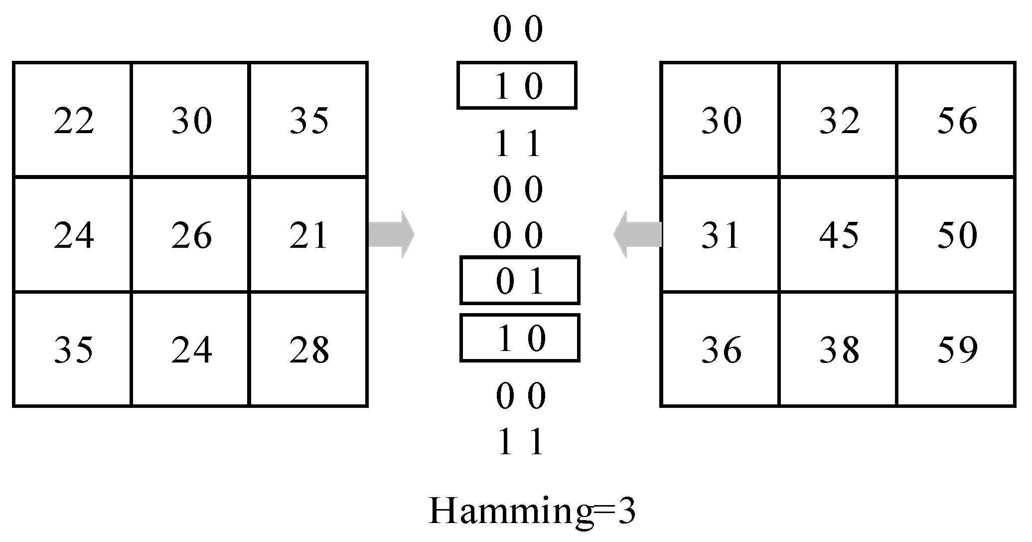
The census transform [34] generates a code by comparing the relative relationships between a pixel and its surrounding neighboring pixels. This property allows the census transform to handle lighting variations and noise in images more effectively. Moreover, the census transform operates within a local window, which enhances its parallelism.

To compute the matching cost, we utilize the census transform to calculate the initial cost. The process of census transformation is depicted in Figure 7. By setting a window of size $b\times b$, we use the pixel intensity difference with respect to the central pixel’s intensity value as a reference to compare other pixels within the window. The result of the census transform is the generation of a bit string, and the census transform value is given by:

$$C_c\left(u,v\right)=\stackrel{n^{\prime }}{\underset{i=-n}{\otimes }}\stackrel{m^{\prime }}{\underset{j=-m}{\otimes }}\zeta \left(I\left(u,v\right),I\left(u+i,v+j\right)\right),$$

(22)

where $\otimes$ represents bitwise operation and $n^{\prime }$ and $m^{\prime }$ are the largest integers not exceeding half of $n$ and $m$, respectively. The $\zeta$ operation is defined as follows:

$$\zeta \left(x,y\right)=\{\begin{array}{l}\begin{array}{l}0,\hspace{1em}ifx\le y\\ 1,\hspace{1em}other\end{array}\end{array},$$

(23)

The matching cost for census transformation is computed as the $Hamming$ distance between the output bit strings:

$$C\left(n,v,d\right)=Hamming\left(C_L\left(n,\nu \right),C_R\left(u-d,v\right)\right),$$

(24)

where $C_L$ and $C_R$ represent the bit strings in the left and right images.

The initial cost computation does not take into account the disparity similarity constraint, which can lead to a significant number of noise points. To overcome this issue, the initial cost is refined through cost aggregation and the matching cost is constrained by cost propagation. To achieve cost aggregation and constraint implementation, we designed a global energy function, $E\left(D\right)$, in this study. The purpose of cost aggregation is to improve the initial cost by taking into account the disparity relationships in the neighborhood of matching points. This helps in obtaining an optimization strategy for the global energy function. When the disparity value of a pixel point reaches its optimal value, the energy function achieves its minimum value.

The energy function, $E\left(D\right)$, is defined as follows:

$$E\left(D\right)={\sum }_p(C\left(p,D_p\right)+{\sum }_{q\in N_p}{P}_{1}T\left[\left|D_p-D_q\right|=1\right]+{\sum }_{q\in N_p}{P}_{2}T\left[\left|D_p-D_q\right|>1\right]),$$

(25)

where $D_p$ represents the disparity of pixel point $p$, $P_1$ and $P_2$ are penalty parameters, $C\left(p,D_p\right)$ is the initial cost at pixel point $p$ for disparity $D_p$, and $N$ represents the neighborhood of pixel points.

${\sum }_{p}C\left(p,D_p\right)$ is the summation of matching costs for all pixels in the disparity map, $D$.${\sum }_{q\in N_p}{P}_{1}T\left[\left|D_p-D_q\right|=1\right]$ represents the constant penalty value, $P_1$, added when the disparity difference between pixel $p$ and its neighboring pixel, $q$, is 1. Similarly,${\sum }_{q\in N_p}{P}_{2}T\left[\left|D_p-D_q\right|>1\right]$ adds a larger penalty value, $P_2$, for larger disparity differences. The global energy function requires accumulating the matching costs for all pixels in the disparity map and introducing penalty values to constrain the matching results. Small penalty values can adapt to slanted and curved surfaces, while larger penalty values are suitable for depth discontinuity regions. Depth discontinuities typically occur at locations with significant grayscale changes, so $P_2$ is determined adaptively based on the grayscale gradient:

$$P_2=\frac{P_2^{\prime }}{\left|I_{bp}-I_{bq}\right|},$$

(26)

where $P_2^{\prime }$ is a fixed value and $I_{bp}$ and $I_{bq}$ represent the grayscale values of the current pixel point and the surrounding pixel points along the same path as the current pixel point.

SGM aggregates matching costs from various directions to reduce the impact of errors and obtain an optimal energy function. The cost for pixel $p$ at disparity $d$ is recursively defined as follows:

$$L_r\left(p,d\right)=C\left(p,d\right)+min\left(\begin{array}{c}{L}_r\left(p-r,d\right)\\ L_r\left(p-r,d-1\right)+P_1\\ L_r\left(p-r,d+1\right)+P_1\\ \underset{i}{min}{L}_r\left(p-r,i\right)+P_2\end{array}\right)-\underset{i}{min}{L}_r\left(p-r,i\right),$$

(27)

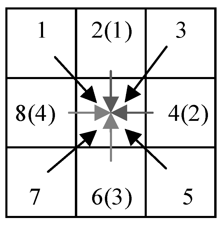
where $r$ represents a path, $p-r$ denotes the pixels along that path preceding pixel $p$, and $L_r\left(p,d\right)$ refers to the matching cost when the pixel $p$ has a disparity value of $d$ along the path, $r$. The semi-global stereo matching algorithm seeks to find the minimum aggregated cost from various directions, and the final aggregated cost is the sum of the aggregated costs along all paths:

$$S\left(p,d\right)={\sum }_r{L}_r\left(p,d\right),$$

(28)

The path aggregation is illustrated in Figure 8, where eight directions are aggregated for each pixel. This process yields the corresponding energy functions. In Figure 8, there are two path aggregation methods: 4-path aggregation (light-colored arrows) and 8-path aggregation (black + light-colored arrows).

After cost aggregation, to further improve the stereo matching accuracy, the winner takes all (WTA) method is employed to calculate the disparity. In the WTA method, the pixel with the minimum matching cost is selected, and its corresponding disparity value becomes the optimal disparity. The initial disparity calculation is given by:

$$d^{*}=argminS\left(p,d\right),$$

(29)

where $d^{*}$ represents the disparity value of the pixel at position $p$ and $S\left(p,d\right)$ denotes the aggregated cost value.

Disparity optimization aims to enhance the accuracy of the disparity map by eliminating incorrect disparities. In this study, the left–right consistency check is used, which is based on the uniqueness constraint of disparity. By comparing the disparity maps of the left and right images, disparities that do not meet the uniqueness constraint are eliminated, resulting in improved depth information accuracy. The formula for the consistency check is:

$$D_p=\{\begin{array}{cc}{D}_{bp}& if\left|D_{bq}-D_{mq}\right|\le 1\\ D_{invalid}& otherwise\end{array},$$

(30)

After the disparity optimization, a more reliable disparity map is obtained, providing a solid foundation for obtaining the point cloud of the grain pile and conducting volume measurements.

5. Data Acquisition

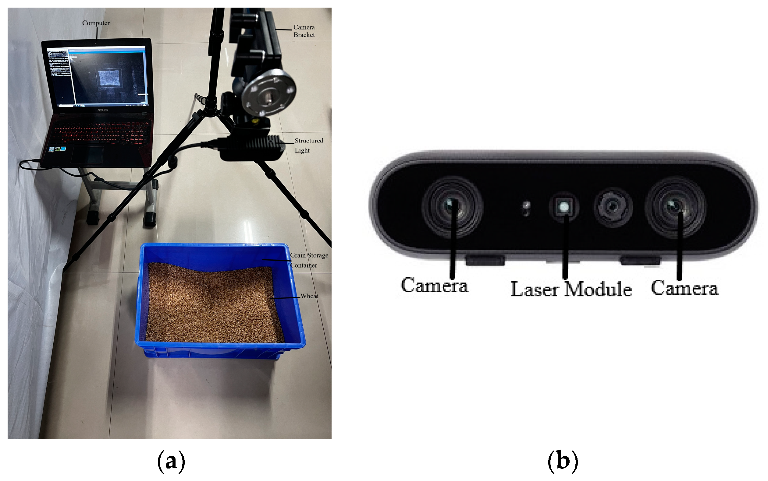
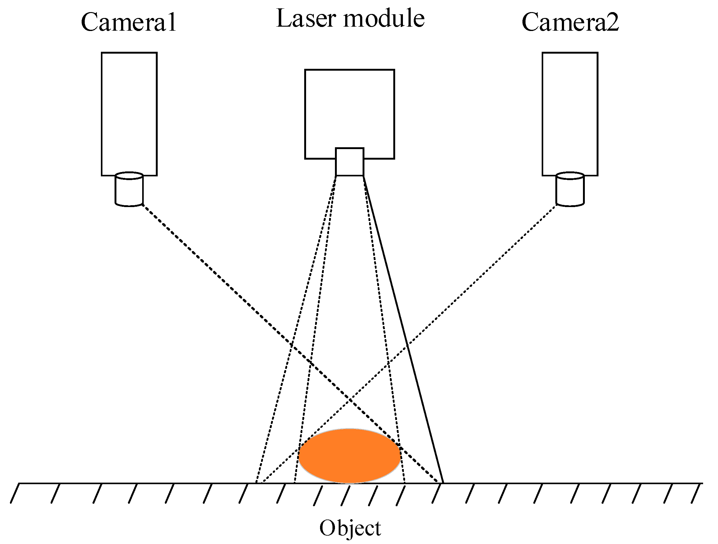
The hardware platform for surface 3D reconstruction of the grain pile primarily includes a display, a workstation (CPU: i5-12400F, GPU: 2060s), a binocular structured light system, and a camera mount. The binocular structured light system consists of two cameras and a laser emitter. The height of the binocular structured light can be adjusted by modifying the height of the camera mount.

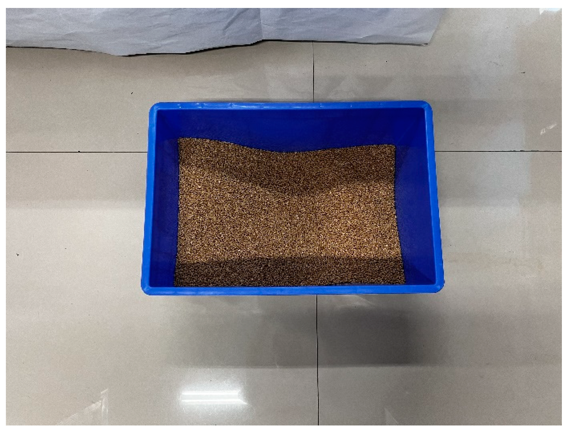
This study focuses on the Zhengmai 22 wheat variety from Kaifeng, Henan Province, China. Based on the storage characteristics, a grain storage model is constructed as shown in Figure 9. The grain storage container is a lidless rectangular box with dimensions of 520 mm × 355 mm × 285 mm. The true volume is measured to be 0.019 m³ using the drainage method. Different shapes of wheat grain piles are constructed in the storage container as shown in

Table 1. Experiments with different grain pile surface areas.

Number of Grain Pile Type	Grain Heap Shape
1	Grain heap flattening
2	Grain heap tilted left
3	Grain heap tilted right
4	Grain heap convex in the middle
5	Grain heap concave in the middle
6	The grain pile did not fully cover the container

. In order to investigate the impact of various grain pile shapes on volume measurement, this study aims to verify the stability and applicability of the measurement system. To simulate real-world grain warehouse storage conditions, different grain pile shapes were created, and experiments were conducted.

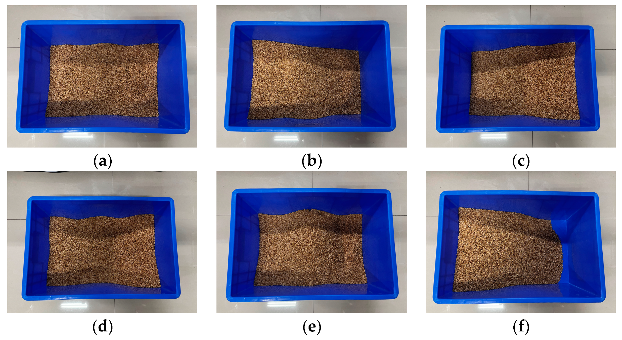
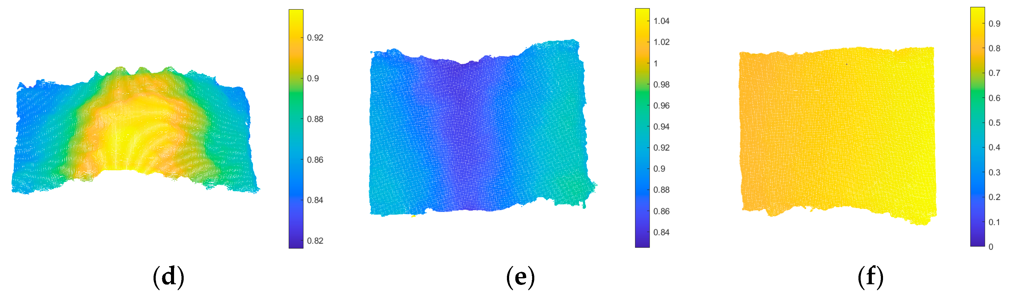
In Figure 10a, a grain pile is shown with a flattened surface to achieve a smooth and even shape. Figure 10b depicts a grain pile with a surface tilted to the left, forming an inclined shape. Similarly, Figure 10c showcases a grain pile with a right tilt, creating another inclined shape. Figure 10d displays the raised middle part of a grain pile surface, which results in a protruding shape. In Figure 10e, the middle part of the grain pile is depressed, which produces a concave shape. Lastly, Figure 10f presents a grain pile model that does not completely cover the container.

With these different grain pile shapes, volume measurement experiments are conducted to understand the influence of shape on the measurement results. This research provides important practical value for grain storage and related fields. The grain pile model we have developed takes into account the practical application background and is designed to be compatible with the actual situation of grain warehouse storage. It also possesses universality.

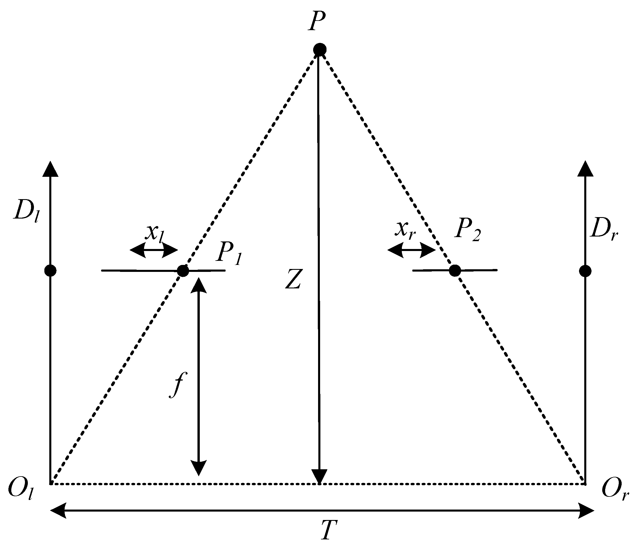
Using the binocular structured light system constructed in this study, we conducted measurements on simulated wheat grain storage. We also established a point cloud acquisition method for the grain pile based on stereo matching algorithms. The binocular structured light system captures images, and the disparity values of the grain pile images are extracted using a stereo matching algorithm that is based on the minimum energy cost function. By combining the binocular structured light mathematical model, the disparity map is converted into a depth map. With the assistance of the binocular vision model and calibration parameters, the depth map is transformed into a point cloud, allowing for the achievement of 3D reconstruction of the grain pile.

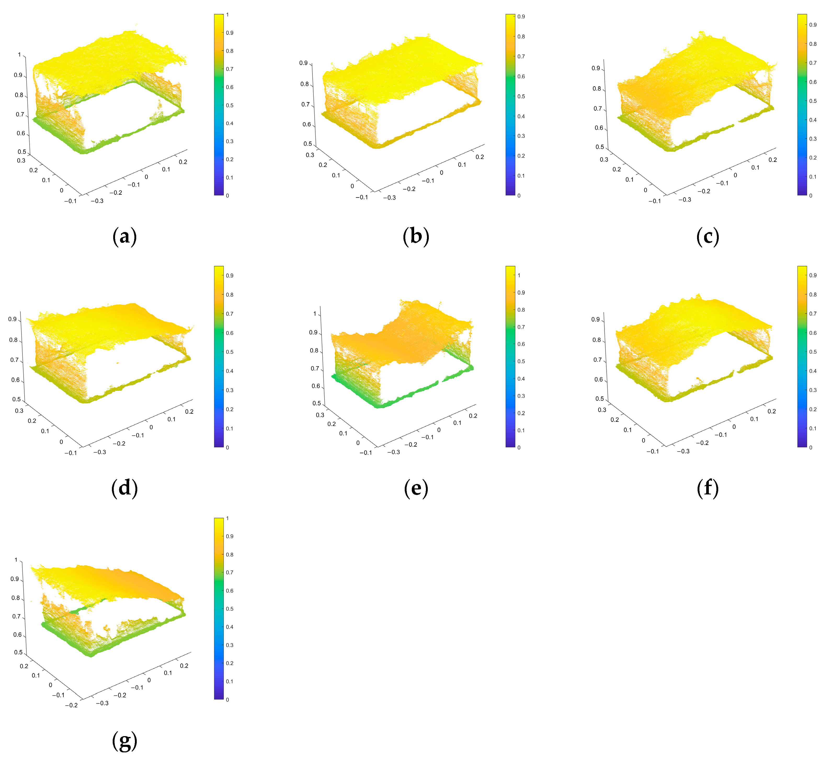
The acquired image information is converted into a depth map using stereo matching and a binocular structured light model. By utilizing camera calibration parameters and a binocular vision model, the depth map can be further transformed into point cloud data. The resulting point cloud data is then analyzed, as shown in Figure 11. Figure 11a represents the point cloud data without the grain pile, while Figure 11b–g depict the point cloud data with various configurations of the grain pile, such as being flat, left-leaning, right-leaning, convex, concave, or not completely covering the bottom of the container.

5.1. Improving Point Cloud Segmentation Using Enhanced Euclidean Clustering

According to Figure 11, the point cloud data obtained includes not only the point cloud of the grain pile but also the point cloud of the storage container. In order to accurately measure the volume of the grain pile, it is important to effectively separate the point cloud of the grain pile from the overall point cloud through segmentation during the subsequent analysis.

Currently, point cloud segmentation includes fitting-based point cloud segmentation, clustering-based point cloud segmentation, and deep learning-based point cloud segmentation. Li et al. [35] proposed an improved RANSAC (random sample consensus) method based on normal distribution transformation units to avoid false plane segmentation in 3D point clouds. The method’s reliability and applicability were demonstrated through experiments, with correctness exceeding 88.5% and completeness exceeding 85.0%. Isa et al. [36] used RANSAC and localization methods to segment 3D point cloud data acquired from ground-based LIDAR scans, and the method was tested on a clock tower, showing the capability to perform proper segmentation of the data. Li et al. [37] introduced a multi-primitive reconstruction (MPR) method, which first segments primitives through a two-step RANSAC strategy, followed by global primitive fitting and 3D Boolean operations. Experimental results verified the effectiveness of the proposed method. However, these methods have certain limitations in segmenting irregular objects, especially when RANSAC algorithms are typically used for regular point cloud segmentation, such as lines, planes, spheres, etc. They may perform poorly for segmenting irregular objects. Although RANSAC algorithms can be applied to irregular object segmentation in certain cases, they often require combination with other algorithms or techniques to handle complex geometries and features to achieve more accurate and robust segmentation results.

Cluster-based point cloud segmentation divides the point cloud into different clusters to achieve object segmentation. Miao et al. [38] proposed a single plant segmentation method based on Euclidean clustering and K-means clustering. The results showed that this method can address the issue of Euclidean clustering failing to segment cross-leaf plants. Chen et al. [39] modified the classical DBSCAN clustering algorithm for 3D point cloud boundary detection and plane segmentation. They performed plane fitting and validity detection based on candidate samples in 3D space. Xu et al. [40] used statistical filtering based on Gaussian distribution to remove outlier points, followed by an improved density clustering algorithm for coarse point cloud segmentation. They further addressed over-segmentation and under-segmentation issues using normal vectors for segmentation. The experimental results showed the effectiveness of their proposed method. However, it is worth noting that cluster-based methods usually involve manual parameter selection, including the number of clusters and distance metric methods. These parameter choices can have a significant impact on the segmentation results, often requiring experience or multiple attempts to achieve better outcomes. Furthermore, traditional cluster-based methods often prioritize geometric or attribute features of the data while neglecting semantic information. In certain applications, point cloud segmentation needs to consider object semantic relationships and contextual information, as they are crucial for achieving more accurate results. Deep learning-based point cloud segmentation is currently a widely used method. However, it encounters challenges such as the need for large amounts of data, extensive annotation for training, and the requirement for powerful computing resources. Moreover, deep learning-based methods for irregular point cloud segmentation require further research and improvement.

Considering the irregularity and continuity of grain surface point clouds, as shown in Figure 11, which depicts the target scene that includes not only the grain pile surface but also the container, it is necessary to extract valid point clouds of the grain pile for further calculations. This study proposes an improved Euclidean clustering point cloud segmentation method. This method sets seed points in the point cloud and divides the point cloud into different categories based on Euclidean distance to achieve segmentation of the grain pile point cloud. Compared to traditional Euclidean clustering methods, as shown in Figure 12, which have difficulties accurately segmenting the required grain pile point cloud, the proposed method not only considers the spatial features of the point cloud but also the continuity between different categories, resulting in more accurate and robust segmentation results.

In order to optimize the improved Euclidean clustering segmentation method and improve computational efficiency, this paper adopts a parallel computing strategy and combines it with the direct pass filter to eliminate outliers. The segmentation is performed on two sets of point clouds, where set $P_2$ represents the point cloud without grain heap data and set $P_1$ contains the point cloud with the grain heap. The specific steps are as follows:

Step 1: Select $p_{21}$ as the seed point in $P_2$ and calculate the Euclidean distances to find the closest points in set $P_1$. Then, based on the set threshold, determine if the distance between the point and $p_{21}$ is smaller than the threshold. If it meets the condition, add the point to class $Q$.

Step 2: Continue selecting new seed points and repeat step 1 until no new points are added to class $Q$.

Step 3: Point set $P_1$ contains the effective point cloud of the grain heap and set $Q$ contains the point cloud that does not belong to the grain heap. Therefore, point set $Q$ can be removed from point set $P_1$ to obtain the final point cloud of the grain heap.

This paper takes into consideration the irregularity and disorderliness of the grain heap point cloud, as well as the subsequent operations and economic benefits. While traditional point cloud segmentation methods usually focus on segmenting different parts from the point cloud data, the objective of this paper is to obtain the point cloud of the grain heap for volume calculation. To achieve this, two sets of point cloud data are utilized and classified based on Euclidean distance. As shown in Figure 11, Figure 11a represents the point cloud without the grain heap, Figure 11b represents the point cloud with a flat grain heap, Figure 11c with a left-leaning grain heap, Figure 11d with a right-leaning grain heap, Figure 11e with a convex grain heap, and Figure 11f with a concave grain heap. Additionally, Figure 11g shows point clouds where the grain pile does not fully cover the container. These point clouds include those containing only the container and those containing both the container and the grain heap. Figure 11b–g are combined with the Figure 11a point cloud, and then a distance threshold is set to calculate the distance from each point in the point cloud to its nearest neighbor point. The point cloud data is then filtered based on this threshold.

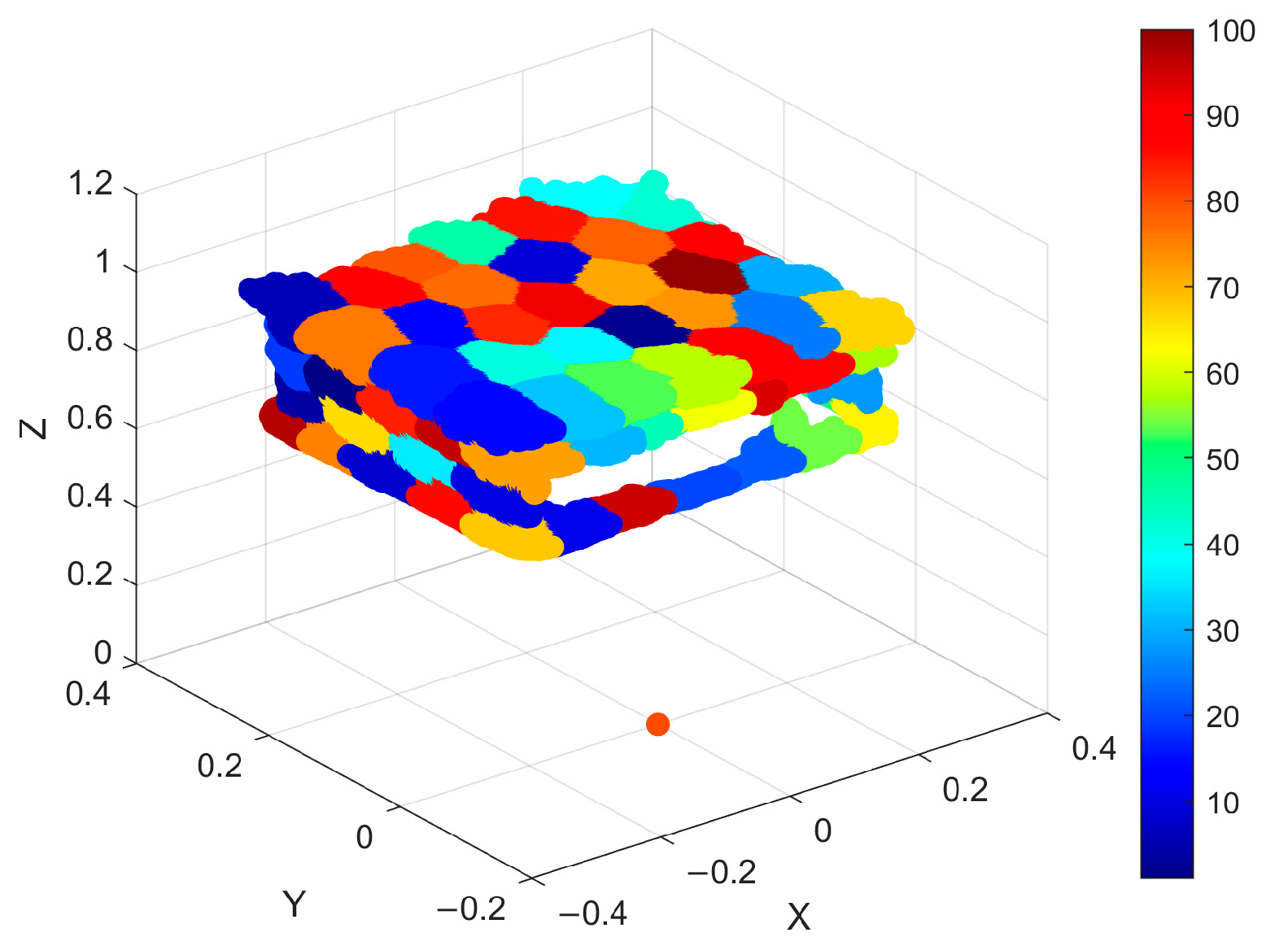
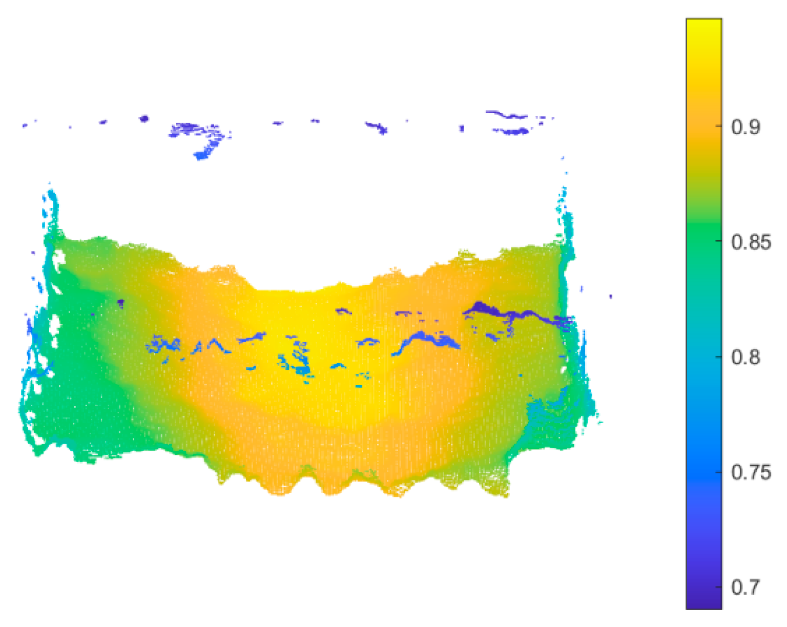
Figure 13 illustrates a set of point clouds that were generated using the point cloud segmentation method proposed in this paper. Upon examining the results depicted in the figure, it becomes apparent that the proposed segmentation method successfully and accurately separates the grain heap information from the entire point cloud. The grain heap point cloud demonstrates specific height and shape characteristics.

Considering the situation where the computation is computationally intensive, this paper adopts parallel computing to decompose the task into multiple sub-tasks and processes them simultaneously, greatly accelerating the overall processing speed. Unlike traditional point cloud segmentation methods, this paper does not use downsampling to reduce the number of point clouds but employs more efficient parallel computing to maintain the point cloud density and texture details while maximizing the efficiency of subsequent calculations. This improved approach preserves the density and texture details of the point cloud while significantly increasing the speed of point cloud processing, making it more suitable for engineering practical needs such as grain heap volume calculation. By considering the characteristics of grain heap point clouds of different shapes and utilizing parallel computing techniques, this paper provides an efficient and accurate point cloud processing method for grain storage and related fields, which is of great significance for improving engineering efficiency and economic benefits.

5.2. Grain Pile Point Cloud Optimization

The pass-through filter is a widely used method in point cloud filtering. It effectively removes points from the point cloud that fall outside a specified range along a given coordinate axis. This filter is particularly useful in eliminating outliers and filtering out points that are beyond the specified range. By doing so, it improves the accuracy and reliability of the point cloud data by reducing interference. In the context of grain heap point cloud segmentation, the pass-through filter is employed to eliminate outliers and poorly segmented boundary points from the point cloud.

As depicted in Figure 13, the point cloud of the segmented grain heap surface contains outliers and poorly segmented boundary points, which could be noise or a result of imperfect segmentation algorithms. In order to enhance the accuracy and reliability of the point cloud data, this study employs the pass-through filter. This filter efficiently eliminates outliers and filters out poorly segmented points along the boundary. The steps involved in the pass-through filtering process are as follows:

(1)

Select the point cloud axis to be retained: First, it is necessary to choose the coordinate axis (e.g., x, y, z) to be retained based on the characteristics of the point cloud data.

(2)

Specify the range along the selected axis: Next, specify the minimum and maximum values along the selected axis to be retained. Points outside this range will be filtered out, effectively removing outliers.

(3)

Execute the filtering: Based on the specified range, execute the pass-through filtering, retaining the points within the specified range and removing points outside the range. This process effectively eliminates outliers and poorly segmented points, resulting in a cleaner and more accurate grain heap surface point cloud.

Comparing Figure 13 and Figure 14, the pass-through filter effectively removes unnecessary point cloud data and improves the accuracy and reliability of point cloud segmentation. This processing step provides a more reliable foundation for subsequent grain heap volume calculations. The use of the pass-through filter in this study successfully enhances the quality of grain heap surface point cloud data, providing more accurate data support for research and applications in grain storage domains.

By comparing the results in Figure 14 with those in Figure 11 and Figure 13, it is evident that the improved Euclidean clustering point cloud segmentation combined with the pass-through filter effectively and accurately separates the grain heap point cloud information from the entire point cloud. This process eliminates interference points and outliers, enhancing the quality and accuracy of the point cloud data. In Figure 15, the successful segmentation of the grain heap point cloud can be observed while irrelevant points, such as the container, are filtered out. The application of the improved Euclidean clustering point cloud segmentation method combined with the pass-through filter improves the efficiency, accuracy, and reliability of the segmentation process for the grain heap point cloud. This method considers the spatial characteristics of the point cloud and the continuity between different categories, resulting in more accurate and robust segmentation. Furthermore, the use of the pass-through filter removes unnecessary point cloud data, thereby improving the quality of the point cloud data.

6. Volume Calculation

Currently, various methods exist for calculating volume based on point clouds, such as the convex hull method, the slicing method, the model reconstruction method, and the projection method. In this paper, we introduce a volume calculation method that combines mesh patching with the projection method. The underlying principle is to divide the 3D point cloud into a triangular mesh structure, project the mesh downwards, and generate multiple irregular triangular prisms. The volumes of these irregular triangular prisms are then calculated and summed to obtain the total volume. Although there is currently no direct method for calculating the volume of irregular triangular prisms, they can be decomposed into a regular triangular prism and a triangular or quadrangular pyramid through mesh patching. Our proposed method, in comparison to the methods proposed by Wang et al. [41] and Zhang et al. [10], which utilize the average elevation or average depth of all points in the mesh as the height, achieves smaller errors in volume calculation. The primary source of errors lies in the mesh partitioning.

Delaunay triangulation is a reliable and stable meshing method that preserves the topological properties of point cloud data. This method helps to retain the geometric features of the point cloud and generate a continuous and non-overlapping triangular mesh. It possesses the properties of an empty circle and maximizes the minimum angle. The empty circle property ensures that no four points in the triangular mesh share a circle, and the circumcircle of any triangle does not contain other points, ensuring the stability and consistency of the triangles. The maximization of the minimum angle property ensures that the generated triangles have large minimum angles, thereby improving the quality of the triangular mesh. Larger minimum angles help reduce sharp angles and distortions, resulting in more uniform and regular triangles. Furthermore, regardless of the angle at which the construction starts, the final result remains consistent.

This paper presents an improved Delaunay triangulation method that addresses the issues of inconsistent or incomplete triangle shapes and elongated triangles in traditional Delaunay triangulation. These issues often arise due to interruptions or incompleteness in the point set. To overcome these challenges, we propose the introduction of a distance threshold to control the maximum edge length of the generated triangles in the traditional Delaunay triangulation method. By incorporating this distance threshold, our method ensures that the triangles on the boundary of the point cloud remain consistent and well-formed while minimizing the occurrence of elongated triangles. This refinement significantly improves the accuracy of subsequent volume calculations, making our method more suitable for handling point clouds with boundary interruptions or incompleteness. The proposed method consists of the following steps:

(1) Firstly, a point is selected from the point set and used as the center of a circle. Then, points within the threshold range from the center of the circle are searched for. One of the scattered points is chosen and connected to the center point to generate an initial edge length. If no points are found within the threshold range, the process is repeated until all points in the point set have been used.

(2) Once the initial edge length is determined, scattered points around it are searched for. A point is considered to be part of an initial triangle if its distance to one endpoint of the edge is smaller than the threshold.

(3) The initial triangle’s edges are then used as the ‘to-be-expanded’ edges. The triangle is expanded based on the threshold, with the requirement that the scattered points are located on the two sides of the ‘to-be-expanded’ edge. If no points are found within the threshold range, step (1) is repeated.

(4) Calculate the angle between the normal vectors of the ‘to-be-expanded’ triangle and the expanded triangle. Select the triangle with the largest angle as the expanded triangle.

(5) If there are multiple triangles that meet the conditions in step (4), compare the minimum angles of the triangles and choose the triangle with the largest minimum angle as the expanded triangle. Repeat this process until all points have been selected. End the process.

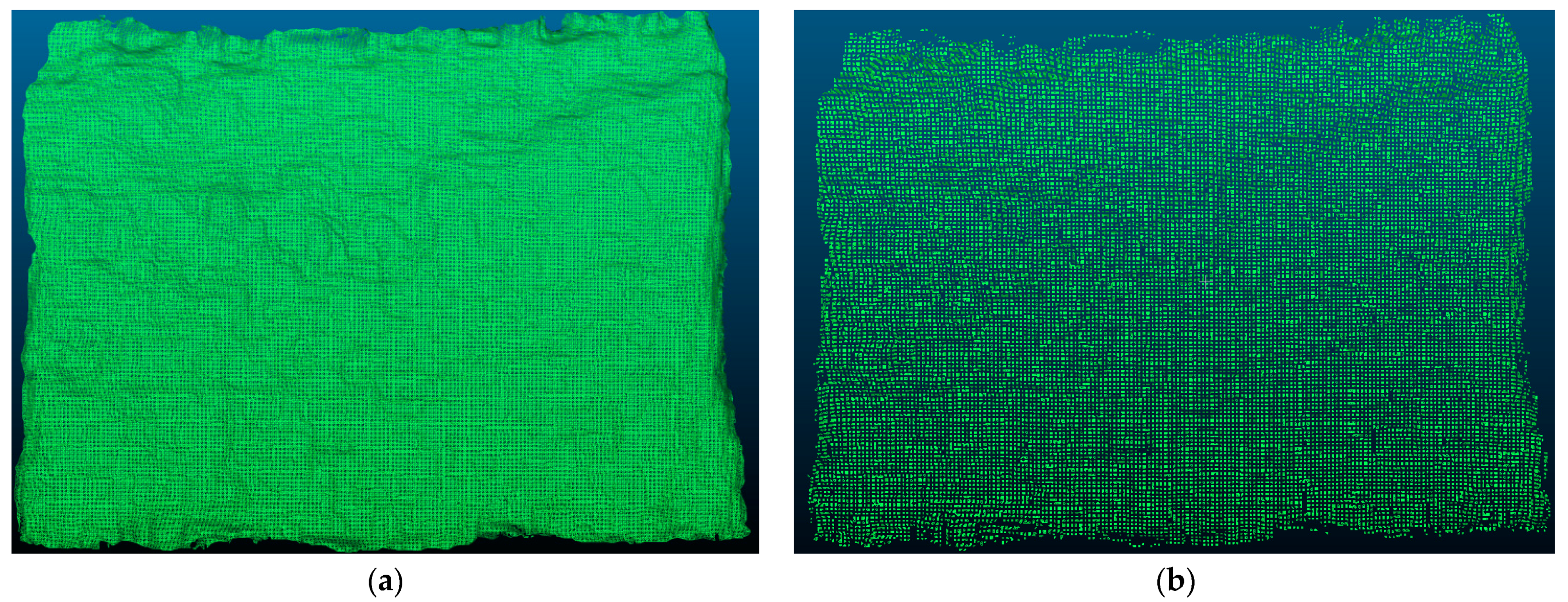
Figure 15 shows the segmentation results obtained using different thresholds (2 mm and 5 mm). From the figures, it is evident that when the threshold is set too small (2 mm), numerous holes appear, indicating the presence of small triangles that form disjointed regions. However, as the threshold is increased to 5 mm, the number of holes decreases and the point cloud data becomes more continuous, thereby better preserving the shape of the grain heap. Therefore, in practical applications, selecting an appropriate threshold is crucial to ensure accurate and continuous segmentation of the point cloud. This improved Delaunay triangulation method provides more reliable and accurate foundational data support for subsequent calculations of grain heap volume.

In this study, the true volume of the grain heap was measured to be 0.019 m³ using the drainage method. To validate the stability of the structured light system, measurements were conducted for six different shapes of grain heaps (flat, left-leaning, right-leaning, concave, convex, and the grain pile does not fully cover the container.). After obtaining the point cloud data, segmentation was performed, followed by the application of the improved Delaunay triangulation to triangulate the point cloud. The volume of the grain heap was then obtained using a combination of the projection method and the cut-and-fill method.

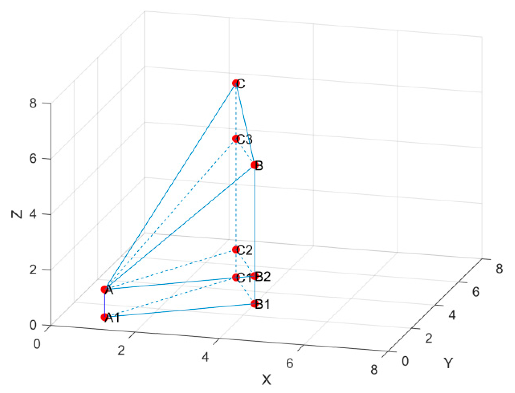
As shown in Figure 16, A, B, and C represent a triangular face after triangulation. When projecting triangle ABC onto the xoy-plane, it forms an irregular triangular prism, $BC-A_1{B}_1{C}_1$. This irregular triangular prism can be further divided into a regular triangular prism, $A{B}_2{C}_2-A_1{B}_1{C}_1$, a four-sided pyramid, $A-B{B}_2{C}_2{C}_3$, and a triangular pyramid, $A-BC{C}_3$. The volume of this irregular triangular prism, $ABC-A_1{B}_1{C}_1$, can be represented as follows:

$$V_{ABC-A_1{B}_1{C}_1}=V_{A{B}_2{C}_2-A_1{B}_1{C}_1}+V_{A-B{B}_2{C}_2{C}_3}+V_{A-BC{C}_3}$$

(31)

$$\{\begin{array}{l}\begin{array}{l}{V}_{A{B}_2{C}_2-A_1{B}_1{C}_1}=S_{\Delta A_1{B}_1{C}_1}\times h_1\\ V_{A-B{B}_2{C}_2{C}_3}=\frac{1}{3}{S}_{B{B}_2{C}_2{C}_3}\times h_2\\ V_{A-BC{C}_3}=\frac{1}{3}{S}_{BC{C}_3}\times h_3\end{array}\end{array}$$

(32)

Based on the information presented in Figure 16, we conducted a projection of the subdivided space triangle to obtain an irregular triangular prism. By analyzing the point cloud data, we were able to determine the three-dimensional coordinates of the triangle’s vertices. Through further calculations, we obtained the necessary height measurements for calculating the volume of each triangular prism. Formula 2 in the paper introduces three height values. In this scenario, let ${\mathrm{h}}_1$ represent the height of the triangular prism ${\mathrm{AB}}_2{\mathrm{C}}_2-{\mathrm{A}}_1{\mathrm{B}}_1{\mathrm{C}}_1$. The ${\mathrm{z}}_{\mathrm{A}}$ value corresponds to the z-axis coordinate of point A. Additionally, ${\mathrm{h}}_2$ denotes the distance between points A and ${\mathrm{B}}_2{\mathrm{C}}_2$, which signifies the height of the triangular pyramid $\mathrm{A}-{\mathrm{BB}}_2{\mathrm{C}}_2{\mathrm{C}}_3$. Similarly, ${\mathrm{h}}_3$ represents the distance between points A and ${\mathrm{B}}_2{\mathrm{C}}_2$, indicating the height of the triangular pyramid $\mathrm{A}-{\mathrm{BCC}}_3$.

The volume of the grain pile is:

$$V={\sum }_1^n{V}_n$$

(33)

where $n$ represents the number of irregular prisms and $V_n$ denotes the volume of the irregular prism with index $n$.

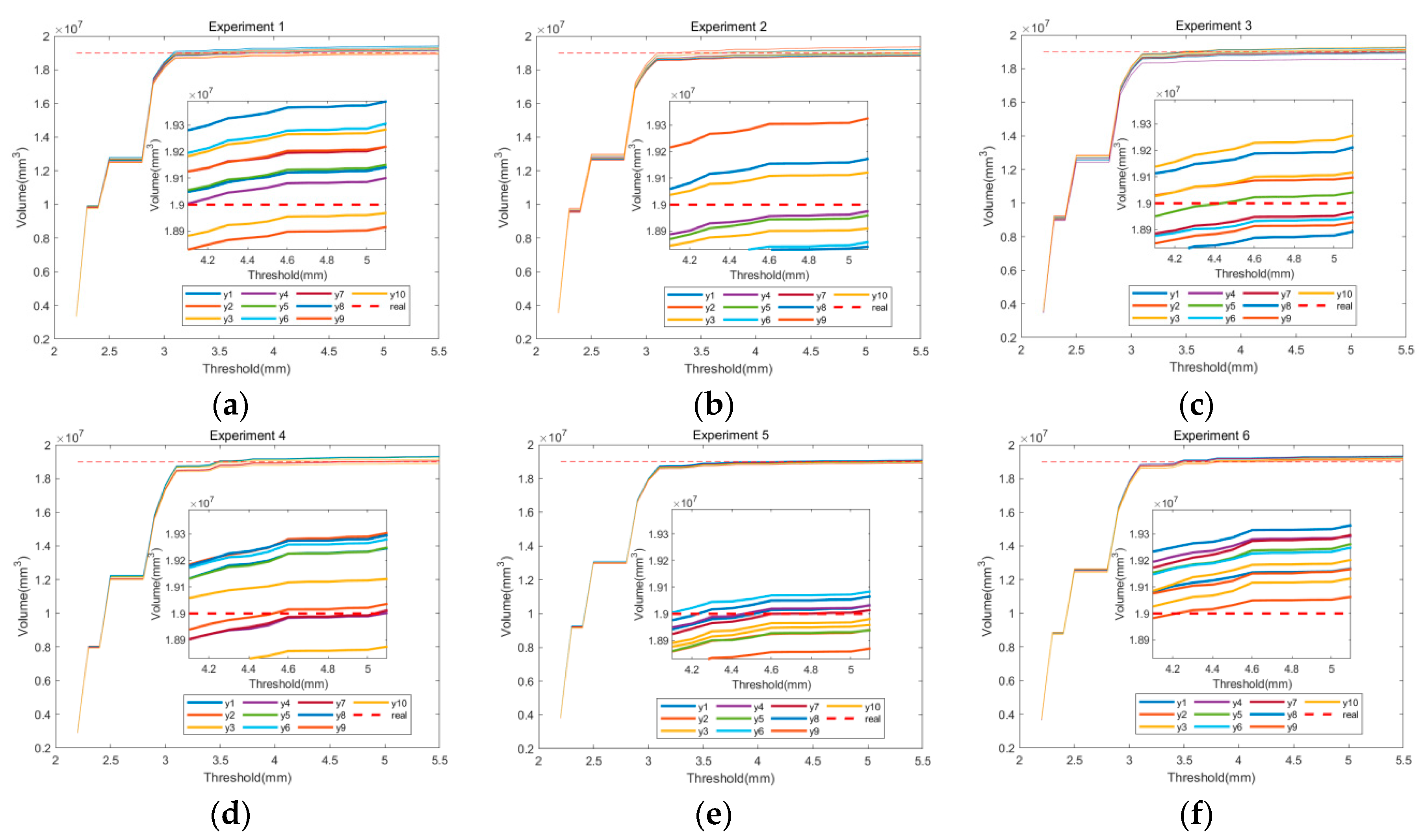
The study conducted six experiments using 31 different threshold ranges, ranging from 2.5 mm to 5.5 mm with a difference of 0.1 mm between each group. The experiments were performed on six different grain pile models, each representing a specific shape: flat, left-leaning, right-leaning, convex in the middle, concave in the middle, and grain piles that did not completely cover the container. Each experiment group consisted of ten measurements. The grain pile volume obtained through the binocular structured light system is illustrated in Figure 17. The figure displays the ten measurement results represented by dashes, while the solid line indicates the actual volume value of 0.019 m³.

Based on observations from Figure 17, it was noted that the measured volume of grain heaps with different shapes (flattened, left-tilted, right-tilted, convex, and concave) remained relatively stable when the threshold value exceeded 3.5 mm. No significant variations were observed beyond this threshold. This experimental design enabled the study to draw important conclusions about the impact of threshold range on grain heap volume measurement.

The volume measurements for different grain heap shapes were found to be relatively stable and tended to approach the true values, especially for threshold values exceeding 3.5 mm. This suggests that using these threshold values can lead to more reliable measurement results. These findings have important practical implications for selecting and optimizing grain heap volume measurement methods in grain storage and related fields. Additionally, this study offers a rational approach for selecting the threshold range and determining the number of experiments, which enhances the reliability of the research findings.

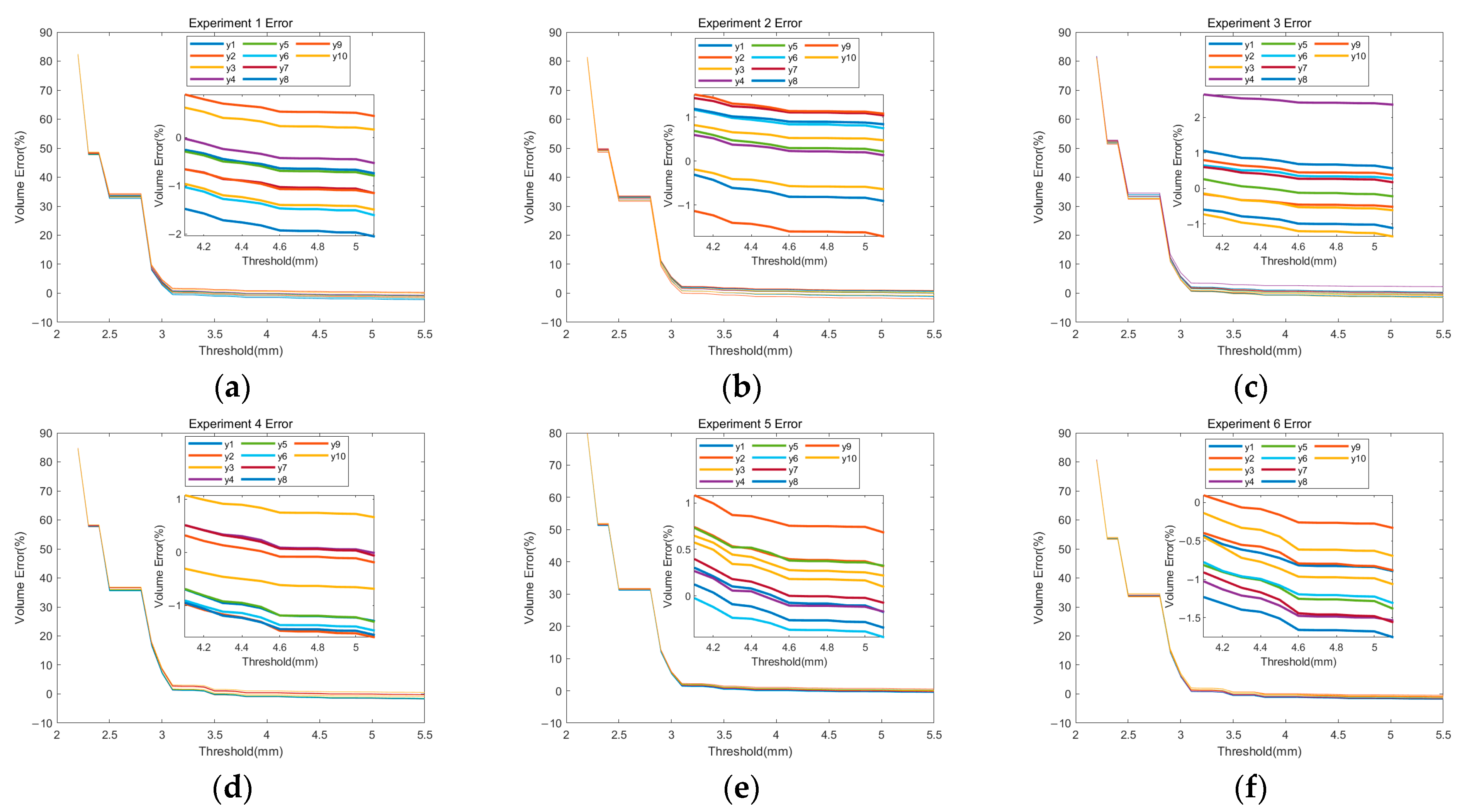
Experiments 1 to 6 in Figure 18 represent ten sets of measurement results for five different scenarios: grain pile flat, grain pile left inclination, grain pile right inclination, grain pile convex, grain pile concave, and the grain pile does not fully cover the container. These figures show the relative errors between the measured volume and the true volume. From the graphs, the following observations can be made: When the threshold is greater than 4 mm, the error is less than 1.5%; between the threshold values of 2.2 mm and 3 mm, the error gradually decreases; and when the threshold is greater than 4.6 mm, the error starts to increase again. This indicates the impact of the threshold on the volume measurement results. When the threshold is set too low, a significant number of holes are present in the formed triangular mesh, which results in considerable errors in volume measurement. As the threshold value increases, the number of divided triangles also increases, and the occurrence of holes gradually decreases. This reduction in holes leads to a decrease in errors in volume measurement. However, if the threshold is set too high, inconsistencies or incompleteness may arise in the triangles along the boundaries, resulting in an increase in volume and consequently an increase in measurement errors.

In practical applications, it is important to strike a balance and make adjustments when selecting a threshold. By choosing an appropriate threshold range, accurate volume measurements can be achieved while keeping errors within an acceptable range. The results shown in Figure 18 offer valuable insights for measuring grain pile volume and provide guidance for selecting the optimal threshold and optimizing volume measurements in practical scenarios. Taking into account both accuracy and computational efficiency, a threshold range greater than 4 mm can be chosen to obtain consistent and realistic volume measurement results.

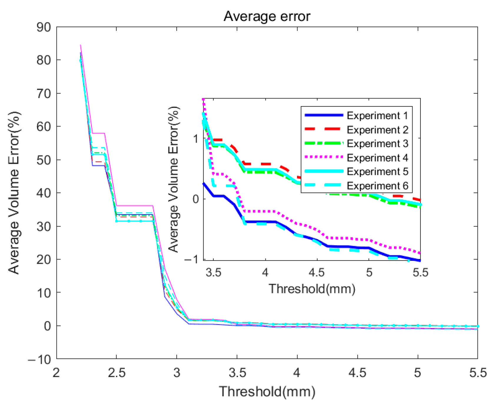
Figure 19 illustrates the relationship between the threshold and the mean error of the measurement volume. The experiments are labeled as Experiment 1 to Experiment 6, representing six distinct experiments with a flat grain pile, a grain pile with left inclination, a grain pile with right inclination, a convex grain pile, a concave grain pile, and a grain pile that does not fully cover the container. By analyzing the data in the graph, we can draw the following conclusions: when the precision (mean error) requirement is within 1%, choosing a threshold range between 3.5 mm and 5 mm can meet the requirement, and even within the range of 4 mm to 4.2 mm, the mean error can be within 0.5%. Since the shapes of grain piles in practical applications can be diverse, ensuring the applicability of the measurement system to different shaped grain piles is crucial.

We can observe that the method proposed in this study can achieve high-precision volume measurement results for the six different scenarios. This demonstrates that the method designed in this study has good applicability and stability for differently shaped grain piles.

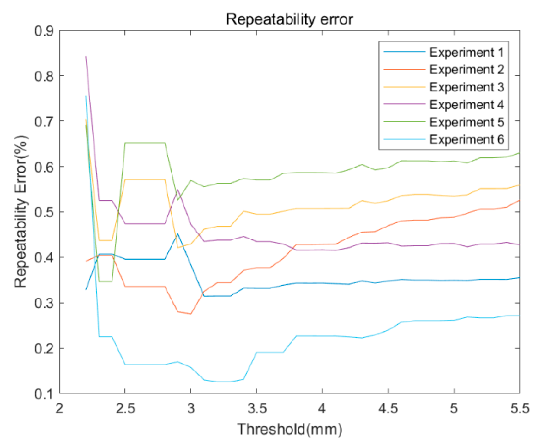
Figure 20 illustrates the relationship between the threshold and the repeatability error of the measurement volume (expressed as the relative standard deviation). The experiments are labeled as Experiment 1 to Experiment 6, representing six distinct experiments with a flat grain pile, a grain pile with left inclination, a grain pile with right inclination, a convex grain pile, a concave grain pile, and a grain pile that does not fully cover the container. The repeatability error shown in Figure 20 is an important indicator for evaluating the reliability of the measurement system. It is represented by calculating the experimental standard deviation to assess the repeatability of the measurement system and is expressed as the experimental standard deviation divided by the average measurement value to represent the repeatability error of the system. In the experiments, multiple volume measurements were conducted to verify the stability and precision of the system. From Figure 20, it can be observed that the repeatability error is consistently below 0.6% within the threshold range of 3 mm to 5 mm. This indicates that within this specific threshold range, the measurement system demonstrates excellent repeatability, high stability in volume measurements, and a relatively low repeatability error. The results show that the designed binocular structured light measurement system has good accuracy and reliability. A repeatability error below 0.6% indicates that the system can produce relatively consistent and stable volume measurement results in multiple measurements. The stability of grain pile volume measurements is crucial for accuracy and reliability, particularly when multiple measurements are needed in practical applications. The proposed binocular structured light measurement system for grain pile volume measurement is proven to be superior and effective. By taking repeatability error into account, the system’s performance can be thoroughly evaluated, providing valuable insights for future practical applications and system optimization. This experimental design and result analysis hold significant practical value for grain storage management and related research and practice.

To determine the optimal threshold range for our system, we conducted extensive experimental research. In the experiments, we used 31 different threshold ranges, ranging from 2.5 mm to 5.5 mm, with a difference of 0.1 mm between each group. We determined the best threshold range by comparing the measurement results under different threshold ranges and comparing them with the ground truth values. Ultimately, we selected a threshold range of 4 mm to 4.2 mm, which provided good stability and repeatability while maintaining measurement accuracy.

The experimental results from Figure 19 and Figure 20 show that the grain pile volume measurement error can be kept within 1.5%, the average error can be kept within 0.5%, and the repeatability error can be kept within 0.6%. The following is an analysis of several factors that may lead to errors.

(1)

Due to the precision of the camera, it introduces systematic errors in the measurements.

(2)

When obtaining the true volume of the grain pile through drainage methods, it may be influenced by human interventions, such as uneven drainage or inaccurate measurements.

(3)

When segmenting the point cloud for the grain pile, the complexity of point cloud data and noise may result in incomplete segmentation, leading to errors.

(4)

Factors such as the temperature and camera positioning in the experimental environment may have an impact on the measurement accuracy of the binocular camera.

(5)

The deformation of grain storage containers due to grain compression may introduce measurement errors.

7. Conclusions

This paper utilizes the binocular structured light approach to measure the volume of grain piles. The process begins with image processing and the implementation of the SGM algorithm for stereo matching. This helps compute and optimize the disparity map, which in turn provides depth map and point cloud information. Next, a refined Euclidean clustering segmentation method, along with pass-through filtering, is employed to segment the point cloud and extract the surface point cloud information of the grain pile. Once the segmented surface point cloud of the grain pile is obtained, an improved Delaunay triangulation method, along with projection and gap filling techniques, is used to measure the volume of the point cloud.

The experimental results demonstrate that, with appropriate accuracy requirements, the average error can be achieved within 0.5%. The error between each group of measurements is also within 1%. Additionally, the repeatability error is controlled within 0.6%. It is important to note that these experiments were conducted in a laboratory environment. In practical engineering applications, when dealing with large grain warehouses, the errors may be even smaller due to the influence of grain pile texture details or local shapes, resulting in more stable and accurate error performance. However, further research and practice are still necessary to validate and optimize the applicability and reliability of the proposed method in real-world grain storage applications.

The proposed binocular structured light measurement system in this paper has shown promising results in measuring the volume of grain piles. In a laboratory setting, it has demonstrated high precision and stability. However, for practical engineering scenarios involving large-scale grain warehouses, further practical verification and improvement are necessary to ensure accurate and reliable volume measurements in complex real-world environments. In the subsequent study, our aim is to further investigate the system’s performance and reliability in real engineering applications by conducting additional experiments and tests on actual grain silos. We will also examine how different grain types may affect the measurement accuracy. Furthermore, we intend to expand the measurement range by utilizing multiple devices to cater to the requirements of large grain piles.