Analysis of the Spatial and Temporal Evolution and Driving Factors of Landscape Ecological Risk in the Four Lakes Basin on the Jianghan Plain, China

Abstract

Due to the complex ecological effects of the interactions between natural environmental evolution and anthropogenic interference, a series of longstanding environmental problems have severely exacerbated the vulnerability of watershed ecosystems. Landscape ecological risk (LER) assessment is suitable for exploring the extent of threats and the likelihood of adverse impacts to watershed ecosystems from multiple sources of risk. However, the specific LER and the role of diverse factors on LER in the Four Lakes Basin remain unclear. Hence, it is necessary to identify the spatiotemporal evolutionary characteristics of LER and the drivers of their interactions. In this study, the variations and driving factors of LER in the Four Lakes Basin from 2000 to 2020 were evaluated. Landscape disturbance index was selected to establish the LER measurement method. Spatial autocorrelation and the standard deviation ellipse method were employed to analyze the spatiotemporal changes in LER. To overcome the uncertainties in accurately assessing the interactions, we attempted to use the geographic detector model to quantitatively analyze the driving factors. The following results are indicated: (1) In the period from 2000 to 2020, the LER had spatially uneven distribution characteristics of low in the north-central and high in the east and south. The level of LER has been increasing. (2) The LER has characteristics showing significant spatial clustering distribution. However, the spatial convergence has diminished with time. (3) The development inclination of LER was different in the two stages. The first stage (2000–2010) showed diffusion, while the second stage (2010–2020) was concentrated to the northwest. (4) The two-factor enhancement of interactions between land use index and human disturbance (q₂₀₀₀ = 0.885, q₂₀₁₀ = 0.888, q₂₀₂₀ = 0.713) was the dominant factor influencing LER. This study can provide a theoretical reference for ecological restoration and promotion of ecosystem service functions in the Four Lakes Basin.

1. Introduction

Landscape ecological risk (LER) refers to the possible adverse consequences from the interaction of landscape patterns and ecological processes under the influence of natural or anthropogenic factors [1]. As a vital sub-field of ecological risk assessment, LER assessment can efficiently optimize and integrate regional landscape patterns together with the sustainable development of environment and resources [2,3,4]. Analyzing the spatiotemporal evolution characteristics based on the evaluation of LER can determine the potential adverse effects from the existence of regional ecosystems under spatial and temporal changes. It provides support for environmental protection and ecosystem management [5,6]. Hence, studying the spatiotemporal dynamic evolution of LER and its socioecological effects is vital to better understand the relationship between ecosystems.

LER assessments can basically be divided into two categories based on risk source sinks and landscape patterns [7]. The early evaluation method benchmarks are dominated by the former, inheriting the basic principles of traditional ecological risk evaluation. However, it is suitable for the assessment objectives with specific regional ecological security risk coercion or clear stress factors on ecosystems [8,9,10]. The evaluation method based on landscape pattern analysis has eliminated the general process of traditional ecological risk assessment to a certain extent, from risk source identification to receptor analysis and finally exposure and hazard assessment [1]. The hot spot of research regarding the assessment system is the use of land use/cover change (LUCC) as a causative factor to describe the impact of manifold risk factors, such as human disturbance or natural change [11,12,13]. LUCC has been shown to be an applicative scope for exploring the spatial and temporal differentiation characteristics on ecosystems [14,15,16]. Within the framework of this study, the landscape pattern not only determines the form of resource and environmental distribution [17] but also quantifies the LUCC. Therefore, taking the landscape pattern as an entry point, a landscape index was constructed, integrating fragmentation, dominance, and separation of landscape structure to describe the LER [18]. LER assessment focuses more on the coupled correlation perspective of ecological processes and spatial patterns by constructing a sampling grid, which divides it into multiple risk areas to provide a more accurate spatial representation of risk [6]. Based on the assessment, substantial literature has appeared around the theme of different scale ranges, such as administrative divisions [19,20,21], watersheds [22,23,24,25], wetland [26], and coal mine area [4]. However, these studies focus on the time–space distribution characteristics and comparisons of LER, and lack exploring the impact of multiple driving mechanisms interacting on LER. Thus, it is necessary to evaluate the expression of risk in ecological functions and processes resulting from spatial and temporal patterns in combination with driving mechanisms for the construction of ecological environment security [27].

Against such a backdrop, exploring implications between natural and anthropogenic factors affecting regional LER has received increased attention in recent years [28,29,30]. Conventional methods for studying driving mechanisms, such as correlation analysis and classical regression models, can only describe the effect of factors on the trend in LER, and it is difficult to quantify the extent to which a factor affects the spatial divergence in LER [31]. Although geostatistics and geographically weighted regression can measure the spatial variability of ecogeographical phenomena, it is difficult to quantify the synergistic, antagonistic, or independent interactions between factors [32]. Compared with these methods, a geographic detector can quantify its driving factors with higher explanatory efficiency and detect interactions among two driving factors that are not possible with the classical geographic analysis [33]. As a statistical method, the geographic detector method measures spatial heterogeneity while also mining unique information incurred from spatial heterogeneity [34,35]. Based on this assumption, the following hypotheses were proposed:

H1: 

Spatial heterogeneity characterizes the distribution of LER.

H2: 

There are interactions among factors affecting the spatial heterogeneity in LER, and there are significant differences in the effects of the combined effects of the two factors on the distribution of LER.

As one of the important tributaries of the middle and lower reaches of the Yangtze River, the Four Lakes Basin is the main part of the Jianghan Plain in China. It connects the water cycle, biosphere, lithosphere, and other organic ecological systems with high ecological relevance across the region, providing a strong basis for regional biological reproduction and human activities [36,37]. However, the ecological environment of the Four Lakes Basin has been threatened by the seine farming and the development of urbanization in the region, together with the frequent occurrence of natural disasters. As an obviously ecologically fragile area, the Four Lakes Basin is chosen to be a study area.

Previous studies on the LER have focused on the characteristics of spatial patterns and trends in spatial and temporal variations. However, quantitative analysis of the interactions of the drivers affecting LER distribution is lacking and whether the combined effects of the driving factors have significant differences on LER. Therefore, this paper aims not only to reveal the rule of dynamic space–time patterns of change in the LER distribution, but also to quantify the degree and expression of interactions in the driving factors. In this study, we construct a LER evaluation model based on the results of LUCC. Spatial analysis models are used to explore the spatiotemporal evolution law of LER and the relationship between spatial associations in the study area. Identifying patterns in spatial and temporal variability and risk aggregation areas facilitate ecological management measures. With respect to the absence of analysis in comprehensive mechanisms, a geographic detector that combines multiple factors is applied to analyze the driving factors. Hence, this research has profound merit for understanding the mechanisms of LER change. Further, this research provides theoretical guidance for the prevention and control of LER in the Four Lakes Basin and serves as a valuable reference for other similar regions.

2. Study Area and Materials

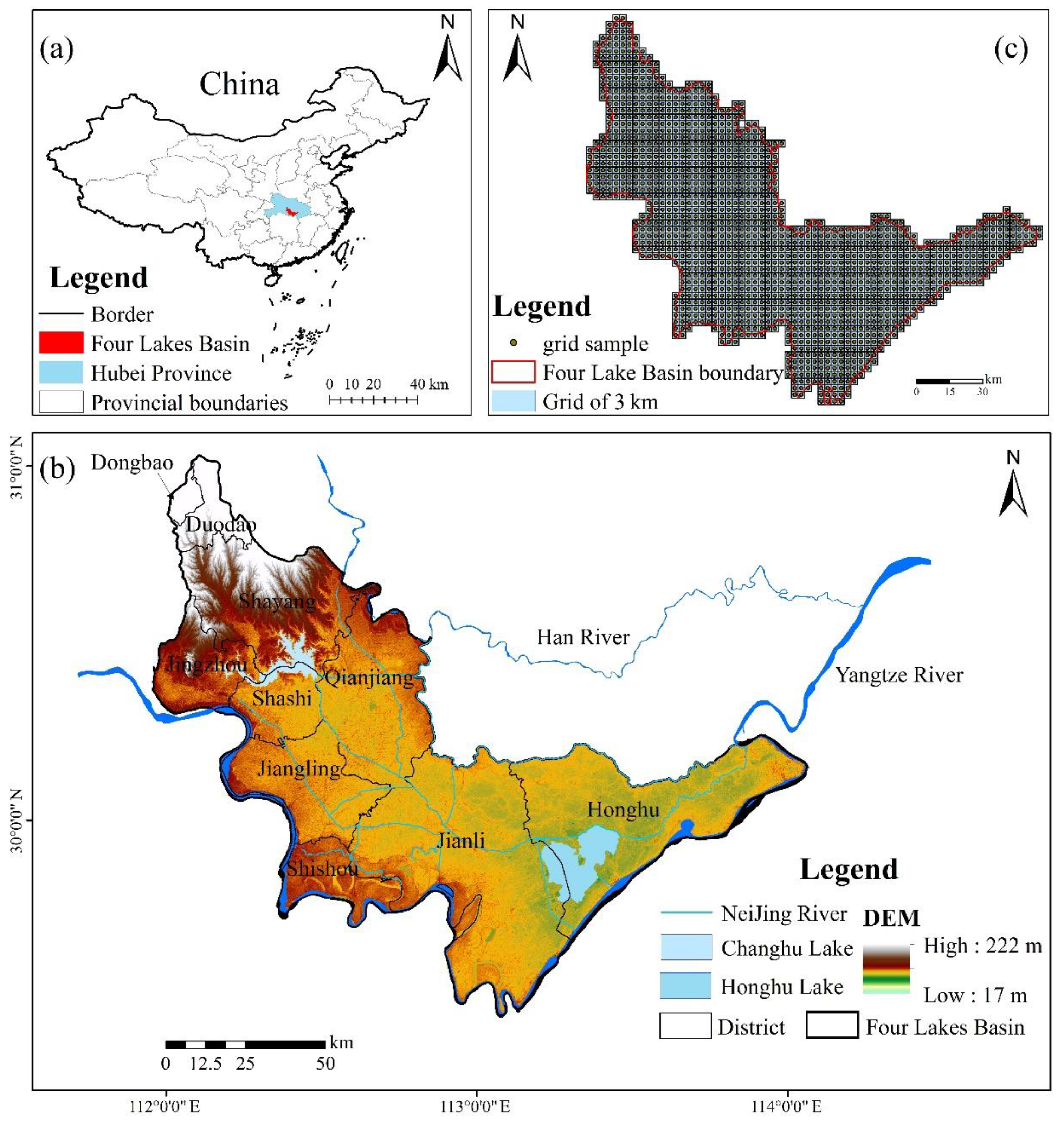
2.1. Study Area

The Four Lakes Basin on the Jianghan Plain (29°26′ N–31°02′ N, 111°58′ E–114°04′ E), is a depressional area between the Yangtze and Han rivers (Figure 1a,b), covering a total area of 11,547.5 km². There were four large lakes in the basin, namely Changhu Lake, Bailu Lake, San Lake, and Honghu Lake. It is known as the Four Lakes Basin due to the construction of canals connecting the four lakes. However, with the effect of reclamation and the evolution of the wetland environment, only two large lakes remain today, Changhu Lake and Honghu Lake. These two lakes play a pivotal role in human activities and the water supply and flooding of water conservancy projects. However, influenced by human activities, the two lakes also face long-standing environmental problems [38]. The total length of the trunk canal of the four lakes is 185 km, and it flows through Shashi District, Jingzhou District, Qianjiang City, Jiangling County, Jianli City, and Honghu City. It finally joins the Dongjing River through the Xintankou pumping station and converges into the Yangtze River.

The study area has a northern sub-tropical monsoon climate, with annual precipitation between 1100 and 1300 mm and annual average temperature between 15.7 and 16.6 °C. The area has sufficient light, with simultaneous rain and heat, flat topography, and fertile soil. Therefore, the Four Lakes Basin has become a prominent agricultural production base in Hubei Province. Additionally, it is a crucial part of the Yangtze River coastal economic belt. Under the impacts of climate change and human activities, the natural geomorphology and landscape of river and lake ecosystems in the region have been drastically disturbed. The watershed is experiencing long-term ecological and environmental problems [39].

2.2. Data Sources and Processing

The database used in this study is shown in

Table 1. Database sources.

Data	Time	Resolution	Source
Landsat 5/8 RS images	2000, 2010, and 2020	30 m	http://earthexplorer.usgs.gov/ (accessed on 11 May 2022)
DEM	-	30 m	https://www.gscloud.cn/ (accessed on 11 May 2022)
Rainfall and temperature	2000, 2010, and 2020	-	https://data.cma.cn/ (accessed on 11 May 2022)
MODIS-NDVI	2000, 2010, and 2020	250 m	https://modis.gsfc.nasa.gov/ (accessed on 12 May 2022)
Population density	2000, 2010, and 2020	1000 m	http://www.worldpop.org/ (accessed on 13 May 2022)

. The data processing procedure is shown below. (1) Geographic alignment and geometric correction were carried out for the series of Landsat remote sensing (RS) images. The error was controlled within 0.5 image elements, and image stitching and cropping were executed using ENVI5.3 software. The object-oriented random forest classification method was used to classify the pre-processed remote sensing images in eCognition 9.0 software. The images were visually corrected based on GPS field sampling points and Google Earth images. To facilitate the quantification of LER, the land use/land cover (LULC) types were classified into the following six categories: cultivated land, forest land, grass land, water body, construction land, and unused land. The overall accuracy of land cover classification was tested to be over 0.85, which meets the requirements for the study. The LULC types are shown in Figure 2. (2) Resampling to 30 m was used uniformly for data with different resolutions under ArcGIS 10.8.

3. Research Methods

The methodology used in this paper is divided into three parts. (1) Long time-series LER changes: By constructing LER evaluation model, we obtained the changes in LER during the period from 2000 to 2020. (2) Spatial analysis of LER: Two methods, spatial autocorrelation and standard deviation ellipse, were used to analyze the spatial clustering features and variation trends. (3) Analysis of driving factors of LER: A geographic detector was used to reveal the driving factors that influence and regulate LER. The technical route is shown in Figure 3.

3.1. Landscape Ecological Risk Assessment

3.1.1. Evaluation Cell Selection

To facilitate the analysis of the LER spatial distribution, a sampling grid was selected as the evaluation cell. The study area was divided according to the size of each risk cell by 2–5 times the area of the landscape patches [40]. The spatial grid sample (Figure 1c) was implemented for the study area according to the grid cell with a division area of 3 km × 3 km. There were a total of 1507 evaluation cells. The landscape ecological risk index (ERI) of the corresponding evaluation cell was extracted on the basis of the following ecological risk evaluation model. Ordinary kriging interpolation was performed on the ERI, and the ERI was classified into five levels, namely low, sub-low, medium, sub-high, and high risk using the natural breaks method.

3.1.2. Landscape Ecological Risk Evaluation Model

The objective of assessing the LER evaluation model was to assess the probability of adverse effects of landscape pattern changes on ecosystems at the landscape scale. Drawing on the existing research results of related scholars [11,41,42], the calculation formula was constructed as follows:

$$ERI={\displaystyle \sum _{i=1}^n\frac{A_{ki}}{A_k}{R}_i}$$

(1)

where A_k is the total area of the kth cell (km²); A_ki is the area of the ith LULC type in the kth cell (km²); and R_i represents the landscape disturbance index for the ith LULC type, which is expressed as follows:

$$R_i=F_i\times S_i$$

(2)

where F_i and S_i represent ecological vulnerability index and landscape loss index for the ith LULC type, respectively; the F_i values of the six LULC types are 1 for construction land, 2 for forest land, 3 for unused land, 4 for grass land, 5 for cultivated land, and 6 for water body [41]. S_i can be expressed as:

$$S_i=a{C}_i+b{N}_i+c{D}_i$$

(3)

where a, b, and c refer to the weights of C_i, N_i, and D_i, respectively, and the sum of a, b, and c is 1. In conjunction with previous research and the characteristics of the study region, in descending order of indicator importance are C_i, N_i, and D_i. Accordingly, a, b, and c are assigned values of 0.5, 0.3, and 0.2, respectively [12]. C_i, N_i, and D_i reflect landscape fragmentation index, landscape separation index, and landscape dominance index in a given LULC type, respectively, and they are calculated as follows:

$$C_i=\frac{n_i}{A_i}$$

(4)

$$N_i=\frac{A}{2A_i}\sqrt{\frac{n_i}{A}}$$

(5)

$$D_i=\frac{Q_i+M_i}{4}+\frac{L_i}{2}$$

(6)

where n_i is the patch number of ith LULC type; A_i is the area of ith LULC type (km²); A is the total area of the study area (km²); Q_i is the ratio of cells of ith LULC type to the total cells; M_i is the ratio of the number of patches of ith LULC type to the total number of all patches; and L_i is the ratio of the area of ith LULC type to the total study area.

3.2. Spatial Statistical Analysis

3.2.1. Global Spatial Autocorrelation and Local Spatial Autocorrelation

Global spatial autocorrelation reflects the degree of spatial correlation in landscape ecological risk from a macroscopic perspective. The global Moran’s I statistic judges the correlation dependence between data at a certain location and other locations within the distribution area [43]. The global Moran’s I can be expressed by the following equation:

$$Moran’s I=\frac{n}{S_0}\frac{{\displaystyle \sum _{i=1}^n{w}_{ij}{z}_i{z}_j}}{{\displaystyle \sum _{i=1}^n{z}_i^2}}$$

(7)

where n represents the number of spatial units studied; S₀ is the aggregation of all spatial weights; w_ij is the spatial weight between intervals i and j; and z_i and z_j are the deviation of the attributes of intervals i and j from their mean values, respectively. The positive and negative values and magnitude of the global Moran’s I measure the nature and degree of spatial aggregation in spatial autocorrelation, respectively.

To illustrate the clustering distribution patterns for ERI, the use of local spatial autocorrelation can better reflect the local spatial information, which is a good complement to global autocorrelation. The local Moran’s I (I) can be calculated as follows [44]:

$$I={\frac{n\left(x_i-\overline{x}\right){\displaystyle \sum _j^n{w}_{ij}\left(x_j-\overline{x}\right)}}{{\displaystyle \sum _i^n\left(x_i-\overline{x}\right)}}}_{{}_{}^{}}^{}{{}_{}^{}}_{{}_{}^{}}^{}{}_{}^{}\left(i\ne j\right)$$

(8)

where n is the number of spatial units; w_ij is the spatial weight, x_i and x_j are the ERI for the ith and jth spatial units, respectively; and $\overline{x}$ is the summary value for the ERI.

3.2.2. Standard Deviation Ellipse and Center of Distribution

Among many spatial statistical methods, the standard deviation ellipse (SDE) can accurately reveal centrality, spread, directionality, spatial morphology of geographic elements [45]. The spatial variation in ERI under different levels is finely delineated and quantitatively described by SDE. Its calculation formula is shown below:

$$\overline{X}=\frac{{\displaystyle \sum _{i=1}^n{w}_i{x}_i}}{{\displaystyle \sum _{i=1}^n{w}_i}}{,}_{}^{}\overline{Y}=\frac{{\displaystyle \sum _{i=1}^n{w}_i{y}_i}}{{\displaystyle \sum _{i=1}^n{w}_i}}$$

(9)

$$S=\pi {\sigma }_x{\sigma }_y$$

(10)

where ($\overline{X}$, $\overline{Y}$) are the coordinates for the weighted average center of gravity; n indicates the number of space cells; (x_i, y_i) denotes the latitude and longitude coordinates for each cell; w_i denotes the ERI corresponding to each cell; S denotes the area of the standard deviation ellipse; and σ_x and σ_y denote the standard deviation for the x and y axes of the ellipse, respectively.

3.3. Driving Factor Analysis

3.3.1. Extraction of Driving Factors

Considering the perspective of the environmental time domain and the characteristics of the research area, 10 driving factors were selected and categorized into anthropogenic and natural factors. For convenience of expression, x₁, x₂, x₃, x₄, x₅, x₆, x₇, x₈, x₉, and x₁₀ represent the maximum inter-annual normalized vegetation index (NDVI), farmland fragmentation, slope, land use intensity index (LUI), human disturbance (HD), annual precipitation, annual mean temperature, landscape diversity index, population density (PD), and administrative area, respectively. Based on the MODIS-NDVI of the listed years (Table 1), x₁ was analyzed using the maximum value synthesis method. x₂ as a landscape type was characterized using a composite score of integrated weighting factors [46]. Detailed indicators and the weights of indicators are presented in Tables S1 and S2. The specific formulas are shown as Equations (S1)–(S3). x₃ was evaluated based on DEM using surface terrain analysis tools. x₄ and x₅ were calculated by referring to the models constructed in the related studies [47,48], respectively. Specific methodological descriptions are reflected in the Supplementary Materials (Equations (S4) and (S5)). x₆ and x₇ were calculated from monthly rainfall and temperature for each year. Spatially interpolated maps of x₆ and x₇ were obtained for each weather station using ordinary kriging interpolation. x₈ was calculated using the modified Simpson diversity index under Fragstats 4.3 software. x₉ and x₁₀ were extracted by cropping the study area boundaries based on population density and the administrative boundaries of the study area, respectively.

3.3.2. Geographic Detector

The theoretical core of a geographic detector is to detect spatial differentiation and reveal its driving factors [35]. In this study, we explored three functions of the geographic detector, namely factor detection, interaction detection, and ecological detection to reveal the explanatory power, interaction effect, and significance effect of each driving factor on the spatial heterogeneity in the LER.

Factor analysis detects the spatial heterogeneity in Y, and evaluates the influence of factor X on the change in Y using the q-value. The q-value is a number between 0 and 1. A larger q-value represents stronger explanatory power of independent variable X on Y, and vice versa. The expressions are as follows [49]:

$$q=1-\frac{SSW}{SST}=1-\frac{{\displaystyle \sum _{h=1}^L{N}_h}{\sigma }_h^2}{N{\sigma }^2}$$

(11)

where SSW denotes the sum of variance within a stratum. SST denotes the total variance of the whole region; h = 1…L is the stratification of the dependent variable X or the independent variable Y; N_h and N represent the number of cells in stratum h and the whole region, respectively; σ_h² and σ² denote the variance of Y in stratum h and the whole region, respectively.

Interaction detection is used to identify the interactions between different risk factors and to assess whether the two factors together increase or decrease the explanatory power of dependent variable Y. The relationship between the two factors is divided into the following main cases, as presented in

Table 2. Interaction type of two factors.

Description	Interaction
q(X1 ∩ X2) < Min[q(X1), q(X2)]	Weakened, non-linear
Min[q(X1), q(X2)] < q(X1 ∩ X2) < Max[q(X1), q(X1)]	Weakened, single factor non-linear
q(X1 ∩ X2) > Max[q(X1), q(X2)]	Enhanced, double factors
q(X1 ∩ X2) = q(X1) + q(X2)	Independent
q(X1 ∩ X2) > q(X1) + q(X2)	Enhanced, non-linear

.

Ecological detection is used to compare whether the joint effect between two factors is significantly different on the spatial distribution of the dependent variable Y, as measured by the F-statistic:

$$F=\frac{N_{X1}\left(N_{x2}-1\right)SS{W}_{X1}}{N_{X2}\left(N_{x1}-1\right)SS{W}_{X2}}$$

(12)

where N_x1 and N_x2 denote the sample sizes of the two factors X1 and X2, respectively; and SSW_X1 and SSW_X2 denote the sum of the within-layer variance of the stratification formed by X1 and X2, respectively. The null hypothesis H₀ states that SSW_X1 = SSW_X2.

In this study, geographic detector analysis was performed in the R-Studio 4.2 environment using the “GD” package. The specific algorithm guidance is provided in the literature [50].

4. Results

4.1. Dynamic Changes in Landscape Ecological Risk

The spatial distribution of LER was calculated as explained in Section 3.1 (Figure 4a), and the results were depicted in a pie chart (Figure 4b). According to Figure 4a, the overall spatial distribution of LER level distribution varied significantly, showing the characteristics of being low in the north-central and high in the east and south. Combined with Figure 2, the distribution of landscape ecological risk was closely related to LULC. The distributions of the sub-high and high levels were generally consistent with the ponds and riverine areas. The lower areas were in the western and north-central areas, and were mainly hilly and urban and other construction areas. The landscape cover types were mostly woodland, built-up areas of towns, and other landscapes. The eastern and southern regions were mostly lakes, ponds, and dikes, together with river areas where the landscape type of which was mainly water mudflats. The landscapes were complex and variable, and landscape separation and fragmentation were extensive. Thus, LER was at a sub-high or high level. By analyzing the time series, the level changed dramatically, which is characterized by the continuous increase in the proportion of sub-high and high levels and the tightening in the proportion of low and sub-low levels. According to Figure 4b, the proportion of the high grade increased dramatically from only 2.28% in 2000 to 14.31% in 2020, increasing by 12.03%. From 2000 to 2010, the LER level was dominated by the sub-low level, accounting for 51.91% and 48.38%, respectively. However, in 2020, it changed to the sub-high level, accounting for 44.18%. The overall proportion of the sub-low level decreased by 31.86% from 2000 to 2020. This change indicates that the LER had increased significantly between 2000 and 2020. Especially over nearly past 10 years, the proportion of high and sub-high level had increased dramatically, indicating that the landscape ecosystem was under greater threat.

4.2. Spatial Analysis of Landscape Ecological Risk

4.2.1. Spatial Autocorrelation Analysis

By analyzing the global spatial autocorrelation, global Moran’s I for the spatial distribution of ERI in 2000, 2010, and 2020 were 0.542, 0.528, and 0.505, respectively (Figure 5a). It is clear from variation trends that the ERI was significantly positively correlated. The values were clustered and influenced each other spatially. However, global Moran’s I tended to decrease over time, inferring that the degree of spatial autocorrelation weakened and spatial convergence gradually decreased. This finding is also related to the imbalance in landscape pattern distribution caused by the LUCC.

To further explore the correlation and aggregation degree of LER in local space, the spatial distribution in the clustering map for local Moran’s I (LISA) from 2000 to 2020 was plotted (Figure 5b). It shows that the ERI is mainly in distributions of H-H and L-L. The distribution area has been relatively stable over time, with less anticorrelated aggregation patterns such as L-H and H-L. This indicates that the LER shows significant spatial distribution differences. Figure 5b shows that during the period from 2000 to 2010, the high value areas are mainly clustered in the eastern and southern regions. The low value areas are mainly clustered in the western and northern regions. With the passage of time, the local spatial autocorrelation results in 2020 showed that there was mainly an H-H partition, which is consistent with the distribution area in the previous period. The distribution range is spread, and the low-low partition has a very small distribution area, indicating that the LER is basically concentrated in the local high-value distribution. Indirectly, it can be inferred that the impact on the local space during 2010–2020 intensified. The threat to the local ecological environment has been further enhanced.

4.2.2. Spatial Pattern Change Analysis

By drawing the SDE distribution and the center of the variations in different LER levels in the study area from 2000 to 2020 (Figure 6), the relative spread of risk and the trajectory and spatial displacement of the center of each level can be described. In addition, the results further determine the direction of the alteration in LER and whether the development shows a concentrated or diffuse developmental trend. The results revealed that both high and low grades moved significantly to the west and northwest during 2000–2020, where the spatial displacement of the center of low and sub-low grades moved from the northern part of Honghu city to Qianjiang city, and the center of sub-high and high grades shifted from Jianli city to Qianjiang city. The medium-grade center is concentrated in southern Qianjiang city.

Through spatial statistical analysis, according to the results in

Table 3. Characteristic ellipse parameters for the landscape ecological risk levels.

ERI Level	Year	Longitude	Latitude	Long Half-Axle/km	Short Half-Axle/km	Elliptic Area/km2
Sub-low and low	2000	113.35	30.09	81.24	35.85	9147.24
	2010	113.24	30.08	88.41	37.73	10,478.09
	2020	112.62	30.28	73.55	32.93	7607.22
Medium	2000	112.77	30.18	78.37	39.63	9756.64
	2010	112.69	30.14	68.03	42.56	9095.53
	2020	112.68	30.16	66.34	30.61	6377.59
Sub-high and high	2000	113.07	29.98	79.5	42.95	10,726.71
	2010	113.1	30.07	86.77	47.23	12,875.41
	2020	112.58	30.39	59.01	28.23	5232.24

, the development trend in the low and sub-low levels was consistent with that for the high and sub-high levels. The value change in the SDE area gradually increased during the period from 2000 to 2010, indicating that the development tended to spread in the early stage. However, the SDE area decreased during 2010–2020. From 2010 to 2020, the LER was concentrated in the northwest direction.

4.3. Importance Analysis of Driving Factors

The factor detector can detect not only the spatial heterogeneity in LER, but also the extent to which the driving factors explain the spatial heterogeneity. By means of single factor detection, the explanatory power map of the driving factors was calculated based on q-values. As shown in Figure 7, LUI (x₄) ranked first in terms of its contribution to the spatial differentiation of LER, with q-values of 0.785, 0.781, and 0.646. This result indicates that LUI was the predominant factor controlling the variation in the period from 2000 to 2020. It was followed by the HD (x₅). Additionally, the q-value for anthropogenic disturbance revealed an overall increasing tendency, from 0.576 in 2000 to 0.613 in 2010 and slightly decreasing to 0.577 in 2020. This implies that the intensity of anthropogenic disturbance in the landscape is gradually becoming one of the leading factors controlling the spatial variability of LER. The natural elements were under the implication of long-term environmental factors, and the q-value generally fluctuated between 0.1 and 0.2 during 2000–2010, with a more stable influence. The q-value increased for the annual precipitation (x₆) and reached 0.12 in 2020 under the effect of extreme precipitation events in the middle and lower reaches of the Yangtze River, increasing to 0.234. These results also indicate the impact of extreme climate on LER. However, the overall driving factors affecting the greater LER were anthropogenic factors such as LUI (x₄) and HD (x₅).

4.4. Ecological Analysis of Driving Factors

Ecological detection in the geographic detector allows us to determine whether there are significant differences in the effects of the above variables on the spatial distribution of LER. This method mainly compared the differences between factors. The detection results were tested using a t-test with a significance level of 0.05. As shown in Figure 8, most of the factors differed significantly from each other. There were only a small number of factors with too large or too small differences due to the q-value data. These were between farmland fragmentation (x₂) and NDVI (x₁), and between annual precipitation (x₆) and annual mean temperature (x₇). Hence, there was no significant difference in the interaction for these factors in the statistical analysis.

5. Discussion

5.1. Spatial and Temporal Variation in Landscape Ecological Risk

The landscape patterns of LUCC are strongly associated with ecological risk [51,52]. LER was characterized by obvious spatial heterogeneity. The spatial distribution of LER in the study area was low in the northwest and higher in the south and southeast. The regions with lower LER ranks were primarily influenced by forest land and grass land. Causes of higher LER rank were mainly affected by construction land, with more enhanced development and urbanization levels. This result was consistent with the findings from watersheds in China and foreign countries with different ecological conditions, such as the Bosten Lake Basin [53], Bailong River Basin [54], Red River Basin [55], and typical cross-border Koshi River Basin [42]. As a result of human reclamation of lakes and climate change, the trend in shrinking water bodies has increased [56] and the number of patches has decreased. Additionally, the water bodies themselves have a high degree of landscape vulnerability [41], leading to an increase in the degree of landscape disturbance and vulnerability. Similar to the Lake Shengjin wetland [57], Three Gorges Reservoir Region [58], Manas River Basin [59], and Padam River Basin [60] in Bangladesh, high and sub-high LER levels were mainly located near water bodies.

The changes in the LER levels were characterized by a clear phase change. The ERI values have gone through two distinct periods of change over time. As shown in Figure 9, the LER shifted mainly from low to medium level during 2000–2010. From 2010 to 2020, industrial transformation and upgrading were promoted, strategy for “Industrialization of City” was implemented, and modern service industry was developed vigorously. Highway and railroad networks have been built to support industrial manufacturing and modern service. These artificial corridors of disturbance affected the connectivity of the regional ecosystem. Due to the obstruction of material and energy exchange between ecosystems, the spatial–temporal differentiation and dispersion of ecological landscape patches increase [16]. Hence, the level shifted mainly from medium to sub-high level as well as from sub-low to sub-high level, indicating there was a trend toward increasing risk in the landscape of the Four Lakes Basin.

The spatial and temporal evolutions in both LER and ecological vulnerability in the watershed are strongly coupled with landscape pattern indices characterizing landscape diversity, fragility, and separation [61]. This study showed that the variations in LER were consistent with the trends in landscape fragmentation. Based on the characteristic of ERI as determined by changes in landscape type assemblages and their vulnerability [62], the landscape pattern indices based on the number, distribution aggregation, connectivity, and diversity were selected. The specific indicators included the number of patches (NP), patch density (PD), agglomeration index (COHESION), dispersion index (SPLIT), and Shannon diversity index (SHDI). The indicators of landscape pattern changes in the watershed at different times were counted (

Table 4. Changes in the landscape level pattern index in the Four Lakes Basin.

	Year	2000	2010	2020
Index
NP		11,762	13,661	17,676
PD		0.9762	1.1338	1.467
COHESION		99.7077	99.6875	99.3485
SPLIT		23.0178	23.2429	60.8445
SHDI		1.6387	1.6866	1.7736

). Against the backdrop of measures to promote urban–rural integration and expand the capacity of county-level cities in the western part of the basin, natural and semi-natural landscapes have been encroached upon. The invasion and fragmentation of human landscapes has led to a decline in the quality of the regional natural ecosystems [63] and exacerbated landscape ecological vulnerability. Due to the high-intensity urban sprawl, it has significantly changed landscape patterns in the study area, shattering other landscape types and bringing challenges to watershed ecosystems. Ramping up the degree of landscape vulnerability has become the main driving factor in the higher LER [64]. The ERI is trending downward in the Padam River Basin due to an overall decrease in NP and an increase in landscape integration [60]. Different from this watershed, the indicators NP, PD, and SPLIT, which characterize landscape fragmentation, increased during the last 20 years. The higher the landscape fragmentation is, the weaker the connectivity. The increased spatial and temporal differentiation and dispersion of landscape patches resulted in higher regional landscape fragility. The increase in SHDI, which represents landscape diversity, changes the landscape dominance and further affects ERI. The development trend in LER exhibited a northwest clustering pattern and a further enhancement, indicating the stage change and spatiotemporal distribution characteristics of the results.

Based on the rule of LER variation applied to ecological protection and restoration work in the watershed, different risk response measures should be adopted according to different risk level areas. For LER clustering areas such as the eastern and southern regions, land use should be rationally planned to reduce the fragmentation of ecological land. It is vital to implement the “Yangtze River Protection” policy and continue to strengthen comprehensive improvements for the Yangtze River shoreline. Cultivated land and transition area between water body and construction land are in areas of sub-high and medium level. Thus, fragmentation of farmland patches can be reduced through land preparation projects. Rewetting projects should be conducted to minimize landscape vulnerability in the watershed. Regarding low and sub-low LER regions, return of farmland to forest and soil and water conservation should be carried out actively. A comprehensive ecological compensation mechanism should be established to prevent a northwest clustering development trend and ensure sustainable development of economic, social, and ecological assets [65,66].

5.2. Sensitive Analysis of Input Data in the Geographic Detector Model

In the geographic detector model, geographical continuous variables need to be discretized [35]. Due to the uncertainties associated with the input data and model parameters, the spatial data discretization and scale effects are vital issues. However, they are generally determined by experience and lack accurate quantitative assessment. Due to the spatially stratified heterogeneity perspective, higher q-values indicate greater importance of the variables. Against this backdrop, we used q-value to identify the best parameter combinations by optidisc function in the “GD” package. This function can automatically calculate the optimal method and classification by an algorithmic procedure. The optimal discretization parameter is an integration of discretization and break number for continuous variables [50]. The discretization methods used mainly included equal interval (equal), quantile (quantile), natural breaks (natural), standard deviation (sd), and geometry interval (geometric). To better compare with LER levels, we set the breakpoints of the variables to 4 and 5. Taking 2020 as an example, the processes of parameter optimization for spatial data discretization are shown in Figure 10. Tests illustrate that optimal discretization parameters are varied for different explanatory variables. For LUI (x₄), when the q-value is maximum, the optimal parameter is the equal interval method with five breakpoints. Optimization of the discretization process aims to obtain a more accurate spatial analysis and subsequent study of the driving mechanisms.

5.3. Landscape Ecological Risk under Multiple Driving Mechanisms

The LER dynamics were affected by multiple factors, such as topography [32], meteorological condition [30], and anthropogenic interference [6]. For Zoige Plateau [67] and transboundary Gandaki River Basin [68], typical of alpine wetland ecosystems worldwide, the dominant factors influencing the divergence of LER are elevation and climate. Different from these plateau watersheds, the leading factors affecting LER of Four Lakes Basin located on the Jianghan Plain are anthropogenic factors. The impact of other natural factors is more balanced (Figure 7).

Driving factors not only affect the ecological environment, but also influence it synergistically, mainly including non-linear and two-factor enhancement [69]. Interaction detection is spatially overlaid in a geographic detector to quantitatively identify the effect of the driving factors on the landscape ecological risk after interaction. In this study, we used interaction analysis to seek the explanatory power for the interaction between factors on the distribution of spatial heterogeneity in LER. The single-factor q-value map (Figure 7) and the multifactor interaction influence bubble map (Figure 11) show that the spatial and temporal heterogeneity in the landscape ecological risk pattern was characterized by the combined effect of natural and socioeconomic factors. Consistent with previous studies [13,66,70], the analysis of driving factors showed that the spatially heterogeneous distribution in LER that affects the study region remains a pattern developed and guided by the role of anthropogenic activities. Similar to the Shule River Basin [71], the interaction of natural and anthropogenic factors was significant in influencing the heterogeneity in landscape ecological risk. Compared with the role of natural factors alone, the synergistic effect of natural factors and anthropogenic factors had stronger explanatory power. The interaction between anthropogenic factors was significantly stronger than the interaction between natural factors. In terms of the effects of the interactions, the interactions between the factors were all non-linearly and double-factor enhanced. It can be inferred that the double-factor effects are far more influential than the single-factor effects. The explanatory strength of the interactions between LUI (x₄) and HD (x₅) was the highest in all three periods (q₂₀₀₀ = 0.885, q₂₀₁₀ = 0.888, q₂₀₂₀ = 0.713), showing a multifactor-enhanced interaction scenario.

Changes in landscape patterns result from a combination of various natural and anthropogenic disturbance factors, which influence ecological processes and edge effects, and directly affect changes in LER [72]. As an indispensable part of the Yangtze River economic belt, the Four Lakes Basin has been transformed in the last 20 years by the urbanization process, with rapid economic development and a surge in anthropogenic disturbances due to the intensification of human activities. During 2010–2020, the basin continued to promote industrial growth and upgrading—the “Thousand Enterprises and Hundred Billion Technical Reform Project” was implemented. Further, the differentiated development of county-level cities and industries aimed to create multiple urban core areas and form municipal sub-centers. These processes have led to the disruption of the material and energy flows in the ecosystem covering the land surface. The distribution pattern and functions of the environment have changed, which has resulted in a series of ecological problems, such as soil erosion, environmental pollution, habitat degradation, biodiversity reduction, and ecosystem imbalance, thus increasing the degree of ecological risk [73,74,75,76,77,78]. LUI and HD make it the dominant factor influencing the spatial heterogeneity in LER in the Four Lakes Basin. However, the decreasing explanatory power concerning the effect of LUI (x₄) and HD (x₅) interaction during the three periods indirectly indicates that there is an increasing synergistic effect of the other factors.

Affected by the complexity and evolving characteristics in a combination of long-term human activities and natural disturbances, urbanization sprawl should be controlled. Ecological buffer zones should be designed around important wetlands and key agricultural areas.

5.4. Limitations of Study and Future Work

The LER assessments have an advantage of quantitatively describing landscape structures and reflecting the risk evolution from the landscape prospective [79]. However, there are still some unavoidable uncertainties and limitations. First, the LER assessments are characterized by typical scale dependence. The selection of scale often depends on the researcher’s knowledge or the grain and extent of scale. Different grain and extent of spatial scale can directly cause bias in ERI [66,80]. Given the uncertainties concerning the scale, we will optimize the evaluation and selection cell of ERI. Eventually, there are several socioeconomic factors affecting LER [28], such as population growth, land use policies, economic activities, and urbanization rates. In subsequent research, we will consider these factors in our analysis to gain a greater awareness of the driving mechanisms.

6. Conclusions

In this study, we constructed the ERI based on the landscape index of LULC type. The study comprehensively analyzed the spatial and temporal evolutionary characteristics of LER by means of spatial analysis and statistics. This study quantitatively detected the evolutionary mechanism in LER by using a geographic detector model. The following conclusions were obtained.

(1)

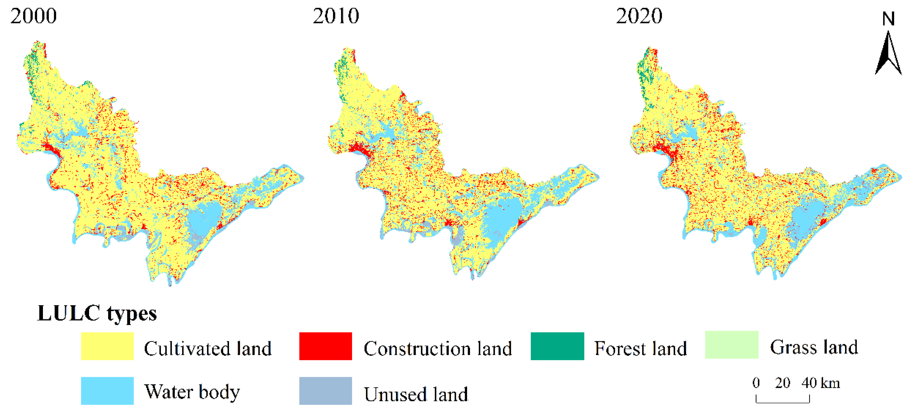
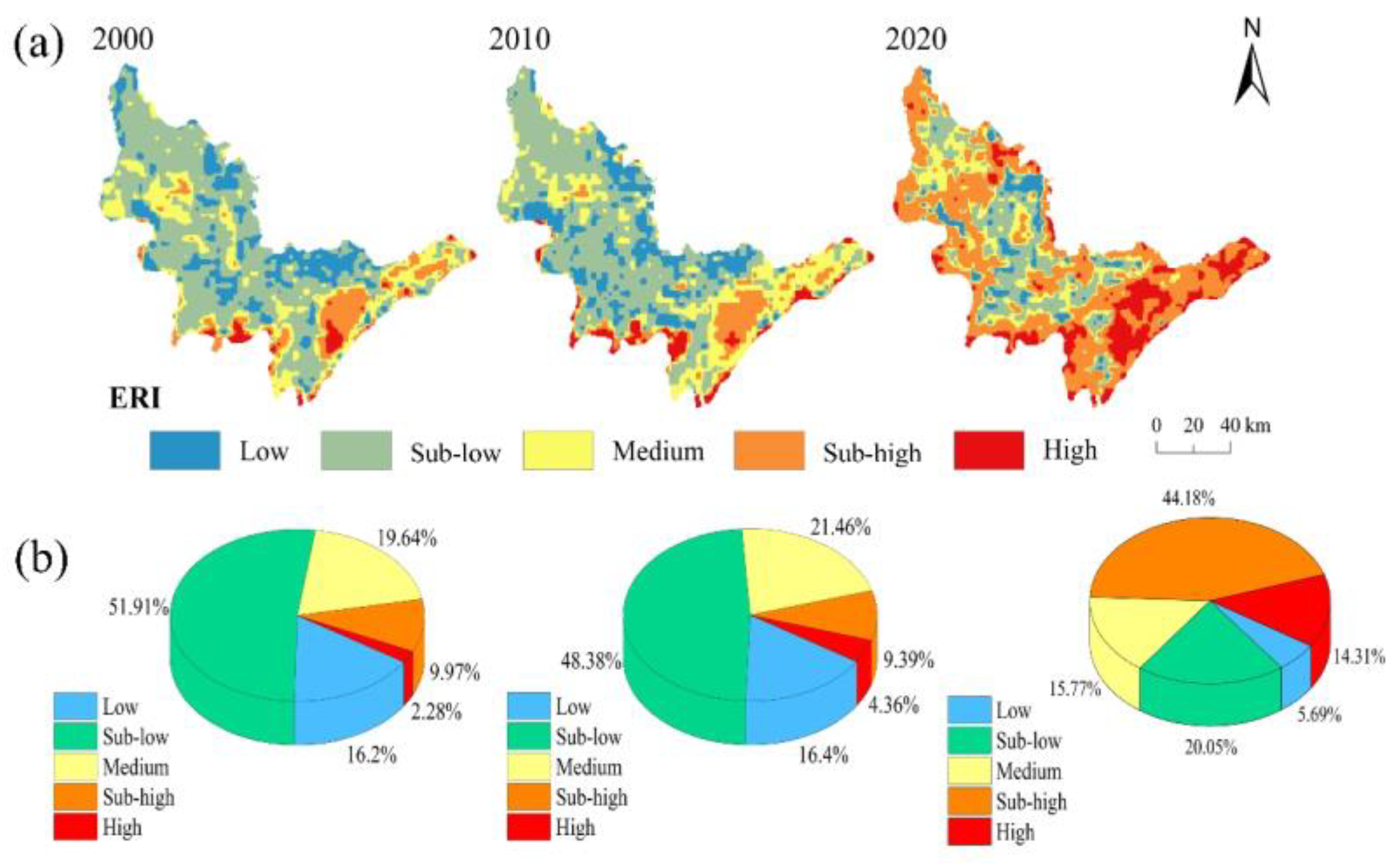
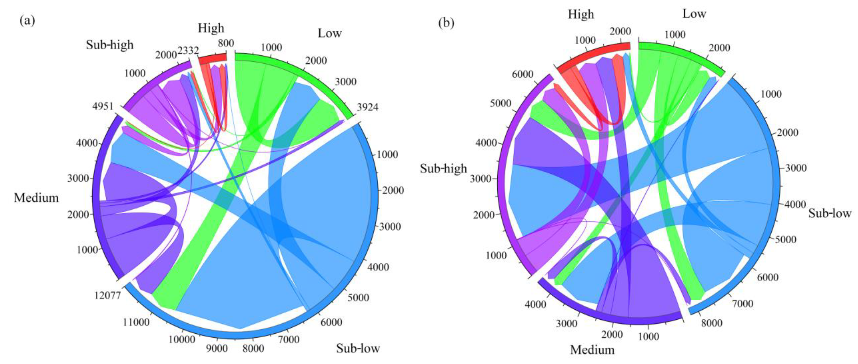
From 2000 to 2020, the level of LER in the Four Lakes Basin has shown strong and complex changes. In terms of the spatial distribution characteristics, the results mainly reflect high values in the east and low values in the north. During this time, the percentage of sub-low level decreased by 31.86% and the percentage of high level increased by 12.03%. The variations in the LER with time series showed a shift from low and sub-low to sub-high and high levels.

(2)

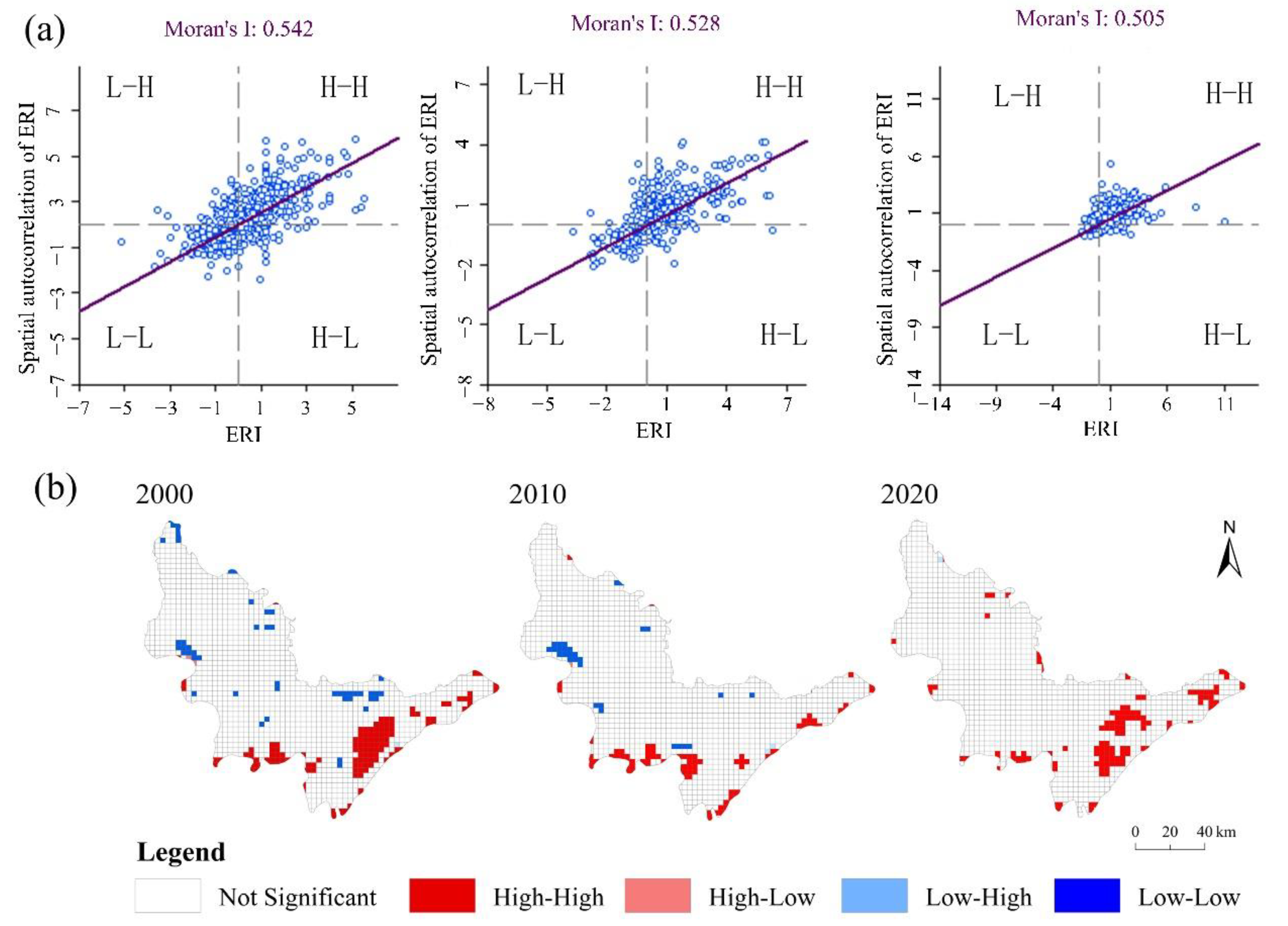
The global Moran’s I of LER declined from 0.542 to 0.505, indicating a clustered distribution in space with a spatial convergence and a weakening of global agglomeration over time. However, with the influence of human activities, the LER was mainly distributed in the local space with H-H clustering during 2010–2020.

(3)

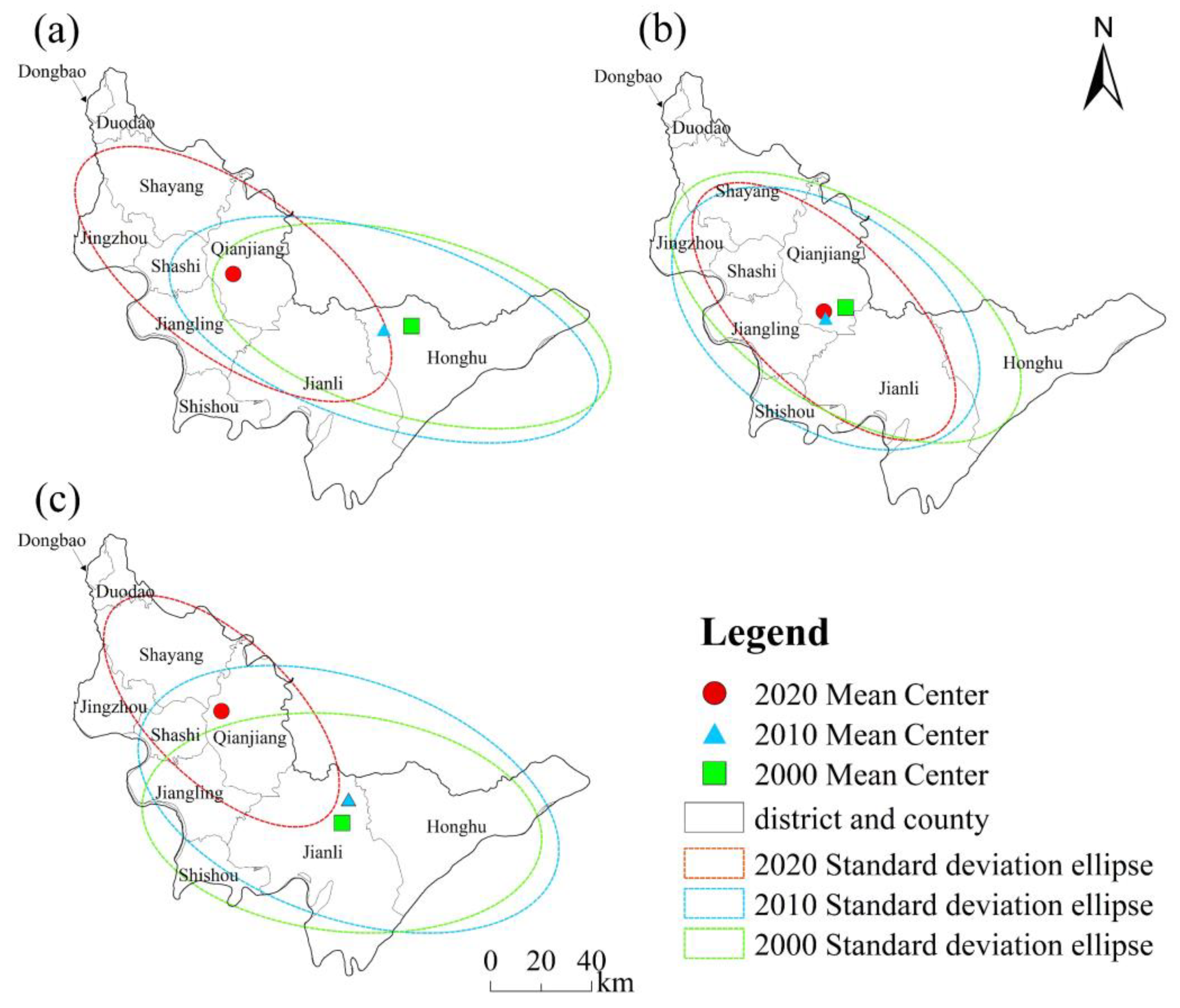
The center of the LER in the Four Lakes Basin shifted to the northwest. The center of sub-high and high level transferred from Jianli City to Qianjiang City. The changes in the parameters for the elliptical standard deviation of the LER showed diverse development trends in the two periods. The first period (2000–2010) manifested a diffusion trend, and the second period (2010–2020) manifested a concentrated development trend to the northwest.

(4)

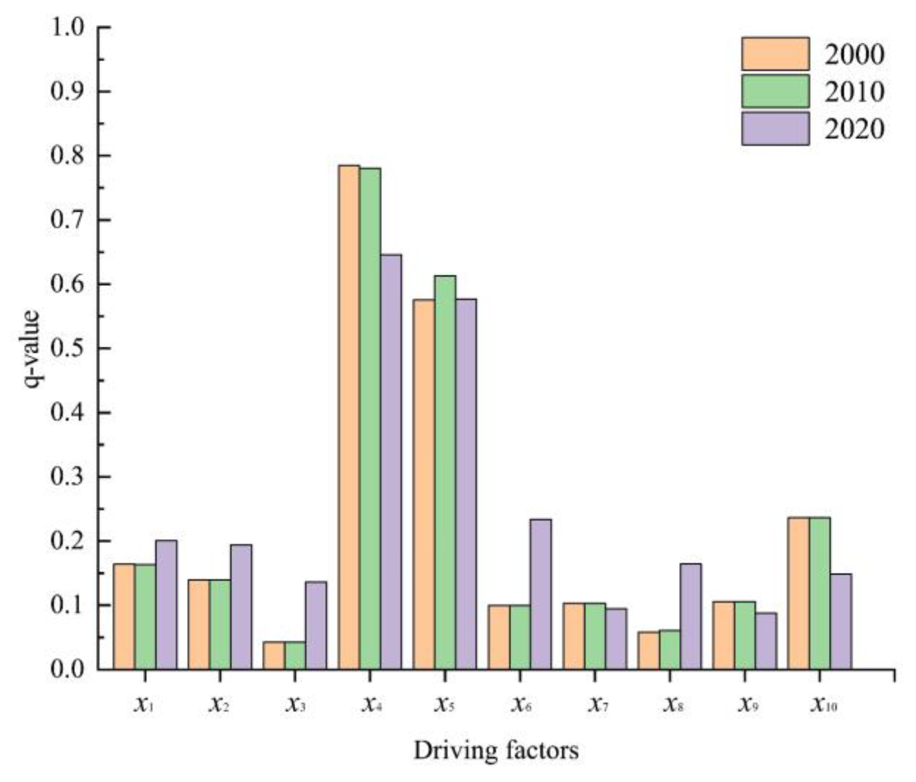
For an individual driving factor, LUI (q₂₀₀₀ = 0.785, q₂₀₁₀ = 0.781, q₂₀₂₀ = 0.646) plays a dominant role for the distribution of LER. The spatially heterogeneous distribution in LER affecting the Four Lakes Basin was caused by the interaction of double-factor enhancement and non-linear enhancement. Human disturbance and other natural factors had significantly different impacts on the spatial differentiation of LER in the Four Lakes Basin. The interactions between LUI and HD (q₂₀₀₀ = 0.885, q₂₀₁₀ = 0.888, q₂₀₂₀ = 0.713) were the leading driving factors of LER affecting the basin.

References

1. Peng, J.; Dang, W.X.; Liu, Y.X.; Zong, M.L.; Hu, X.X. Review on landscape ecological risk assessment. Acta Geogr. Sin. 2015, 70, 664–677. [Google Scholar]
2. Lei, K.; Pan, H.Y.; Lin, C.Y. A landscape approach towards ecological restoration and sustainable development of mining areas. Ecol. Eng. 2016, 90, 320–325. [Google Scholar] [CrossRef]
3. Piet, G.J.; Knights, A.M.; Jongbloed, R.H.; Tamis, J.E.; de Vries, P.; Robinson, L.A. Ecological risk assessments to guide decision-making: Methodology matters. Environ. Sci. Policy 2017, 68, 1–9. [Google Scholar] [CrossRef]
4. Xu, W.X.; Wang, J.M.; Zhang, M.; Li, S.J. Construction of landscape ecological network based on landscape ecological risk assessment in a large-scale opencast coal mine area. J. Clean. Prod. 2021, 286, 125523. [Google Scholar] [CrossRef]
5. Levine, S.L.; Giddings, J.; Valenti, T.; Cobb, G.P.; Carley, D.S.; McConnell, L.L. Overcoming Challenges of Incorporating Higher Tier Data in Ecological Risk Assessments and Risk Management of Pesticides in the United States: Findings and Recommendations from the 2017 Workshop on Regulation and Innovation in Agriculture. Integr. Environ. Assess. Manag. 2019, 15, 714–725. [Google Scholar] [CrossRef] [PubMed]
6. Lin, Y.Y.; Hu, X.S.; Zheng, X.X.; Hou, X.Y.; Zhang, Z.X.; Zhou, X.N.; Qiu, R.Z.; Lin, J.G. Spatial variations in the relationships between road network and landscape ecological risks in the highest forest coverage region of China. Ecol. Ind. 2019, 96, 392–403. [Google Scholar] [CrossRef]
7. Wu, J.G. Landscape sustainability science: Ecosystem services and human well-being in changing landscapes. Landsc. Ecol. 2013, 28, 999–1023. [Google Scholar] [CrossRef]
8. Loibl, W.; Smidt, S. Ozone exposure Areas of potential ozone risk for selected tree species in Austria. Environ. Sci. Pollut. Res. 1996, 3, 213–217. [Google Scholar] [CrossRef]
9. Landis, G.W. Twenty Years Before and Hence; Ecological Risk Assessment at Multiple Scales with Multiple Stressors and Multiple Endpoints. Hum. Ecol. Risk Assess. Int. J. 2003, 9, 1317–1326. [Google Scholar] [CrossRef]
10. Ran, P.L.; Hu, S.G.; Frazier, A.E.; Qu, S.J.; Yu, D.; Tong, L.Y. Exploring changes in landscape ecological risk in the Yangtze River Economic Belt from a spatiotemporal perspective. Ecol. Ind. 2022, 137, 108744. [Google Scholar] [CrossRef]
11. Zhang, F.; Ayinuer, Y.S.J.; Wang, D.F. Ecological risk assessment due to land use/cover changes (LUCC) in Jinghe County, Xinjiang, China from 1990 to 2014 based on landscape patterns and spatial statistics. Environ. Earth Sci. 2018, 77, 491. [Google Scholar] [CrossRef]
12. Jin, X.; Jin, Y.X.; Mao, X.F. Ecological risk assessment of cities on the Tibetan Plateau based on land use/land cover changes–Case study of Delingha City. Ecol. Ind. 2019, 101, 185–191. [Google Scholar] [CrossRef]
13. Chen, J.; Dong, B.; Li, H.R.; Zhang, S.S.; Peng, L.; Fang, L.; Zhang, C.B.; Li, S. Study on landscape ecological risk assessment of Hooded Crane breeding and overwintering habitat. Environ. Res. 2020, 187, 109649. [Google Scholar] [CrossRef] [PubMed]
14. Newbold, T.; Hudson, L.N.; Arnell, A.P.; Contu, S.; Palma, A.D.; Ferrier, S.; Hill, S.L.L.; Hoskins, A.J.; Lysenko, I.; Phillips, H.R.P.; et al. Has land use pushed terrestrial biodiversity beyond the planetary boundary? A global assessment. Science 2016, 353, 288–291. [Google Scholar] [CrossRef] [PubMed]
15. Bhattachan, A.; Emanuel, R.E.; Ardon, M.; Bernhardt, E.S.; Anderson, S.M.; Stillwagon, M.G.; Ury, E.A.; Bendor, T.K.; Wright, J.P. Evaluating the effects of land-use change and future climate change on vulnerability of coastal landscapes to saltwater intrusion. Elem. Sci. Anth. 2018, 6, 62. [Google Scholar] [CrossRef]
16. Zhang, W.; Chang, W.J.; Zhu, Z.C.; Hui, Z. Landscape ecological risk assessment of Chinese coastal cities based on land use change. Appl. Geogr. 2020, 117, 102174. [Google Scholar] [CrossRef]
17. O’Neill, R.V.; Krummel, J.R.; Gardner, R.H.; Sugihara, G.; Jackson, B.; DeAngelis, D.L.; Milne, B.T.; Turner, M.G.; Zygmunt, B.; Christensen, S.W.; et al. Indices of landscape pattern. Landsc. Ecol. 1988, 1, 153–162. [Google Scholar] [CrossRef]
18. Wang, M.J.; Wu, Y.M.; Wang, Y.; Li, C.; Wu, Y.; Gao, B.P.; Wang, M. Study on the Spatial Heterogeneity of the Impact of Forest Land Change on Landscape Ecological Risk: A Case Study of Erhai Rim Region in China. Forests 2023, 14, 1427. [Google Scholar] [CrossRef]
19. Yang, Y.P.; Chen, J.J.; Lan, Y.P.; Zhou, G.Q.; You, H.T.; Han, X.W.; Wang, Y.; Shi, X. Landscape Pattern and Ecological Risk Assessment in Guangxi Based on Land Use Change. Int. J. Environ. Res. Public Health 2022, 19, 1595. [Google Scholar] [CrossRef]
20. Wang, L.J.; Luo, G.Y.; Ma, S.; Wang, H.Y.; Jiang, J.; Zhang, J.G. Integrating landscape ecological risk into ecosystem service value assessment: A case study of Nanjing City, China. Ecol. Ind. 2023, 154, 110625. [Google Scholar] [CrossRef]
21. Li, X.H.; Ai, Z.; Yang, Z.M.; Yao, Y.Y.; Ren, Z.Y.; Hou, M.J.; Li, J.Y.; Cao, X.S.; Li, P.; Zhang, D.H.; et al. Ecological risk assessment and restoration area identification of Pengyang County on the basis of the landscape pattern and function. Environ. Monit. Assess. 2023, 195, 998. [Google Scholar] [CrossRef]
22. Qian, Y.; Dong, Z.; Yan, Y.; Tang, L.N. Ecological risk assessment models for simulating impacts of land use and landscape pattern on ecosystem services. Sci. Total Environ. 2022, 833, 155218. [Google Scholar] [CrossRef] [PubMed]
23. Zhou, Z.F.; Zhao, W.Q.; Lv, S.; Huang, D.H.; Zhao, Z.L.; Sun, Y.P. Spatiotemporal Transfer of Source-Sink Landscape Ecological Risk in a Karst Lake Watershed Based on Sub-Watersheds. Land 2023, 12, 1330. [Google Scholar] [CrossRef]
24. Wang, W.; Wang, H.F.; Zhou, X.H. Ecological risk assessment of watershed economic zones on the landscape scale: A case study of the Yangtze River Economic Belt in China. Reg. Environ. Chang. 2023, 23, 105. [Google Scholar] [CrossRef]
25. Liu, F.L.; Yang, L.; Shu, W. Spatial and Temporal Evolution and Correlation Analysis of Landscape Ecological Risks and Ecosystem Service Values in the Jinsha River Basin. J. Resour. Ecol. 2023, 14, 914–927. [Google Scholar]
26. Peng, L.; Dong, B.; Wang, P.; Sheng, S.W.; Sun, L.; Fang, L.; Li, H.R.; Liu, L.P. Research on ecological risk assessment in land use model of Shengjin Lake in Anhui province, China. Environ. Geochem. Health 2019, 41, 2665–2679. [Google Scholar] [CrossRef]
27. Cui, L.; Zhao, Y.H.; Liu, J.C.; Han, L.; Ao, Y.; Yin, S. Landscape ecological risk assessment in Qinling Mountain. Geol. J. 2018, 53, 342–351. [Google Scholar] [CrossRef]
28. Zhang, H.R.; Zhang, J.N.; Lv, Z.Z.; Yao, L.J.; Zhang, N.; Zhang, Q. Spatio-Temporal Assessment of Landscape Ecological Risk and Associated Drivers: A Case Study of the Yellow River Basin in Inner Mongolia. Land 2023, 12, 1114. [Google Scholar] [CrossRef]
29. Qu, M.; Tian, Y.; Liu, B.X.; Xu, D.W. Ecological Risk Assessment and Impact Factor Analysis of Ecological Spatial Patterns in Coastal Counties: Taking Dalian Pulandian District as an Example. Sustainability 2023, 15, 11805. [Google Scholar] [CrossRef]
30. Lin, X.; Wang, Z.T. Landscape ecological risk assessment and its driving factors of multi-mountainous city. Ecol. Indi. 2023, 146, 109823. [Google Scholar] [CrossRef]
31. Chen, X.M. Sanjiang Plain Wetlands Change and Driving Forces in Recent 60 Years. Master’s Thesis, Jilin Normal University, Jilin, China, 2014. [Google Scholar]
32. Liu, J.P.; Ma, C.D.; Liu, Y.; Sheng, L.X. Quantitative study on the driving factors of marsh change based in Geographical Detector—Case study on Small Sanjiang Plain. J. Northeast Norm. Univ. (Nat. Sci. Ed.) 2017, 49, 127–135. [Google Scholar]
33. Kang, Y.; Guo, E.L.; Wang, Y.F.; Bao, Y.L.; Bao, Y.H.; Mandula, N. Monitoring Vegetation Change and Its Potential Drivers in Inner Mongolia from 2000 to 2019. Remote Sens. 2021, 13, 3557. [Google Scholar] [CrossRef]
34. Wang, J.F.; Li, X.H.; Christakos, G.; Liao, Y.L.; Zhang, T.; Gu, X.; Zheng, X.Y. Geographical Detectors-Based Health Risk Assessment and its Application in the Neural Tube Defects Study of the Heshun Region, China. Int. J. Geogr. Inf. Sci. 2010, 24, 107–127. [Google Scholar] [CrossRef]
35. Wang, J.F.; Xu, C.D. Geodetector: Principle and prospective. Acta Geogr. Sin. 2017, 72, 116–134. [Google Scholar]
36. Huang, L.Y.; Wang, J.; Chen, X.J. Ecological infrastructure planning of large river basin to promote nature conservation and ecosystem functions. J. Environ. Manag. 2022, 306, 114482. [Google Scholar] [CrossRef]
37. Li, M.Y.; Liang, D.; Xia, J.; Song, J.X.; Cheng, D.D.; Wu, J.T.; Cao, Y.L.; Sun, H.T.; Li, Q. Evaluation of water conservation function of Danjiang River Basin in Qinling Mountains, China based on InVEST model. J. Environ. Manag. 2021, 286, 112212. [Google Scholar] [CrossRef]
38. Liu, X.; Wang, Z.; Wang, X.L.; Li, Z.; Yang, C.; Li, E.H.; Wei, H. Status of Antibiotic Contamination and Ecological Risks Assessment of Several Typical Chinese Surface-Water Environments. Environ. Sci. 2019, 40, 2094–2100. [Google Scholar]
39. Liu, X.; Wang, Z.; Zhang, L.; Fan, W.Y.; Yang, C.; Li, E.H.; Du, Y.; Wang, X.L. Inconsistent seasonal variation of antibiotics between surface water and groundwater in the Jianghan Plain: Risks and linkage to land uses. J. Environ. Sci. 2021, 109, 102–113. [Google Scholar] [CrossRef]
40. Rangel-Buitrago, N.; Neal, W.J.; de Jonge, V.N. Risk assessment as tool for coastal erosion management. Ocean Coast. Manag. 2020, 186, 105099. [Google Scholar] [CrossRef]
41. Li, W.J.; Wang, Y.; Xie, S.Y.; Sun, R.H.; Cheng, X. Impacts of landscape multifunctionality change on landscape ecological risk in a megacity, China: A case study of Beijing. Ecol. Ind. 2020, 117, 106681. [Google Scholar] [CrossRef]
42. Wang, B.B.; Ding, M.J.; Li, S.C.; Liu, L.S.; Ai, J.H. Assessment of landscape ecological risk for a cross-border basin: A case study of the Koshi River Basin, central Himalayas. Ecol. Ind. 2020, 117, 106621. [Google Scholar] [CrossRef]
43. Cliff, A.D.; Ord, K. Spatial Autocorrelation: A Review of Existing and New Measures with Applications. Econ. Geogr. 1970, 46, 269–292. [Google Scholar] [CrossRef]
44. Anselin, L. Local indicators of spatial association—LISA. Geogr. Anal. 1995, 27, 93–115. [Google Scholar] [CrossRef]
45. Zhao, Y.F.; Wu, Q.R.; Wei, P.P.; Zhao, H.; Zhang, X.W.; Pang, C.K. Explore the Mitigation Mechanism of Urban Thermal Environment by Integrating Geographic Detector and Standard Deviation Ellipse (SDE). Remote Sens. 2022, 14, 3411. [Google Scholar] [CrossRef]
46. Lin, Y.; Guo, L.N.; Wang, F.L.; Li, S.; Jiang, G.H.; Zhao, Y.X. Research on the temporal and spatial changes of crop planting landscape and fragmentation: Taking Yutian country in Tangshan as an example. Sci. Surv. Mapp. 2021, 46, 83–92. [Google Scholar]
47. Zhuang, D.F.; Liu, J.Y. Study on the model of regional differentiation of land use degree in China. J. Nat. Resour. 1997, 12, 105–111. [Google Scholar]
48. Chen, P.; Fu, S.F.; Wen, C.X.; Wu, H.Y.; Song, Z.X. Assessment of impact on coastal wetland of Xiamen Bay and response of landscape pattern from human disturbance from 1989 to 2010. J. Appl. Oceanogr. 2014, 33, 167–174. [Google Scholar]
49. Wang, J.F.; Hu, Y. Environmental health risk detection with GeogDetector. Environ. Modell. Softw. 2012, 33, 114–115. [Google Scholar] [CrossRef]
50. Song, Y.Z.; Wang, J.F.; Ge, Y.; Xu, C.D. An optimal parameters-based geographical detector model enhances geographic characteristics of explanatory variables for spatial heterogeneity analysis: Cases with different types of spatial data. GISci. Remote Sens. 2020, 57, 593–610. [Google Scholar] [CrossRef]
51. Ju, H.R.; Niu, C.Y.; Zhang, S.R.; Jiang, W.; Zhang, Z.H.; Zhang, X.L.; Yang, Z.Y.; Cui, Y.R. Spatiotemporal patterns and modifiable areal unit problems of the landscape ecological risk in coastal areas: A case study of the Shandong Peninsula, China. J. Clean. Prod. 2021, 310, 127522. [Google Scholar] [CrossRef]
52. Zhang, S.H.; Zhong, Q.L.; Cheng, D.L.; Xu, C.B.; Chang, Y.L.; Lin, Y.Y.; Li, B.Y. Landscape ecological risk projection based on the PLUS model under the localized shared socioeconomic pathways in the Fujian Delta region. Ecol. Ind. 2022, 136, 108642. [Google Scholar] [CrossRef]
53. Wei, H.; Xu, L.P.; Li, X.L.; Li, J.W. Landscape Ecological Risk Assessment and its Spatiotemporal Changes of the Boston Lake Basin. Environ. Sci. Technol. 2018, 41, 345–351. [Google Scholar]
54. Gong, J.; Zhao, C.X.; Xie, Y.C.; Gao, Y.J. Ecological risk assessment and its management of Bailongjiang watershed, southern Gansu based on landscape pattern. Chin. J. Appl. Ecol. 2014, 25, 2041–2048. [Google Scholar]
55. Liu, Q.; Zhang, Z.L.; Deng, L.; Dong, S.K. Landscape ecological risk and driving force analysis in Red river Basin. Acta Ecol. Sin. 2014, 34, 3728–3734. [Google Scholar]
56. Yu, B.W.; Cui, B.S.; Zang, Y.G.; Wu, C.S.; Zhao, Z.H.; Wang, Y.X. Long-Term Dynamics of Different Surface Water Body Types and Their Possible Driving Factors in China. Remote Sens. 2021, 13, 1154. [Google Scholar] [CrossRef]
57. Zhu, X.F.; Lu, Y.T.; Wu, P.H.; Ma, X.S.; Zhou, L.Z. Spatial-temporal analysis of landscape ecological risk in different seasons during the past 30 years in Lake Shengjin wetland, lower reaches of the Yangtze River. J. Lake Sci. 2020, 32, 813–825. [Google Scholar]
58. Liang, T.; Yang, F.; Huang, D.; Luo, Y.; Wu, Y.; Wen, C.H. Land-Use Transformation and Landscape Ecological Risk Assessment in the Three Gorges Reservoir Region Based on the “Production–Living–Ecological Space” Perspective. Land 2022, 11, 1234. [Google Scholar] [CrossRef]
59. Gao, Y. Landscape ecological risk assessment and its spatio-temporal variations in Manas River Basin. Geomat. Spat. Inf. Technol. 2021, 44, 86–89. [Google Scholar]
60. Yue, Q.F.; Zhao, X.Q.; Li, S.N.; Tan, K.; Pu, J.W.; Wang, Q. Landscape pattern changes and ecological risk in the Padam River Basin under the background of the “Belt and Road” Initiative. World Reg. Stud. 2021, 30, 839–850. [Google Scholar]
61. Huang, M.Y.; Zhong, Y.; Feng, S.R.; Zhang, J.H. Spatial-temporal characteristic and driving analysis of landscape ecological vulnerability in water environment protection area of Chaohu Basin since 1970s. J. Lake Sci. 2020, 32, 977–988. [Google Scholar]
62. Xu, J.; Kang, J. Comparison of Ecological Risk among Different Urban Patterns Based on System Dynamics Modeling of Urban Development. J. Urban Plan. Dev. 2017, 143, 04016034. [Google Scholar] [CrossRef]
63. Wu, T.; Hou, X.Y.; Xu, X.L. Spatio-temporal characteristics of the mainland coastline utilization degree over the last 70 years in China. Ocean Coast. Manag. 2014, 98, 150–157. [Google Scholar] [CrossRef]
64. Tang, L.N.; Wang, L.; Li, Q.Y.; Zhao, J.Z. A framework designation for the assessment of urban ecological risks. Int. J. Sustain. Dev. World Ecol. 2018, 25, 387–395. [Google Scholar] [CrossRef]
65. Gao, Y.C.; Liu, Z.H.; Li, R.P.; Shi, Z.D. Long-Term Impact of China’s Returning Farmland to Forest Program on Rural Economic Development. Sustainability 2020, 12, 1492. [Google Scholar] [CrossRef]
66. Ai, J.W.; Yu, K.Y.; Zeng, Z.; Yang, L.Q.; Liu, Y.F.; Liu, J. Assessing the dynamic landscape ecological risk and its driving forces in an island city based on optimal spatial scales: Haitan Island, China. Ecol. Ind. 2022, 137, 108771. [Google Scholar] [CrossRef]
67. Hou, M.J.; Ge, J.; Gao, J.L.; Meng, B.P.; Li, Y.C.; Yin, J.P.; Liu, J.; Feng, Q.S.; Liang, T.G. Ecological Risk Assessment and Impact Factor Analysis of Alpine Wetland Ecosystem Based on LUCC and Boosted Regression Tree on the Zoige Plateau, China. Remote Sens. 2020, 12, 368. [Google Scholar] [CrossRef]
68. Cui, B.H.; Zhang, Y.L.; Wang, Z.F.; Gu, C.J.; Liu, L.S.; Wei, B.; Gong, D.Q.; Rai, M.K. Ecological Risk Assessment of Transboundary Region Based on Land-Cover Change: A Case Study of Gandaki River Basin, Himalayas. Land 2022, 11, 638. [Google Scholar] [CrossRef]
69. Xu, M.T.; Bao, C. Quantifying the spatiotemporal characteristics of China’s energy efficiency and its driving factors: A Super-RSBM and Geodetector analysis. J. Clean. Prod. 2022, 356, 131867. [Google Scholar] [CrossRef]
70. Luo, F.H.; Liu, Y.X.; Peng, J.; Wu, J.S. Assessing urban landscape ecological risk through an adaptive cycle framework. Landsc. Urban Plan. 2018, 180, 125–134. [Google Scholar] [CrossRef]
71. Sun, L.H.; Zhou, D.M.; Cen, G.Z.; Ma, J.; Dang, R.; Ni, F.; Zhang, J. Landscape ecological risk assessment and driving factors of the Shule River Basin based on the geographic detector model. Arid Land Geogr. 2021, 44, 1384–1395. [Google Scholar]
72. de Souza Soler, L.; Verburg, P.H. Combining remote sensing and household level data for regional scale analysis of land cover change in the Brazilian Amazon. Reg. Environ. Chang. 2010, 10, 371–386. [Google Scholar] [CrossRef]
73. Cui, E.Q.; Ren, L.J.; Sun, H.Y. Evaluation of variations and affecting factors of eco-environmental quality during urbanization. Environ. Sci. Pollut. Res. Int. 2015, 22, 3958–3968. [Google Scholar] [CrossRef]
74. Han, B.L.; Liu, H.X.; Wang, R.S. Urban ecological security assessment for cities in the Beijing–Tianjin–Hebei metropolitan region based on fuzzy and entropy methods. Ecol. Model. 2015, 318, 217–225. [Google Scholar] [CrossRef]
75. Yao, L.; Liu, J.R.; Wang, R.S.; Yin, K.; Han, B.L. A qualitative network model for understanding regional metabolism in the context of Social–Economic–Natural Complex Ecosystem theory. Ecol. Inform. 2015, 26, 29–34. [Google Scholar] [CrossRef]
76. Pullanikkatil, D.; Palamuleni, L.G.; Ruhiiga, T.M. Land use/land cover change and implications for ecosystems services in the Likangala River Catchment, Malawi. Phys. Chem. Earth, Parts A/B/C 2016, 93, 96–103. [Google Scholar] [CrossRef]
77. Zhu, E.Y.; Deng, J.S.; Zhou, M.M.; Gan, M.Y.; Jiang, R.W.; Wang, K.; Shahtahmassebi, A. Carbon emissions induced by land-use and land-cover change from 1970 to 2010 in Zhejiang, China. Sci. Total Environ. 2019, 646, 930–939. [Google Scholar] [CrossRef] [PubMed]
78. Chen, L.; Wei, Q.; Fu, Q.; Feng, D. Spatiotemporal Evolution Analysis of Habitat Quality under High-Speed Urbanization: A Case Study of Urban Core Area of China Lin-Gang Free Trade Zone (2002–2019). Land 2021, 10, 167. [Google Scholar] [CrossRef]
79. Li, S.K.; He, W.X.; Wang, L.; Zhang, Z.; Chen, X.Q.; Lei, T.C.; Wang, S.J.; Wang, Z.Z. Optimization of landscape pattern in China Luojiang Xiaoxi basin based on landscape ecological risk assessment. Ecol. Ind. 2023, 146, 109887. [Google Scholar] [CrossRef]
80. Wang, H.; Li, C. Analysis of scale effect and change characteristics of ecological landscape pattern in urban waters. Arab. J. Geosci. 2021, 14, 569. [Google Scholar] [CrossRef]
81. Fu, G.; Xiao, N.W.; Qiao, M.P.; Qi, Y.; Yan, B.; Liu, G.H.; Gao, X.Q.; Li, J.S. Spatial-temporal changes of landscape fragmentation patterns in Beijing in the last two decades. Acta Ecol. Sin. 2017, 37, 2551–2565. [Google Scholar]
Figure 1. Schematic of the study area. Location (a), essential information (b), and grid sample (c) of the study area.
Sustainability 15 13806 g001
Figure 2. Spatial distribution of land use/land cover in the Four Lakes Basin.
Sustainability 15 13806 g002
Figure 3. The framework of the technology route.
Sustainability 15 13806 g003
Figure 4. Spatial and temporal evolution of landscape ecological risk. Spatial distribution (a) and the proportion (b) of landscape ecological risk.
Sustainability 15 13806 g004
Figure 5. Spatial autocorrelations of landscape ecological risk. (a) Moran’s I scatter plot, (b) the LISA cluster map.
Sustainability 15 13806 g005
Figure 6. Ellipse of standard deviation of ecological risk change in each class of landscape and its center of distribution. (a) low and sub-low; (b) medium; (c) high and sub-high.
Sustainability 15 13806 g006
Figure 7. Explanatory power distribution showing the effect of driving factors.
Sustainability 15 13806 g007
Figure 8. Significance analysis among driving factors. (a) 2000, (b) 2010, (c) 2020. (Note: Y: significant, N: non-significant).
Sustainability 15 13806 g008
Figure 9. Shifts in landscape ecological risk levels during 2000–2020. (a) 2000–2010; (b) 2010–2020.
Sustainability 15 13806 g009
Figure 10. Processes of parameter optimization for continuous variable discretization.
Sustainability 15 13806 g010
Figure 11. Interaction between driving factors.
Sustainability 15 13806 g011