Random Maintenance Strategy Modeling of Warranted Products with Reliability Heterogeneity

Abstract

Using monitored job cycles to design and model random maintenance strategies for ensuring life-cycle reliability has been extensively researched. The reliability heterogeneity over the life cycle has been ignored universally in this type of strategy. In this paper, using two different areas of regions that can screen reliability, two random maintenance strategies were customized for the life-cycle reliabilities of warrantied products with monitored job cycles to be ensured based on reliability heterogeneity. In the case of using minimal repair, the first one was flexibly customized depending on whether the first failure occurs in the region consisting of limited job cycles or a period of warranty service, whichever occurs first. Such a strategy is called flexible repair warranty first (FRWF) and can be used to ensure warranty-stage reliability during a product’s life cycle. The FRWF strategy is modeled from the perspectives of cost and time measures. Based on whether the first failure of the product through its FRWF occurs in another region, random periodic replacement (RPR) and classic periodic replacement (CPR) are triggered to customize the second one, which is named bivariate customized random maintenance (BCRM) because two decision variables are considered. The BCRM and its variants are modeled from the perspectives of the average cost rates. Finally, numerical analysis of some of the customized strategies was performed from the numerical perspective. Numerical analysis showed that the presented FRWF is superior to the classic free repair warranty (FRW) strategy because the servicing time of the presented FRWF strategy is longer than the servicing time of the classic FRW strategy at the same cost.

1. Introduction

How to ensure the life-cycle reliability of the product is a key problem that has always been studied by researchers and practitioners from different fields. Throughout products/systems in the real world, ensuring their life-cycle reliabilities includes (a) ensuring the warranty-stage reliability, which is in charge of the manufacturers, and the related strategies/models are named warranty strategies/models; (b) ensuring the post-warranty-stage reliability (i.e., the post-warranty reliability), which is in charge of users/consumers, and this paper names this type of strategy/model as maintenance strategies/models to ensure the post-warranty reliability.

Warranty strategies and maintenance strategies to ensure post-warranty reliability have always been researched based on maintenance theory. In the reliability field, maintenance theory includes three main streams of research, as follows. ① The stream of classic maintenance where the lifetime distribution functions have been used to characterize the failure processes of products. For example, Wang and Pham [1] and Jiang [2] modeled classic maintenance techniques, such as repair, replacement, and imperfect maintenance, by using lifetime distribution functions to characterize failure processes. ② The stream of on-condition maintenance wherein degradation-based distribution functions have been continually applied to characterize degradation failure processes. For example, Wang et al. [3] modeled on-condition maintenance by using the Gamma process in Qiu and Cui [4] to characterize degradation-failure processes. Other research related to on-condition maintenance as well as degradation-based distribution functions can be found in Wang et al. [5], Qiu et al. [6,7], Zhao et al. [8], Zhang et al. [9], Chen et al. [10], and Yang et al. [11] as well as Zhao et al. [12,13], Ye and Xie [14], Yang et al. [15], Qiu et al. [16,17,18,19], and Wang et al. [20]. ③ The stream of random maintenance wherein monitored working/job/mission cycles have been modeled as independent and identically distributed random variables and the failure processes of products have still been characterized by lifetime distribution functions. For example, Nakagawa [21] and Sheu et al. [22] modeled a variety of random maintenance models by assuming working/job/mission cycles as independent and identically distributed random variables.

By means of such streams, warranty strategies can be divided into three types. The first type is classic warranty strategies, which are defined and modeled to ensure the warranty-stage reliabilities of products whose failure processes are characterized by any of the lifetime distribution functions. For example, Chen et al. [23] and Ye et al. [24] used minimal repair to define and model a free repair warranty (FRW) strategy for ensuring warranty-stage reliability; Liu et al. [25], Wang et al. [26] and Wu et al. [27] used replacement to define and model replacement warranty (RW) strategies for ensuring warranty-stage reliability; and Wang et al. [28] and Huang et al. [29] used imperfect preventive maintenance to define and model preventive maintenance warranty strategies for ensuring warranty-stage reliability. The second type is the condition-based warranty strategy, which is defined and modeled to ensure the warranty-stage reliability of the degradation-failure products by means of any of the degradation processes. For example, Shang et al. [30] and Zhang et al. [31] used condition-based replacement to define and model a condition-based replacement warranty strategy for ensuring warranty-stage reliability. The third type is the random warranty strategy, which is defined and modeled to ensure the warranty-stage reliability of products with monitored job cycles, wherein failure processes are characterized by any of the lifetime distribution functions. For example, Shang et al. [32] used random age replacement to define and model random replacement warranties to ensure warranty-stage reliability.

Likewise, maintenance strategies to ensure the post-warranty reliability can be divided into three types of strategies: ① the classic maintenance strategies to ensure post-warranty reliability; for example, Liu et al. [33], Park and Pham [34] and Shang et al. [35] have, by integrating some of the classic maintenance strategies into the post-warranty stage, defined and modeled maintenance strategies to ensure the post-warranty reliability of warrantied products whose failure processes are characterized by any of the lifetime-distribution functions; ② condition-based maintenance strategy to ensure the post-warranty reliability; for example, Shang et al. [30] introduced a condition-based maintenance strategy to the post-warranty reliability for ensuring the post-warranty reliability of warrantied products whose failure processes are characterized as an inverse Gaussian process; ③ random maintenance strategies to ensure the post-warranty reliability; for example, Shang et al. [32] used some random maintenance strategies to ensure the post-warranty reliabilities of warrantied products whose job cycles can be monitored and delivered to management centers.

From an applicable point of view, the last two types of warranty strategies and maintenance strategies to ensure post-warranty reliability require technological support in which monitoring technologies can transmit health and usage information to the management center. Driven by practical demands, rapid development and wide application of digital technologies have realized the possibility of monitoring this information. For example, some new series of numerically controlled machine tools have been integrated with digital technologies. These include, for example, different kinds of sensors to sense health information and usage information, wireless transmission technologies to transmit monitored information, and the Internet of Things to realize the Internet of Everything; some new types of electric bicycles or e-bikes have come into service, and the related users/manufacturers can obtain the riding data of each bicycle in real time by applying respective supervising software systems integrated with digital technologies, such as time data and riding space data. Obviously, the life-cycle reliabilities of these products can be ensured by the last two types of warranty strategies and maintenance strategies to ensure post-warranty reliability.

From reliability theory, regardless of which type of strategy is used to ensure reliability, its cost and time measures are seriously influenced by product reliability. From the statistical perspective, all reliabilities of new identical products are not the same. If the differences in the reliabilities can be obtained and the obtained differences are used to ensure the life-cycle reliabilities of the products, then the servicing times of the warranty strategies and maintenance strategies to ensure the post-warranty reliability can be lengthened, and the related servicing cost can be reduced. Some researchers used the differences in the reliabilities to design random warranty strategies and maintenance strategies to ensure post-warranty reliability. In this literature, the region of screening the differences in the reliabilities is a one-dimensional region consisting of calendar time, and the limited number of job cycles was not considered as a border of the region. In addition, this reference ignored the differences in post-warranty reliabilities, which play a key role in the process of ensuring post-warranty reliability. That is, it is novel and practical to use the differences in the post-warranty reliabilities to customize a random maintenance strategy to ensure post-warranty reliability. However, these have never occurred in the life-cycle reliability of the product.

By introducing two different two-dimensional regions to the warranty and post-warranty stages, this paper customizes two random maintenance strategies to ensure the life-cycle reliabilities of products with monitored job cycles. The first is used to ensure the warranty-stage reliability, and the second is used to ensure the post-warranty reliability. In the first one, a two-dimensional region consisting of the warranty period or the limited number of job cycles, whichever occurs first, is able to differentiate the heterogeneities in the warranty-stage reliabilities to flexibly trigger the maintenance services with the different regions, and all failures are minimally repaired. Therefore, the first warranty is called a flexible repair warranty first (FRWF). In the second one, another two-dimensional region is able to differentiate the heterogeneities in the post-warranty reliabilities in order to flexibly apply all obtained differences to customize maintenance services ensuring the post-warranty reliability. In view of these, the second is named bivariate customized random maintenance (BCRM), whose cost rate is modeled by means of cost and time measures. By calculating limits, some variants of the BCRM are presented, and the related cost rates are obtained. By means of numerical analysis, the performances of some of the presented strategies are compared from numerical perspectives.

The novelties of this paper are listed as follows: ① a two-dimensional region is used to differentiate the warranty-stage reliabilities, which is different from the published literature wherein a one-dimensional region rather than the two-dimensional region has been used to differentiate the warranty-stage reliabilities; ② another two-dimensional region is used to differentiate the post-warranty reliabilities, and the previous literature has never attempted to differentiate the post-warranty reliabilities; ③ the differences in the ages at the warranty expiries and the post-warranty reliabilities are simultaneously used to customize the BCRM strategy, which differs from the published literature wherein the ages at which the warranty expiries are solely used to customize the maintenance strategy to ensure the post-warranty reliabilities.

The structure of this paper is listed as follows. Section 2 customizes and models a random warranty strategy with reliability heterogeneities that are screened by a two-dimensional region. In Section 3, in the case of using other two-dimensional regions screening the heterogeneities in the post-warranty reliabilities, a random maintenance strategy is customized and modeled to ensure the post-warranty reliability, wherein the obtained differences in the ages at the warranty expiries and the post-warranty reliabilities are applied. Section 4 analyzes how some parameters affect key strategies and compares key strategies. Section 5 concludes the paper.

2. Modeling of the Random Warranty Strategy to Ensure Warranty-Stage Reliability

The assumptions used in this paper include the following: $F(x)=1-\exp \left(-{\displaystyle {\int }_0^{x}r(u)\mathrm{d}u}\right)$ is the distribution function of the time $X$ to the first failure, where $r(u)=\alpha {(u)}^{\beta }$ is the failure rate function with $\alpha$ ($\alpha >0$) and $\beta$ ($\beta \ge 1$). The system conducts at cycles, which are called job cycles. The job cycles $Y_i$ ($i=1,2,\dots$) are independent and identically distributed random variables with a memory-less distribution function given by $G(y)$, where $y$ is a realization of $Y_i$, and the time to repair/replacement is negligible.

2.1. Random Warranty Customization

For most products in the real world, because the cost of minimal repair is fairly low, the classic FRW strategy has always been applied to ensure warranty-stage reliability. Without exception, in the case of considering minimal repair, customizing a random warranty strategy is shown below.

$m$ denotes a nonnegative integer; $S_m$ denotes the operating time until the end of the $m\mathrm{th}$ job cycle, where $S_m={\displaystyle \sum _{i=1}^m{Y}_i}$; and $w$ denotes a period of warranty service. In the case of applying them, the terms of a random warranty are listed below:

• If no failure occurs in the region consisting of the end of the $m\mathrm{th}$ job cycle or the period $w$ of the warranty service, whichever occurs first, then the warranty service of the related product expires at the end of the $m\mathrm{th}$ job cycle or the period $w$ of the warranty service, whichever occurs first;
• If the first failure occurs in the region consisting of the end of the $m\mathrm{th}$ job cycle or the period $w$ of warranty service, whichever occurs first, then the related product will continue to be warrantied by the maintenance service with a region consisting of the residual time $w-X$ of $w$;
• Failures that occur in each region of the warranty service are minimally repaired.

The key aspects of this warranty strategy are listed as follows: ① a region consisting of the end of the $m\mathrm{th}$ job cycle and $w$, i.e., a two-dimensional region, is used to differentiate the warranty-stage reliabilities, which differs from traditional literature, where a one-dimensional region is used to differentiate the warranty-stage reliabilities; ② minimal repair removes all failures occurring in each region of the warranty service, and each warranty term has its own maintenance service formed by minimal repair; ③ whether the maintenance services with different regions, i.e., either the region consisting of the end of the $m\mathrm{th}$ job cycle and the period $w$ of the warranty service or the region consisting of the residual time $w-X$, are triggered is dependent on whether the first failure occurs in the region consisting of the end of the $m\mathrm{th}$ job cycle and the period $w$ of the warranty service, the key motivation of which is to flexibly ensure the warranty-stage reliability based on the different cases of the occurrence of the first failure; and ④ ‘whichever occurs first’ rather than ‘whichever occurs last’ is considered in this warranty strategy. In view of these terms, such a warranty strategy is named the flexible repair warranty first (FRWF) strategy.

Let $s_m$ be a realization of $S_m$. Then, the operating time $S_m$ satisfies the distribution and reliability functions, which can be given by $G^{(m)}(s_m)=\mathrm{Pr}\{s_m<S_m\}={\displaystyle {\int }_0^{s_m}{G}^{(m-1)}(s_m-u)\mathrm{d}G(u)}$ and ${\overline{G}}^{(m)}(s_m)=1-{\displaystyle {\int }_0^{s_m}{G}^{(m-1)}(s_m-u)\mathrm{d}G(u)}$.

Likewise, other operating times produced by the end of the limited number of job cycles have corresponding functions, which are used hereinafter.

2.2. FRWF Modeling

In this section, the FRWF is modeled from the perspectives of cost and time measures, i.e., the servicing cost and time, which are derived below.

2.2.1. Servicing Cost Modeling

In the FRWF, if no failure occurs in the region consisting of the end of the $m\mathrm{th}$ job cycle or the period $w$ of the warranty service, whichever occurs first, then the warranty service of the related product will expire at the end of the $m\mathrm{th}$ job cycle or the period $w$ of the warranty service (whichever occurs first). In the case of denoting $X$ by the time to the first failure, such an event can be modeled as an in-equation $X>Min\{w,S_m\}$; the probability $p$ can be given by

$$p=\mathrm{Pr}\{X>Min\{w,S_m\left\}\right\}=1-{\displaystyle {\int }_0^w{\overline{G}}^{(m)}(x)\mathrm{d}F(x)}$$

(1)

If the first failure occurs in the region consisting of the end of the $m\mathrm{th}$ job cycle or the period $w$ of the warranty service, whichever occurs first, then the related maintenance service is triggered. Such an event can be modeled as an inequality; the probability $q$ can be given by

$$q=\mathrm{Pr}\{X\le Min\{w,S_m\left\}\right\}={\displaystyle {\int }_0^w{\overline{G}}^{(m)}(x)\mathrm{d}F(x)}$$

(2)

Obviously, $p+q=1$, which accords with the probability characteristics of mutually exclusive events.

When the first failure occurs in the region consisting of the end of the $m\mathrm{th}$ job cycle or the period $w$ of warranty service (whichever occurs first), such a failure is minimally repaired. Meanwhile, the related maintenance service is triggered. These imply that such a failure produces two types of costs: the unit cost of minimally repairing and the maintenance-service cost, which are given by $c_m$ and $c_m{\displaystyle {\int }_X^w\lambda (u)\mathrm{d}u}$, respectively. By means of $q$, the expected servicing cost $ESC$ of the FRWF can be presented as

$$\begin{array}{ll}ESC& =c_m{\displaystyle {\int }_0^w{\overline{G}}^{(m)}(x)\mathrm{d}F(x)}+c_m{\displaystyle {\int }_0^w\left({\displaystyle {\int }_x^w\lambda (u)\mathrm{d}u}\right){\overline{G}}^{(m)}(x)\mathrm{d}F(x)}\\ & =c_m{\displaystyle {\int }_0^w\left(1+{\displaystyle {\int }_x^w\lambda (u)\mathrm{d}u}\right){\overline{G}}^{(m)}(x)\mathrm{d}F(x)}\end{array}$$

(3)

When $m\to \infty$, the model $ESC$ of Equation (3) can be reduced to

$$\underset{m\to \infty }{\lim }ESC=c_m{\displaystyle {\int }_0^w\left(1+{\displaystyle {\int }_x^w\lambda (u)\mathrm{d}u}\right)\mathrm{d}F(x)}=c_m{\displaystyle {\int }_0^w\lambda (x)\mathrm{d}x}$$

(4)

which is the expected servicing cost of the classic FRW in Wu et al. [27].

Because $m\to \infty$ makes ${\overline{G}}^{(m)}(\cdot )$ increase to 1, the servicing cost $\underset{m\to \infty }{\lim }ESC$ of the classic FRW is greater than the expected servicing cost $ESC$ of the FRWF for a finite $m$, i.e.,

$$\underset{m\to \infty }{\lim }ESC>ESC$$

(5)

Equation (5) means that by designing a region with the performance of screening reliabilities for ensuring product reliability over the warranty stage, i.e., screening reliability heterogeneities, the servicing cost $\underset{m\to \infty }{\lim }ESC$ of the classic FRW can be decreased. This result implies that, from the perspective of reducing cost, the FRWF presented in this paper is superior to the classic FRW.

2.2.2. Servicing Time Modeling

The event in Equation (1) can be divided into two sub-events. The first sub-event is that no failure occurs until the operating time $S_m$ before the period $w$ of the warranty service, and the related servicing time is equal to the operating time $S_m$. Such a sub-event can be modeled as an inequality $S_m\le Min\{w,X\}$, the probability $p_1$ of which can be given by

$$p_1=\mathrm{Pr}\{S_m\le Min\{w,X\left\}\right\}={\displaystyle {\int }_0^w\overline{F}(x)\mathrm{d}{G}^{(m)}(x)}$$

(6)

The second sub-event is that no failure occurs until period $w$ of the warranty service before operating time $S_m$, and the related operating time is period $w$ of the warranty service. Such a sub-event can be modeled as an inequality $w\le Max\{S_m,X\}$, the probability $p_2$ of which can be given by

$$p_2=\mathrm{Pr}\{w\le Max\{S_m,X\left\}\right\}={\overline{G}}^{(m)}(w)\overline{F}(w)$$

(7)

Obviously, $p_1+p_2={\displaystyle {\int }_0^w\overline{F}(x)\mathrm{d}{G}^{(m)}(x)}+{\overline{G}}^{(m)}(w)\overline{F}(w)=1-{\displaystyle {\int }_0^w{\overline{G}}^{(m)}(x)\mathrm{d}F(x)}$, which is equal to $p$ in Equation (1).

The servicing time $S{T}_1$ produced by the occurrences of the two sub-events mentioned above is measured as

$$S{T}_1={\displaystyle {\int }_0^{w}x\overline{F}(x)\mathrm{d}{G}^{(m)}(x)}+{\overline{G}}^{(m)}(w)\overline{F}(w)w={\displaystyle {\int }_0^w{\overline{G}}^{(m)}(x)\mathrm{d}x\overline{F}(x)}$$

(8)

The servicing time $S{T}_2$ produced by the event in Equation (2) can be given by $S{T}_2=w{\displaystyle {\int }_0^w{\overline{G}}^{(m)}(x)\mathrm{d}F(x)}$. Therefore, the expected servicing time $EST$ of the FRWF is given by

$$\begin{array}{ll}EST& ={\displaystyle {\int }_0^w{\overline{G}}^{(m)}(x)\mathrm{d}x\overline{F}(x)}+w{\displaystyle {\int }_0^w{\overline{G}}^{(m)}(x)\mathrm{d}F(x)}\\ & ={\displaystyle {\int }_0^w{\overline{G}}^{(m)}(x)\overline{F}(x)\mathrm{d}x}+{\displaystyle {\int }_0^w\left(w-x\right){\overline{G}}^{(m)}(x)\mathrm{d}F(x)}\end{array}$$

(9)

When $m\to \infty$, $EST$ in Equation (9) can be reduced to

$$\underset{m\to \infty }{\lim }EST={\displaystyle {\int }_0^w\overline{F}(x)\mathrm{d}x}+{\displaystyle {\int }_0^w\left(w-x\right)\mathrm{d}F(x)}={\displaystyle {\int }_0^w\overline{F}(x)\mathrm{d}x}+{\displaystyle {\int }_0^{w}F(x)\mathrm{d}x}=w$$

(10)

which is the expected servicing time of the classic FRW in Wu et al. [27].

As mentioned above, when $m\to \infty$, ${\overline{G}}^{(m)}(\cdot )$ increases to 1, which implies that the servicing time $\underset{m\to \infty }{\lim }EST$ of the classic FRW is greater than the expected servicing time $EST$ of the FRWF under a limited $m$, i.e.,

$$\underset{m\to \infty }{\lim }EST>EST$$

(11)

2.3. Comparison of the Performances between FRWF and FRW

Although the same measures are compared hereinafter, the above comparisons signal that the lower servicing cost and shorter servicing time occur simultaneously. The results imply that lengthening servicing time and reducing servicing cost do not occur simultaneously, which violates the key pursuit of lengthening servicing time and reducing servicing cost. Based on the above comparisons, whether the performance is optimal cannot be illustrated from a complete viewpoint. It is valuable to illustrate performances from a complete viewpoint. Similar to Shang et al. [35], a numerical method to compare the performances between FRWF and FRW is presented below.

The numerical method includes the following steps:

Step 1: Obtain two time measures, i.e., $T{M}_{FRW}$ and $T{M}_{FRWF}$, which are related to FRW and FRWF, respectively. They can be calculated by means of $T{M}_{FRW}=\underset{m\to \infty }{\lim }EST\times ESC$ and $T{M}_{FRWF}=EST\times \underset{m\to \infty }{\lim }ESC$, the key objective of which is to unify the dimensions of the time and cost as a time dimension;

Step 2: Compare $T{M}_{FRW}$ and $T{M}_{FRWF}$. If $T{M}_{FRW}>T{M}_{FRWF}$, then the classic FRW is superior to the FRWF; if $T{M}_{FRW}<T{M}_{FRWF}$, then the FRWF is superior to the classic FRW; and if $T{M}_{FRW}=T{M}_{FRWF}$, then the classic FRW and FRWF are equivalent.

Such a numerical method is designed under the case where manufacturers completely shoulder the servicing cost of the warranty strategy. If the servicing cost is shared between manufacturers and users, then the marketing environment and tendencies toward among consumers (i.e., users) must be considered in the numerical method to ensure the dependability and the perfection of comparisons.

3. Modeling of Random Maintenance Strategy to Ensure Post-Warranty Reliability

How to ensure post-warranty reliability is a problem that must be solved by users. Similar to customizing the above FRWF, by introducing another two-dimensional region with the performance of differentiating the post-warranty reliabilities of warrantied products, this section will customize a random maintenance strategy and present the related variants for ensuring the post-warranty reliabilities of products warrantied by the FRWF.

3.1. Definition of the Random Maintenance Strategy

The product warrantied by the FRWF has three types of warranty expiries, which are listed as follows: ① when no first failure occurs until period $w$ of the warranty service before the end of the $m\mathrm{th}$ job cycle, the FRWF expires at period $w$ of the warranty service and the servicing time until the expiry of the FRWF is $w$; ② when the first failure occurs before period $w$ of the warranty service or the end of the $m\mathrm{th}$ job cycle, whichever occurs first, the FRWF expires at period $w$ of the warranty service and the servicing time until the expiry of the FRWF is $w$; ③ when no first failure occurs until the end of the $m\mathrm{th}$ job cycle before period $w$ of the warranty service, the FRWF expires at the end of the $m\mathrm{th}$ job cycle and the servicing time until the expiry of the FRWF is $S_m$. Obviously, there are two types of servicing times when the FRWF expires, i.e., $w$ and $S_m$. In the case in which minimal repair is used to remove failures that occur in each region of the warranty service, the failure rate functions before and after repair are the same. This reality signals that, under the case of using ‘whichever occurs first’, the failure rate function at $S_m$ is smaller than the failure rate function at $w$ because $S_m<w$, and the corresponding reliability functions have the opposite relationship. By means of these two differences, a random maintenance strategy to ensure the post-warranty reliability can be customized below.

Let decision variables $T$ and $N$ be a post-warranty-servicing time and a nonnegative integer, respectively, and let $X_w^f$ be the time to the first failure of the product through the FRWF at $w$. Then, the terms of the random maintenance strategy to ensure post-warranty reliability are listed as follows.

• If the product through the FRWF at $w$ fails in the region consisting of a post-warranty-servicing time $T$ or the end of the $N\mathrm{th}$ job cycle, whichever occurs first, then such a product will undergo the minimal repair service with a region consisting of the residual time $T-X_w^f$ of post-warranty-servicing time $T$ or the end of the first job cycle, whichever occurs first; otherwise, a new identical product sold with the same FRWF is used to replace such a used product at post-warranty-servicing time $T$ or the end of the $N\mathrm{th}$ job cycle, whichever occurs first;
• If the product through the FRWF at the end of the $m\mathrm{th}$ job cycle fails in the region consisting of a post-warranty-servicing time $T$ or the end of the $N\mathrm{th}$ job cycle, whichever occurs first, then the minimal repair removes such a failure and subsequent failures before post-warranty-servicing time $T$, or the end of the $N\mathrm{th}$ job cycle, whichever occurs first, will be removed by means of minimal repair.

The main points of this random maintenance strategy include (1) a region consisting of $T$ and the end of the $N\mathrm{th}$ job cycle, i.e., a two-dimensional region, is used to differentiate the post-warranty reliabilities, which has never been used to differentiate the post-warranty reliabilities in the published literature. (2) Minimal repair services in the first and second terms belong to two random periodic replacement (RPR) strategies with different regions. (3) The reliability of the product through the FRWF at $w$ is lower, which implies that the future failure frequency is higher. In this case, the minimal repair service with a region consisting of the residual time $T-X_w^f$ or the end of the first job cycle, whichever occurs first, is used to ensure the related reliability so that users shoulder the lower cost of removing failures. (4) The reliability of the product through the FRWF at the end of the $m\mathrm{th}$ job cycle is higher than the reliability of the product through the FRWF at $w$, which implies that the future failure frequency of the product through the FRWF at the end of the $m\mathrm{th}$ job cycle is lower. In this case, the minimal repair service with a region consisting of post-warranty-servicing time $T$ or the end of the $N\mathrm{th}$ job cycle, whichever occurs first, is used to ensure the related reliability for lengthening the post-warranty-servicing time.

It is obvious that such a random maintenance strategy with two decision variables is customized by differing the differences in the reliabilities, i.e., screening reliability heterogeneities, which are signaled by the ages of the FRWF expiries, and the cases where the first failure occurs in the two-dimensional region consisting of post-warranty-servicing time $T$ and the end of the $N\mathrm{th}$ job cycle. Therefore, this paper names such a strategy a bivariate customized random maintenance (BCRM) strategy, which is a mix of two RPR strategies with different regions. Based on the above analysis and discussion, BCRM can reduce costs and lengthen time, which have been embodied by the different regions.

From the viewpoint of renewable theory, the time, spanning from installing a new identical product sold with an FRWF to replacing it with another new identical product sold with the same FRWF, is obviously a replacement cycle (or life cycle).

3.1.1. Total Servicing Cost during the Replacement Cycle

According to the definition of the replacement cycle, the total servicing cost during the replacement cycle includes the total failure cost produced by the FRWF and the total cost produced by the BCRM. Next, the total servicing cost during the replacement cycle will be calculated by first obtaining the total cost produced by the BCRM and second obtaining the total failure cost produced by the FRWF.

When the product through the FRWF at $w$ fails in the region consisting of post-warranty-servicing time $T$ or the end of the $N\mathrm{th}$ job cycle, whichever occurs first, the minimal repair service with a region consisting of the residual time $T-X_w^f$ of post-warranty-servicing time $T$ or the end of the first job cycle, whichever occurs first, will be triggered to ensure the post-warranty reliability. Under these cases, the cost $MR{C}_w^f(T,N;X_w^f)$ of removing failures can be given by

$$\begin{array}{ll}MR{C}_w^f(T,N;X_w^f)& =c_M\left(\overline{G}(T-X_w^f){\displaystyle {\int }_{X_w^f}^T\lambda (w+u)\mathrm{d}u}+{\displaystyle {\int }_0^{T-X_w^f}\left({\displaystyle {\int }_{X_w^f}^{X_w^f+y}\lambda (w+u)\mathrm{d}u}\right)}\mathrm{d}G(y)\right)\\ & =c_M{\displaystyle {\int }_0^{T-X_w^f}\overline{G}(y)\lambda (w+X_w^f+y)\mathrm{d}y}\end{array}$$

(12)

where $c_M$ is the total cost of the unit failure, which includes the unit cost of removing the unit failure and other failure losses.

From the perspective of depreciation, the used product with a greater age has a greater depreciation cost, and the net replacement cost of the related new identical product is greater. Net replacement cost modeling was researched in Shang et al. [32]. Let $C_{p1}^f$ and $C_{p2}^f$ be two replacement costs at the residual time $T-X_w^f$ and the end of the first job cycle, respectively. Based on these monotonous relationships, it is obvious that $C_{p1}^f>C_{p2}^f$. For the product through the FRWF at $w$ that undergoes minimal repair service, its total replacement cost $TR{C}_w^f(T,N;X_w^f)$ can be modeled as

$$TR{C}_w^f(T,N;X_w^f)=\overline{G}(T-X_w^f)C_{p1}^f+G(T-X_w^f)C_{p2}^f=(C_{p2}^f-C_{p1}^f)G(T-X_w^f)+C_{p1}^f$$

(13)

Let $C_p^{nf}$ be a replacement cost at the end of the $N\mathrm{th}$ job cycle, where $C_p^{nf}\ge C_{p2}^f$. In the case where the product does not undergo minimal repair service, the total replacement cost $TR{C}_w^{nf}(T,N)$ can be modeled as

$$TR{C}_w^{nf}(T,N;X_w^f)={\overline{G}}^{(N)}(T)C_{p1}^f+G^{(N)}(T)C_p^{nf}=(C_p^{nf}-C_{p1}^f)G^{(N)}(T)+C_{p1}^f$$

(14)

By summing $MR{C}_w^f(T,N;X_w^f)$, $TR{C}_w^f(T,N;X_w^f)$ and $TR{C}_w^{nf}(T,N;X_w^f)$, the total cost $T{C}_w(T,N;X_w^f)$ produced by the first term of the BCRM can be modeled as

$$T{C}_w(T,N;X_w^f)=c_M{\displaystyle {\int }_0^{T-X_w^f}\overline{G}(y)\lambda (w+X_w^f+y)\mathrm{d}y}+(C_{p2}^f-C_{p1}^f)G(T-X_w^f)+(C_p^{nf}-C_{p1}^f)G^{(N)}(T)+2C_{p1}^f$$

(15)

In the first term of the BCRM, if the first failure occurs in the region consisting of post-warranty-servicing time $T$ or the end of the $N\mathrm{th}$ job cycle, whichever occurs first, the minimal repair service with a region consisting of the residual time $T-X_w^f$ and the end of the first job cycle will be triggered. The probability $Q_1$ that the first failure occurs before post-warranty-servicing time $T$ or the end of the $N\mathrm{th}$ job cycle, whichever occurs first, can be given by

$$Q_1=\mathrm{Pr}\{X_w^f\le Min(T,S_N)\}={\displaystyle {\int }_0^T{\overline{G}}^{(N)}(x)\mathrm{d}{H}_w(x)}$$

(16)

where $H_w(x)$ is the distribution function of $X_w^f$ and satisfies $H_w(x)=1-\exp \left(-{\displaystyle {\int }_0^x\lambda (w+u)\mathrm{d}u}\right)$.

The probability $Q_2$ that no failure occurs before post-warranty-servicing time $T$ or the end of the $N\mathrm{th}$ job cycle, whichever occurs first, can be given by

$$Q_2=\mathrm{Pr}\{X_w^f\ge Max\left(T,S_N\right)\}=1-{\displaystyle {\int }_0^T{\overline{G}}^{(N)}(x)\mathrm{d}{H}_w(x)}$$

(17)

Obviously, $Q_1+Q_2=1$, which likewise accords with the probability characteristics of mutually exclusive events.

Using $Q_1$ and $Q_2$, the expected value $T{C}_w(T,N)$ of the total cost $T{C}_w(T,N;X_w^f)$ can be obtained as

$$\begin{array}{ll}T{C}_w(T,N)& ={\displaystyle {\int }_0^T\left(c_M+c_M{\displaystyle {\int }_0^{T-x}\overline{G}(y)\lambda (w+x+y)\mathrm{d}y}+(C_{p2}^f-C_{p1}^f)G(T-x)\right)}{\overline{G}}^{(N)}(x)\mathrm{d}{H}_w(x)\\ & +\left((C_p^{nf}-C_{p1}^f)G^{(N)}(T)\right)\left(1-{\displaystyle {\int }_0^T{\overline{G}}^{(N)}(x)\mathrm{d}{H}_w(x)}\right)+C_{p1}^f\end{array}$$

(18)

For the product through the FRWF at the end of the $m\mathrm{th}$ job cycle, its failure rate function is $\lambda (S_m+u)$. According to BCRM, such a product will undergo minimal repair service with a region consisting of post-warranty-servicing time $T$ or the end of the $N\mathrm{th}$ job cycle, whichever occurs first. In addition, two replacement costs are incurred. Similar to deriving Equation (15), the total cost $T{C}_m(T,N;S_m)$ can be given by

$$T{C}_m(T,N;S_m)=c_M{\displaystyle {\int }_0^T{\overline{G}}^{(N)}(u)\lambda (S_m+u)\mathrm{d}u}+(C_{p2}^m-C_{p1}^m)G^{(N)}(T)+C_{p1}^m$$

(19)

where $C_{p1}^m$ and $C_{p2}^m$ ($<C_{p1}^m$) are replacement costs at post-warranty-servicing time $T$ and the end of the $N\mathrm{th}$ job cycle for the product through the FRWF at the end of the $m\mathrm{th}$ job cycle, respectively.

The cases of the product going through the FRWF at $w$ include ① the case where the product not undergoing the first failure before $w$ goes through the FRWF at $w$, and the probability of such a case has been calculated as $p_2$; and ② the case where the product undergoing the first failure before $w$ goes through the FRWF at $w$, and the probability of such a case has been calculated as $p$. By summing both, the probability $P$ that the product goes through the FRWF at $w$ is given by

$$P=p_2+p={\overline{G}}^{(m)}(w)\overline{F}(w)+{\displaystyle {\int }_0^w{\overline{G}}^{(m)}(x)\mathrm{d}F(x)}=1-{\displaystyle {\int }_0^w\overline{F}(x)\mathrm{d}{G}^{(m)}(x)}$$

(20)

It is obvious that for $P+p_1=1$ to hold is an inevitable result of mutually exclusive events.

By means of $P$ and $p_1$, the total cost $TC(T,N)$ produced by the BCRM can be given by

$$\begin{array}{ll}TC(T,N)& =\left(1-{\displaystyle {\int }_0^w\overline{F}(x)\mathrm{d}{G}^{(m)}(x)}\right)\left(\begin{array}{l}{\displaystyle {\int }_0^T\left(c_M+c_M{\displaystyle {\int }_0^{T-x}\overline{G}(y)\lambda (w+x+y)\mathrm{d}y}+(C_{p2}^f-C_{p1}^f)G(T-x)\right)}{\overline{G}}^{(N)}(x)\mathrm{d}{H}_w(x)\\ +\left((C_p^{nf}-C_{p1}^f)G^{(N)}(T)\right)\left(1-{\displaystyle {\int }_0^T{\overline{G}}^{(N)}(x)\mathrm{d}{H}_w(x)}\right)+C_{p1}^f\end{array}\right)\\ & +{\displaystyle {\int }_0^w\left(c_M{\displaystyle {\int }_0^T{\overline{G}}^{(N)}(u)\lambda (s+u)\mathrm{d}u}+(C_{p2}^m-C_{p1}^m)G^{(N)}(T)+C_{p1}^m\right)\overline{F}(s)\mathrm{d}{G}^{(m)}(s)}\end{array}$$

(21)

By summing the total failure cost produced by the FRWF and the total cost $TC(T,N)$ produced by the BCRM, the total servicing cost $ETC(T,N)$ during the replacement cycle can be given by

$$\begin{array}{ll}ETC(T,N)& =c_f{\displaystyle {\int }_0^w\left(1+{\displaystyle {\int }_x^w\lambda (u)\mathrm{d}u}\right){\overline{G}}^{(m)}(x)\mathrm{d}F(x)}\\ & +\left(1-{\displaystyle {\int }_0^w\overline{F}(x)\mathrm{d}{G}^{(m)}(x)}\right)\left(\begin{array}{l}{\displaystyle {\int }_0^T\left(\begin{array}{l}{c}_M+c_M{\displaystyle {\int }_0^{T-x}\overline{G}(y)\lambda (w+x+y)\mathrm{d}y}\\ +(C_{p2}^f-C_{p1}^f)G(T-x)\end{array}\right)}{\overline{G}}^{(N)}(x)\mathrm{d}{H}_w(x)\\ +\left((C_p^{nf}-C_{p1}^f)G^{(N)}(T)\right)\left(1-{\displaystyle {\int }_0^T{\overline{G}}^{(N)}(x)\mathrm{d}{H}_w(x)}\right)+C_{p1}^f\end{array}\right)\\ & +{\displaystyle {\int }_0^w\left(c_M{\displaystyle {\int }_0^T{\overline{G}}^{(N)}(u)\lambda (s+u)\mathrm{d}u}+(C_{p2}^m-C_{p1}^m)G^{(N)}(T)+C_{p1}^m\right)\overline{F}(s)\mathrm{d}{G}^{(m)}(s)}\end{array}$$

(22)

where $c_f{\displaystyle {\int }_0^w\left(1+{\displaystyle {\int }_x^w\lambda (u)\mathrm{d}u}\right){\overline{G}}^{(m)}(x)\mathrm{d}F(x)}$ is the total failure cost produced by the FRWF and can be obtained by replacing $c_m$ in Equation (4) as the unit failure cost $c_f$.

3.1.2. Total Servicing Time during the Replacement Cycle

Similarly, the total servicing time during the replacement cycle includes the total servicing time produced by the FRWF and the total servicing time produced by the BCRM. By means of these relationships, the total servicing time during the replacement cycle is derived as shown below.

For the product through the FRWF at $w$ that fails before post-warranty servicing time $T$ or the end of the first job cycle, whichever occurs first, when it will be replaced at the residual time $T-X_w^f$ or the end of the first job cycle, whichever occurs first, then the expected value $S{T}_w^f(T;X_w^f)$ of the servicing time produced by such two replacements can be calculated as

$$S{T}_w^f(T;X_w^f)=\overline{G}(T-X_w^f)\left(T-X_w^f\right)+{\displaystyle {\int }_0^{T-X_w^f}y}\mathrm{d}\overline{G}(y)={\displaystyle {\int }_0^{T-X_w^f}\overline{G}(u)\mathrm{d}u}$$

(23)

For the product through the FRWF at $w$ that does not fail until post-warranty-servicing time $T$ or the end of the first job cycle, whichever occurs first, it will be replaced at post-warranty-servicing time $T$ or the end of the $N\mathrm{th}$ job cycle, whichever occurs first, and then the expected value $S{T}_w^f(T,N)$ of the servicing time produced by such two replacements can be calculated as

$$S{T}_w^f(T,N)={\displaystyle {\int }_0^T{\overline{G}}^{(N)}(u)\mathrm{d}u}$$

(24)

By means of $Q_1$ and $Q_2$, the expected value $ES{T}_w^f(T,N)$ of the servicing time produced by the above two replacements can be calculated as

$$\begin{array}{ll}ES{T}_w^f(T,N)& ={\displaystyle {\int }_0^{T}R{T}_w^f(T;x){\overline{G}}^{(N)}(x)\mathrm{d}{H}_w(x)}+\left(1-{\displaystyle {\int }_0^T{\overline{G}}^{(N)}(x)\mathrm{d}{H}_w(x)}\right){\displaystyle {\int }_0^T{\overline{G}}^{(N)}(u)\mathrm{d}u}\\ & ={\displaystyle {\int }_0^T\left({\displaystyle {\int }_0^{T-x}\overline{G}(u)\mathrm{d}u}\right){\overline{G}}^{(N)}(x)\mathrm{d}{H}_w(x)}+\left(1-{\displaystyle {\int }_0^T{\overline{G}}^{(N)}(x)\mathrm{d}{H}_w(x)}\right){\displaystyle {\int }_0^T{\overline{G}}^{(N)}(u)\mathrm{d}u}\end{array}$$

(25)

The post-warranty reliability of the product through the FRWF at the end of the $m\mathrm{th}$ job cycle is ensured by minimal repair service, and such a product is replaced at post-warranty-servicing time $T$ or the end of the $N\mathrm{th}$ job cycle, whichever occurs first. The expected value $ES{T}_m^f(T,N)$ of the servicing time produced by these two replacements can be calculated as

$$ES{T}_m^f(T,N)={\displaystyle {\int }_0^{T}x\mathrm{d}{G}^{(N)}(x)}+T{\overline{G}}^{(N)}(T)={\displaystyle {\int }_0^T{\overline{G}}^{(N)}(x)\mathrm{d}x}$$

(26)

By means of $P$ and $p_1$, the servicing time $ST(T,N)$ produced by the BCRM can be given by

$$ST(T,N)=\left(1-{\displaystyle {\int }_0^w\overline{F}(x)\mathrm{d}{G}^{(m)}(x)}\right)\left(\begin{array}{l}{\displaystyle {\int }_0^T\left({\displaystyle {\int }_0^{T-x}\overline{G}(u)\mathrm{d}u}\right){\overline{G}}^{(N)}(x)\mathrm{d}{H}_w(x)+}\\ \left(1-{\displaystyle {\int }_0^T{\overline{G}}^{(N)}(x)\mathrm{d}{H}_w(x)}\right){\displaystyle {\int }_0^T{\overline{G}}^{(N)}(u)\mathrm{d}u}\end{array}\right)+{\displaystyle {\int }_0^w\overline{F}(x)\mathrm{d}{G}^{(m)}(x)}\times {\displaystyle {\int }_0^T{\overline{G}}^{(N)}(x)\mathrm{d}x}$$

(27)

Similarly, by summing, the total servicing time $TST(T,N)$ during the replacement cycle can be given by

$$\begin{array}{ll}TST(T,N)& ={\displaystyle {\int }_0^w{\overline{G}}^{(m)}(x)\overline{F}(x)\mathrm{d}x}+{\displaystyle {\int }_0^w\left(w-x\right){\overline{G}}^{(m)}(x)\mathrm{d}F(x)}\\ & +\left(1-{\displaystyle {\int }_0^w\overline{F}(x)\mathrm{d}{G}^{(m)}(x)}\right)\left(\begin{array}{l}{\displaystyle {\int }_0^T\left({\displaystyle {\int }_0^{T-x}\overline{G}(u)\mathrm{d}u}\right){\overline{G}}^{(N)}(x)\mathrm{d}{H}_w(x)}+\\ \left(1-{\displaystyle {\int }_0^T{\overline{G}}^{(N)}(x)\mathrm{d}{H}_w(x)}\right){\displaystyle {\int }_0^T{\overline{G}}^{(N)}(u)\mathrm{d}u}\end{array}\right)\\ & +{\displaystyle {\int }_0^w\overline{F}(x)\mathrm{d}{G}^{(m)}(x)}\times {\displaystyle {\int }_0^T{\overline{G}}^{(N)}(x)\mathrm{d}x}\end{array}$$

(28)

where ${\displaystyle {\int }_0^w{\overline{G}}^{(m)}(x)\overline{F}(x)\mathrm{d}x}+{\displaystyle {\int }_0^w\left(w-x\right){\overline{G}}^{(m)}(x)\mathrm{d}F(x)}$ is the expected servicing time of the FRWF and has been offered in Equation (9).

3.1.3. Average Cost Rates

In the reliability field, when the replacement cycle or time span is given, the availability and average/expected cost rate are two functions that have been used as optimization objective functions. The first function is composed of two time measures (see Qiu et al. [36,37,38,39,40]); the second function is composed of one time measure and one cost (see Peng et al. [41]).

Because the latter function can measure the comprehensive effectiveness of the maintenance strategy, it has been frequently used in the reliability field. Without exception, here, only the latter function is used as an optimization objective function.

According to the definition of the average cost rate, the average cost rate $CR(T,N)$ can be calculated as

$$CR(T,N)=\frac{\begin{array}{l}{c}_f{\displaystyle {\int }_0^w\left(1+{\displaystyle {\int }_x^w\lambda (u)\mathrm{d}u}\right){\overline{G}}^{(m)}(x)\mathrm{d}F(x)}+\\ \left(1-{\displaystyle {\int }_0^w\overline{F}(x)\mathrm{d}{G}^{(m)}(x)}\right)\left(\begin{array}{l}{\displaystyle {\int }_0^T\left(\begin{array}{l}{c}_M+c_M{\displaystyle {\int }_0^{T-x}\lambda (w+x+u)\overline{G}(u)\mathrm{d}u}\\ +(C_{p2}^f-C_{p1}^f)G(T-x)\end{array}\right)}{\overline{G}}^{(N)}(x)\mathrm{d}{H}_w(x)\\ +\left((C_p^{nf}-C_{p1}^f)G^{(N)}(T)\right)\left(1-{\displaystyle {\int }_0^T{\overline{G}}^{(N)}(x)\mathrm{d}{H}_w(x)}\right)+C_{p1}^f\end{array}\right)+\\ {\displaystyle {\int }_0^w\left(c_M{\displaystyle {\int }_0^T\lambda (s+u){\overline{G}}^{(N)}(u)\mathrm{d}u}+(C_{p2}^m-C_{p1}^m)G^{(N)}(T)+C_{p1}^m\right)\overline{F}(s)\mathrm{d}{G}^{(m)}(s)}\end{array}}{\begin{array}{l}{\displaystyle {\int }_0^w{\overline{G}}^{(m)}(x)\overline{F}(x)\mathrm{d}x}+{\displaystyle {\int }_0^w\left(w-x\right){\overline{G}}^{(m)}(x)\mathrm{d}F(x)}+\\ \left(1-{\displaystyle {\int }_0^w\overline{F}(x)\mathrm{d}{G}^{(m)}(x)}\right)\left({\displaystyle {\int }_0^T\left({\displaystyle {\int }_0^{T-x}\overline{G}(u)\mathrm{d}u}\right){\overline{G}}^{(N)}(x)\mathrm{d}{H}_w(x)}+\left(1-{\displaystyle {\int }_0^T{\overline{G}}^{(N)}(x)\mathrm{d}{H}_w(x)}\right){\displaystyle {\int }_0^T{\overline{G}}^{(N)}(u)\mathrm{d}u}\right)+\\ {\displaystyle {\int }_0^w\overline{F}(x)\mathrm{d}{G}^{(m)}(x)}\times {\displaystyle {\int }_0^T{\overline{G}}^{(N)}(x)\mathrm{d}x}\end{array}}$$

(29)

When $N\to \infty$, the average cost rate $CR(T,N)$ is simplified as

$$\underset{N\to \infty }{\lim }CR(T,N)=\frac{\begin{array}{l}{c}_f{\displaystyle {\int }_0^w\left(1+{\displaystyle {\int }_x^w\lambda (u)\mathrm{d}u}\right){\overline{G}}^{(m)}(x)\mathrm{d}F(x)}+\\ \left(1-{\displaystyle {\int }_0^w\overline{F}(x)\mathrm{d}{G}^{(m)}(x)}\right)\left({\displaystyle {\int }_0^T\left(\begin{array}{l}{c}_M+c_M{\displaystyle {\int }_0^{T-x}\lambda (w+x+u)\overline{G}(u)\mathrm{d}u}\\ +(C_{p2}^f-C_{p1}^f)G(T-x)\end{array}\right)}\mathrm{d}{H}_w(x)+C_{p1}^f\right)+\\ {\displaystyle {\int }_0^w\left(c_M{\displaystyle {\int }_0^T\lambda (s+u)\mathrm{d}u}+C_{p1}^m\right)\overline{F}(s)\mathrm{d}{G}^{(m)}(s)}\end{array}}{\begin{array}{l}{\displaystyle {\int }_0^w{\overline{G}}^{(m)}(x)\overline{F}(x)\mathrm{d}x}+{\displaystyle {\int }_0^w\left(w-x\right){\overline{G}}^{(m)}(x)\mathrm{d}F(x)}+\\ \left(1-{\displaystyle {\int }_0^w\overline{F}(x)\mathrm{d}{G}^{(m)}(x)}\right)\left({\displaystyle {\int }_0^T\left({\displaystyle {\int }_0^{T-x}\overline{G}(u)\mathrm{d}u}\right)\mathrm{d}{H}_w(x)}+{\overline{H}}_w(T)T\right)+T{\displaystyle {\int }_0^w\overline{F}(x)\mathrm{d}{G}^{(m)}(x)}\end{array}}$$

(30)

When $N\to \infty$, the BCRM is reduced to a univariate customized random maintenance (UCRM) strategy wherein the post-warranty servicing time $T$ is a unique decision variable. Therefore, the average cost rate $\underset{N\to \infty }{\lim }CR(T,N)$ of Equation (30) is a cost rate model wherein the FRWF and UCRM are used to ensure the warranty-stage reliability and the post-warranty reliability, respectively, namely, to ensure the life-cycle reliability.

When $N\to \infty$ and $\overline{G}(•)\to 1$, the average cost rate $CR(T,N)$ is simplified as

$$\underset{\begin{array}{l}N\to \infty \\ \overline{G}(•)\to 1\end{array}}{\lim }CR(T,N)=\frac{c_f{\displaystyle {\int }_0^w\left(1+{\displaystyle {\int }_x^w\lambda (u)\mathrm{d}u}\right){\overline{G}}^{(m)}(x)\mathrm{d}F(x)}+{\displaystyle {\int }_0^T\lambda (w+x)\mathrm{d}x}+C_{p1}^f}{{\displaystyle {\int }_0^w{\overline{G}}^{(m)}(x)\overline{F}(x)\mathrm{d}x}+{\displaystyle {\int }_0^w\left(w-x\right){\overline{G}}^{(m)}(x)\mathrm{d}F(x)}+T}$$

(31)

$N\to \infty$ and ${\overline{G}}^{(m)}(•)\to 1$ imply that all random job cycles in the BCRM are removed, which further reduces the BCRM to the classic periodic replacement (CPR) strategy. Therefore, the average cost rate $\underset{\begin{array}{l}N\to \infty \\ \overline{G}(•)\to 1\end{array}}{\lim }CR(T,N)$ of Equation (31) is a cost rate model wherein the FRWF and CPR are used to ensure the life-cycle reliability.

When $m\to \infty$, the average cost rate $CR(T,N)$ is reduced to

$$\underset{m\to \infty }{\lim }CR(T,N)=\frac{\begin{array}{l}{c}_f{\displaystyle {\int }_0^w\lambda (u)\mathrm{d}u}+{\displaystyle {\int }_0^T\left(c_M+c_M{\displaystyle {\int }_0^{T-x}\lambda (w+x+u)\overline{G}(u)\mathrm{d}u}+(C_{p2}^f-C_{p1}^f)G(T-x)\right)}{\overline{G}}^{(N)}(x)\mathrm{d}{H}_w(x)\\ +\left((C_p^{nf}-C_{p1}^f)G^{(N)}(T)\right)\left(1-{\displaystyle {\int }_0^T{\overline{G}}^{(N)}(x)\mathrm{d}{H}_w(x)}\right)+C_{p1}^f\end{array}}{w+\left({\displaystyle {\int }_0^T\left({\displaystyle {\int }_0^{T-x}\overline{G}(u)\mathrm{d}u}\right){\overline{G}}^{(N)}(x)\mathrm{d}{H}_w(x)}+\left(1-{\displaystyle {\int }_0^T{\overline{G}}^{(N)}(x)\mathrm{d}{H}_w(x)}\right){\displaystyle {\int }_0^T{\overline{G}}^{(N)}(u)\mathrm{d}u}\right)}$$

(32)

$m\to \infty$ signals that the limitation $m$ is removed. This implies that, as $m\to \infty$, the FRWF is reduced to the classic FRW, and the second term of the BCRM is removed, which reduces the BCRM to a bivariate random maintenance (BRM) strategy wherein reliabilities are differentiated by the occurrence cases of the first failure rather than the reliability functions at past ages. Therefore, $m\to \infty$ reduces the average cost rate $\underset{m\to \infty }{\lim }CR(T,N)$ of Equation (32) to a cost rate model in Equation (32), where the FRW and BRM are used to ensure the life-cycle reliability.

When $m\to \infty$, $N\to \infty$ and $\overline{G}(•)\to 1$, the average cost rate $CR(T,N)$ is reduced to:

$$\underset{\begin{array}{l}m,N\to \infty \\ \overline{G}(•)\to 1\end{array}}{\lim }CR(T,N)=\frac{c_f{\displaystyle {\int }_0^w\lambda (u)\mathrm{d}u}+c_M{\displaystyle {\int }_0^T\lambda (w+u)\mathrm{d}u}+C_{p1}^f}{w+T}$$

(33)

As given above, $m\to \infty$ reduces the FRWF to the classic FRW; $N\to \infty$ and $\overline{G}(•)\to 1$ reduce the BCRM to the CPR strategy. Therefore, the average cost rate $\underset{\begin{array}{l}m,N\to \infty \\ \overline{G}(•)\to 1\end{array}}{\lim }CR(T,N)$ of Equation (33) is a cost rate model where the classic FRW strategy and the CPR strategy are used to ensure life-cycle reliability.

4. Numerical Experiments

This paper presented two warranty strategies and four maintenance strategies. In this section, the FRWF presented in Section 2.1 and the UCRM mentioned in Equation (30) are subjected to numerical analysis, and other strategies can be similarly analyzed, which are no longer be provided hereinafter. Some common parameters are set as $\beta =2$ and $c_m=0.3$.

A new type of electric bicycle manufactured by company X has come into practical use in China. Users/manufacturers can apply respective supervisory control software to obtain the riding data of each bicycle in real time, which includes but is not limited to the time span between turning on and turning off as well as the range of riding space. Define all time spans between turning on and turning off as independent and identically distributed random variables with a memory-less distribution function given by $G(y)$. Next, we take this new type of electric bicycle as the object of a case study and perform a numerical analysis.

4.1. Numerical Analysis of the Presented Warranty Strategies

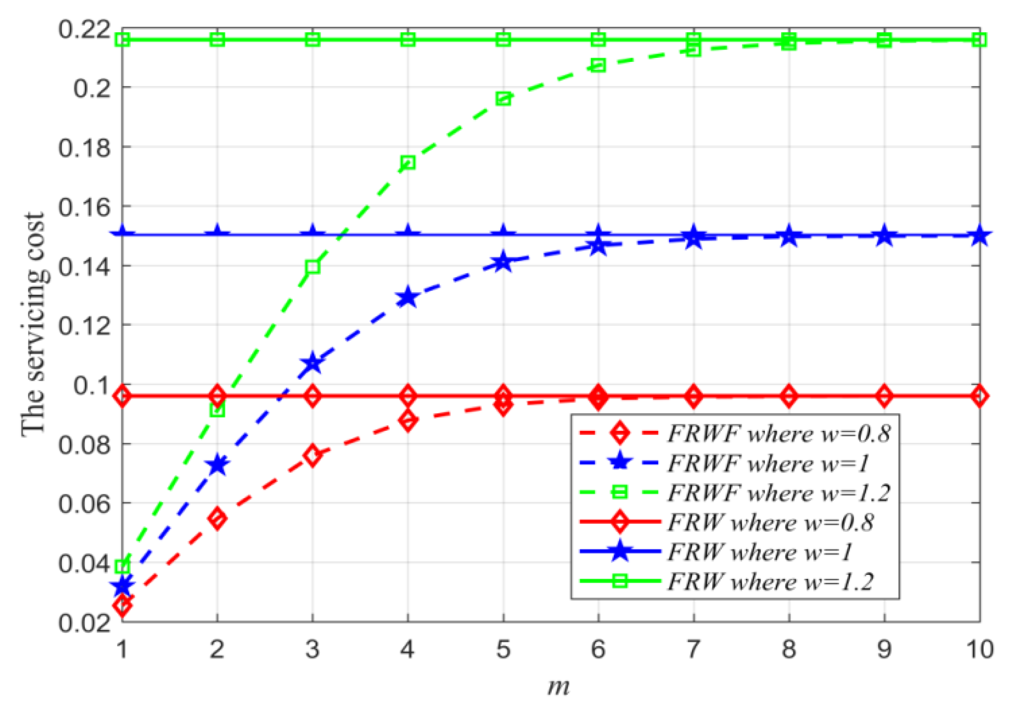
When $\lambda =2$, Figure 1 is obtained to explore how $m$ and $w$ influence the servicing cost of the FRWF and what relationship exists between the servicing costs of the FRWF and the classic FRW.

As shown in Figure 1, ① for a given $w$, when $m$ increases, the servicing cost of the FRW increases to the servicing cost of the classic FRW. A valuable result can be inferred from this change, namely, a limited $m$ as a term can reduce the servicing cost of the classic FRW, which verifies the conclusion in Equation (5); from the numerical perspective, ② for a given smaller $m$, when $w$ increases, the servicing costs of the FRWF and the classic FRW increase because increasing $w$ can enlarge the region of the warranty service.

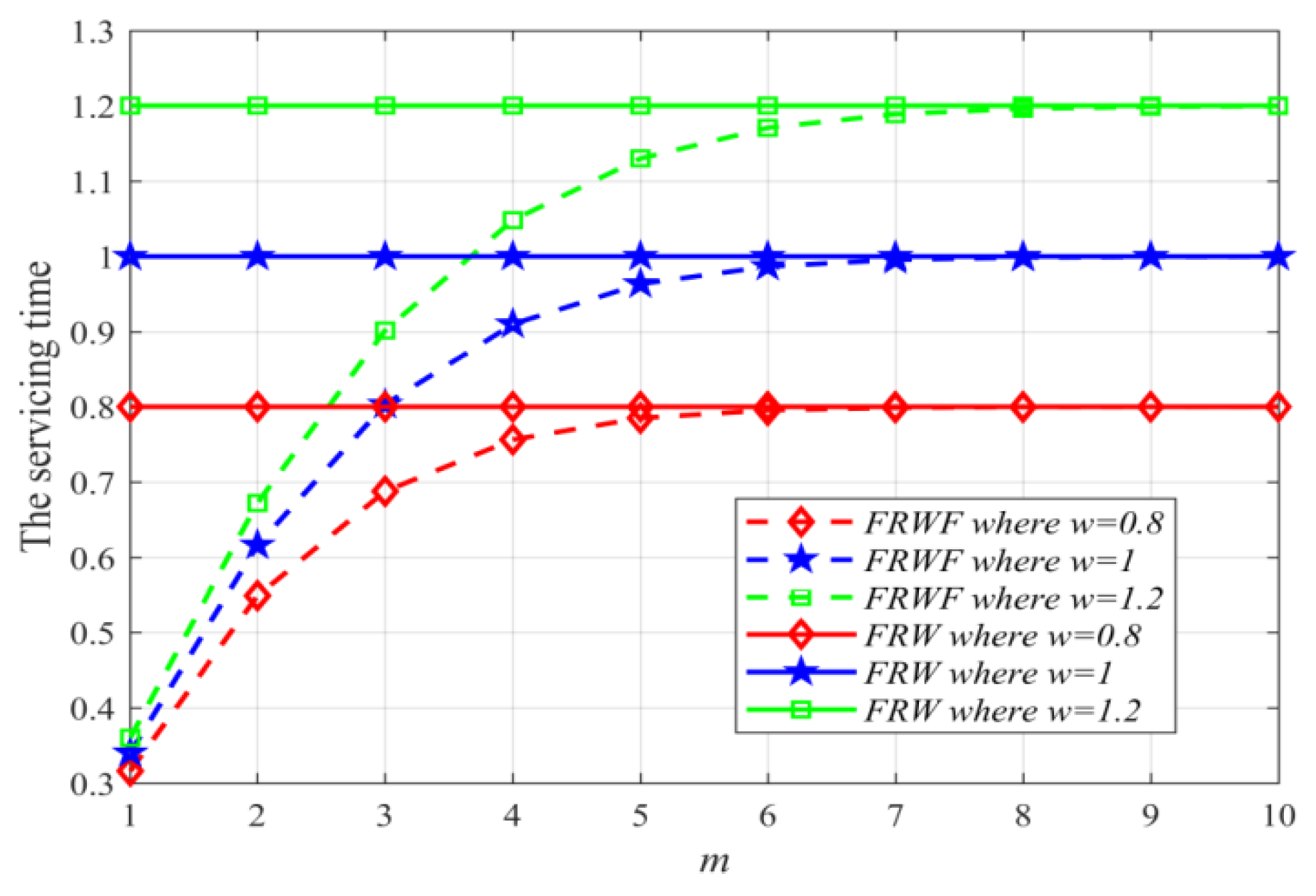
When $\lambda =2$, Figure 2 explores how $m$ and $w$ influence the servicing time of the FRWF and what relationship exists between the servicing times of the FRWF and the classic FRW. Figure 2 shows that ① for a given $w$, $m$ makes the servicing time of the FRWF increase to the servicing time of the classic FRW, and the valuable result is that a limited $m$ can shorten the servicing time of the classic FRW, which verifies the conclusion in Equation (11); ② for a given smaller $m$, $w$ makes the servicing times of the FRWF and the classic FRW increase because the increasing $w$ enlarges the region of the warranty service.

The two results inferred above indicate that, from the numerical perspective, the cost of the warranty service is reduced while its servicing time is shortened. These results signal that the FRWF cannot help the classic FRW to realize the key objective of reducing cost and lengthening time, which cannot illustrate the performance relationship between the FRWF and the classic FRW. To explore the performance relationship of the FRWF and the classic FRW,

Table 1. Comparison of the performances between the FRWF and FRW.

$\mathit{m}$	FRWF		FRW		Time Measures		Relationships
	$\mathit{E}\mathit{S}\mathit{C}$	$\mathit{E}\mathit{S}\mathit{T}$	$\underset{\mathit{m}\to \mathit{\infty }}{\mathbf{lim}}\mathit{E}\mathit{S}\mathit{C}$	$\underset{\mathit{m}\to \mathit{\infty }}{\mathbf{lim}}\mathit{E}\mathit{S}\mathit{T}$	$\mathit{T}{\mathit{M}}_{\mathit{F}\mathit{R}\mathit{W}\mathit{F}}$	$\mathit{T}{\mathit{M}}_{\mathit{F}\mathit{R}\mathit{W}}$
1	0.0254	0.3161	0.0960	0.8000	0.0303	0.0203	$T{M}_{FRWF}>T{M}_{FRW}$
2	0.0547	0.5491	0.0960	0.8000	0.0527	0.0438	$T{M}_{FRWF}>T{M}_{FRW}$
3	0.0760	0.6878	0.0960	0.8000	0.0660	0.0608	$T{M}_{FRWF}>T{M}_{FRW}$
4	0.0878	0.7563	0.0960	0.8000	0.0726	0.0702	$T{M}_{FRWF}>T{M}_{FRW}$
5	0.0931	0.7850	0.0960	0.8000	0.0754	0.0745	$T{M}_{FRWF}>T{M}_{FRW}$
6	0.0951	0.7954	0.0960	0.8000	0.0764	0.0761	$T{M}_{FRWF}>T{M}_{FRW}$

is obtained using the numerical method in Section 2.3.

Table 1 shows that ① $T{M}_{FRWF}$ of the FRWF is longer than $T{M}_{FRW}$ of the FRW; ② the increments between $T{M}_{FRWF}$ of the FRWF and $T{M}_{FRW}$ of the FRW decrease as $m$ increases because the increase in $m$ makes the FRWF converge to the FRW (see Equations (5) and (11)). The first result implies that when $m$ is smaller, the performance of the FRW is superior to that of the FRW, which indirectly signals that in the case of $m$ being smaller, the FRW can help the classic FRW realize the two key objectives of reducing cost and lengthening time. In other words, the presented FRWF, where a lower number of job cycles is used, can make manufacturers shoulder lower costs and provide a longer service time for the warranty service.

4.2. Numerical Analysis of the Presented Random Maintenance Strategy

Under the case of the different warranty strategies, four cost rate strategies have been modeled by calculating servicing measures of replacement cycles and computing limits, which correspond to four maintenance strategies, i.e., BCRM, UCRM, CPR, and BRM strategies. In this subsection, only the sensitivities of the UCRM, whose cost rate was derived in Equation (30), are analyzed.

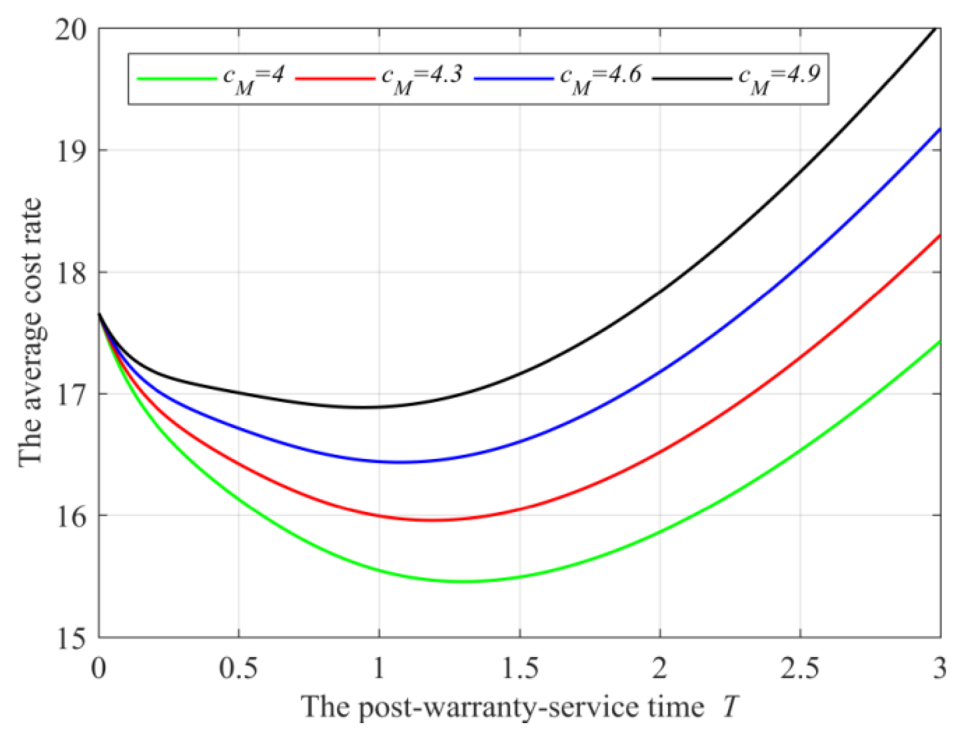
When $c_f=0.1$, $C_{p1}^f=20$, $C_{p2}^f=16$, $C_{p1}^m=15$, $\lambda =2$, $\alpha =1$ and $w=2$, Figure 3 is offered to explore whether the optimal UCRM uniquely exists. Figure 3 shows that ① the optimal post-warranty-servicing time $T^{*}$ and the optimal cost rate $\underset{N\to \infty }{\lim }CR(T^{*},N)$ uniquely exist, which indicates that the optimal UCRM uniquely exists; ② the total cost $c_M$ has a negative effect on the optimal post-warranty-servicing time $T^{*}$ and the optimal cost rate $\underset{N\to \infty }{\lim }CR(T^{*},N)$, which implies that the lower $c_M$ can lengthen the optimal post-warranty-servicing time $T^{*}$ and reduce the optimal cost rate $\underset{N\to \infty }{\lim }CR(T^{*},N)$.

When $c_f=0.1$, $C_{p1}^f=20$, $c_M=0.4$, $C_{p1}^m=15$, $\lambda =2$, $\alpha =1$ and $w=2$,

Table 2. The influences of $m$ and $C_{p2}^f$ on the optimal UCRM.

$\mathit{m}$	${\mathit{C}}_{\mathit{p}2}^{\mathit{f}}=16$		${\mathit{C}}_{\mathit{p}2}^{\mathit{f}}=15$		${\mathit{C}}_{\mathit{p}2}^{\mathit{f}}=14$
	$\underset{\mathit{N}\to \mathit{\infty }}{\mathbf{lim}}\mathit{C}\mathit{R}({\mathit{T}}^{*},\mathit{N})$	${\mathit{T}}^{*}$	$\underset{\mathit{N}\to \mathit{\infty }}{\mathbf{lim}}\mathit{C}\mathit{R}({\mathit{T}}^{*},\mathit{N})$	${\mathit{T}}^{*}$	$\underset{\mathit{N}\to \mathit{\infty }}{\mathbf{lim}}\mathit{C}\mathit{R}({\mathit{T}}^{*},\mathit{N})$	${\mathit{T}}^{*}$
1	5.4080	6.4408	5.3635	6.3852	5.3186	6.3291
2	5.9134	6.8283	5.7996	6.6860	5.6840	6.5416
3	6.3066	7.1185	6.1124	6.8758	5.9147	6.6288
4	6.5241	7.2194	6.2566	6.8851	5.9851	6.5460

is offered to explore the influences of $m$ and $C_{p2}^f$ on the optimal UCRM.

Table 2 shows that ① when the replacement cost $C_{p2}^f$ at the end of the first job cycle is given, the optimal cost rate $\underset{N\to \infty }{\lim }CR(T^{*},N)$ is increasing with respect to $m$, which is suitable for the optimal post-warranty-servicing time $T^{*}$; ② when $m$ is given, the optimal cost rate $\underset{N\to \infty }{\lim }CR(T^{*},N)$ and the optimal post-warranty-servicing time $T^{*}$ are increasing with respect to $C_{p2}^f$. These facts signal that ① when $m$ enlarges the region of the FRWF, the region of the UCRM is extended at the expense of a larger cost rate; ② when $C_{p2}^f$ is larger, the region of the UCRM can be extended at the expense of the larger cost rate.

When $c_f=0.1$, $C_{p1}^f=20$, $C_{p2}^f=16$, $c_M=0.4$, $C_{p2}^m=12$, $\lambda =2$, $\alpha =1$ and $m=2$,

Table 3. The influences of $w$ and $C_{p1}^m$ on the optimal UCRM.

$\mathit{w}$	${\mathit{C}}_{\mathit{p}1}^{\mathit{m}}=15$		${\mathit{C}}_{\mathit{p}1}^{\mathit{m}}=14$		${\mathit{C}}_{\mathit{p}1}^{\mathit{m}}=13$
	$\underset{\mathit{N}\to \mathit{\infty }}{\mathbf{lim}}\mathit{C}\mathit{R}({\mathit{T}}^{*},\mathit{N})$	${\mathit{T}}^{*}$	$\underset{\mathit{N}\to \mathit{\infty }}{\mathbf{lim}}\mathit{C}\mathit{R}({\mathit{T}}^{*},\mathit{N})$	${\mathit{T}}^{*}$	$\underset{\mathit{N}\to \mathit{\infty }}{\mathbf{lim}}\mathit{C}\mathit{R}({\mathit{T}}^{*},\mathit{N})$	${\mathit{T}}^{*}$
1	7.0378	8.3179	6.9348	8.1891	6.8304	8.0587
1.2	6.6839	7.8364	6.5775	7.7035	6.4697	7.5686
1.4	6.4302	7.4957	6.3226	7.3611	6.2133	7.2246
1.6	6.2303	7.2331	6.1225	7.0984	6.0132	6.9617

explores the influences of $w$ and $C_{p1}^m$ on the optimal UCRM. Table 3 shows that ① when the replacement cost $C_{p1}^m$ at post-warranty-servicing time is given, the optimal cost rate $\underset{N\to \infty }{\lim }CR(T^{*},N)$ is decreasing with respect to $w$, which is the same as the optimal post-warranty-servicing time $T^{*}$; ② likewise, when $w$ is given, the optimal cost rate $\underset{N\to \infty }{\lim }CR(T^{*},N)$ and the optimal post-warranty-servicing time $T^{*}$ are increasing with respect to $C_{p1}^m$. These signals indicate that ① when $w$ enlarges the region of the FRWF, the region of the UCRM decreases rather than increases; ② when $C_{p1}^m$ is larger, the region of the UCRM becomes greater at the expense of a greater cost rate.

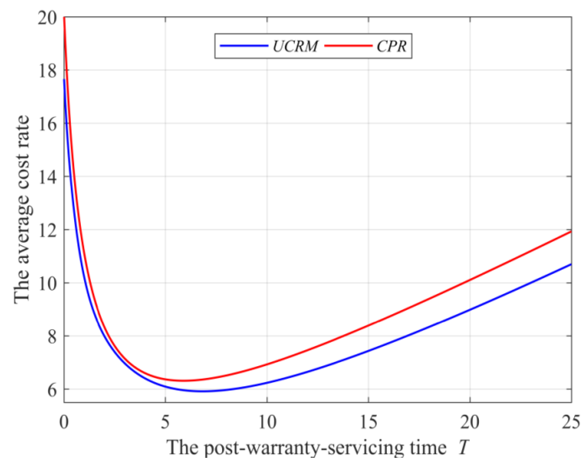
The UCRM strategy has been customized by differing reliabilities, which have been signaled by the ages of FRWF expiries and the differences in the post-warranty reliabilities. From the viewpoint of maintenance theory, the UCRM strategy is an extended model of the classic periodic replacement (CPR) strategy, whose cost rate model has been offered in Equation (31). In view of these relationships, the performance of the UCRM strategy will be explored by taking the CPR strategy as a basic object. Because the optimal strategy has two measures, which are the optimal cost rate and the optimal post-warranty-servicing time, using both to compare the performances is an ideal scheme.

Under the case of $c_f=0.1$, $C_{p1}^f=20$, $C_{p2}^f=16$, $c_M=0.4$, $C_{p1}^m=15$, $C_{p2}^m=13$, $\lambda =2$, $\alpha =1$ and $m=2$, Figure 4 has been plotted to explore the relationships between the optimal cost rates/the optimal post-warranty-servicing times.

Figure 4 shows that the optimal cost rate of the UCRM is lower than the optimal cost rate of the CPR, and the optimal post-warranty-servicing time of the UCRM is longer than the optimal post-warranty-servicing time of the CPR. These results indicate that the UCRM is superior to the CPR.

5. Conclusions

From the statistical perspective, the reliabilities of the same new identical products are not necessarily identical. By differing the reliabilities of the same new identical products, customizing maintenance strategies for using reliability heterogeneity to flexibly ensure life-cycle reliabilities is a novel and practical topic. Under the case of taking products with monitored job cycles as research objects, this paper customized two random maintenance strategies by differing the reliabilities of the same new identical products, which were realized by means of either the designed region or the ages at warranty expiries, or both.

The first strategy is called a flexible repair warranty first (FRWF), which satisfies the following: ① the limited job cycles and the limited period of the warranty service are used to form a region with the performance of screening the differences in the reliabilities, and the key objective is to tailor warranty terms based on the obtained differences in the reliabilities; ② all failures in each region of the warranty service are minimally repaired, the costs of which are completely undertaken by the manufacturers; and ③ ‘whichever occurs first’ is used to define the occurrence relationships between the limited job cycles and the limited period of the warranty service. The time and cost measures of the FRWF strategy are modeled to analytically and numerically compare such a strategy with the classic FRW strategy.

The second strategy is called a customized bivariate random maintenance (BCRM) strategy to ensure post-warranty reliability, the average cost rate of which is obtained by means of the replacement cycle. The average cost rates of the variants of BCRM, such as the univariate customized random maintenance (UCRM) strategy and the classic periodic replacement (CPR) strategy, were obtained by calculating limits. Because the customization principle of the UCRM strategy is the same as the customization principle of the BCRM strategy, the UCRM strategy as a representative was analyzed numerically.

The valuable results shown by numerical analysis include but are not limited to the following:

• The performance of the FRWF is superior to that of the FRW, indirectly signaling that, compared with the classic FRW, the FRWF can realize the two key objectives of reducing cost and lengthening time;
• The decrease in the total cost of the unit failure can lengthen the optimal post-warranty-servicing time and reduce the optimal cost rate; when the replacement cost at the end of the first job cycle is lower, the region of the UCRM can be shrunk, and the cost rate is lowered;
• The performance of the UCRM is superior to that of the CPR strategy.

By screening heterogeneities of reliabilities over the life cycle, this paper defined and modeled a random warranty strategy and random maintenance strategies to ensure post-warranty reliability in order to use the heterogeneities in reliabilities to manage the life-cycle reliability. The heterogeneities in usages and job cycles have substantial effects on the life-cycle reliability, which were ignored in this paper. In addition, the number of failures occurring during the post-warranty stage is one of the key factors measuring post-warranty reliability, which was not considered in this paper. Therefore, considering all types of heterogeneities affecting the life-cycle reliability, designing and modeling other random warranty strategies and random maintenance strategies to ensure post-warranty reliability are very practical topics, and designing and modeling some maintenance strategies considering the number of post-warranty failures is also a practical topic. Both are being carried out by the present authors.