
Mapping and Quantification of Soil Erosion and Sediment Delivery in Poorly Developed Urban Areas: A Case Study


Abstract
:1. Introduction
1.1. Background
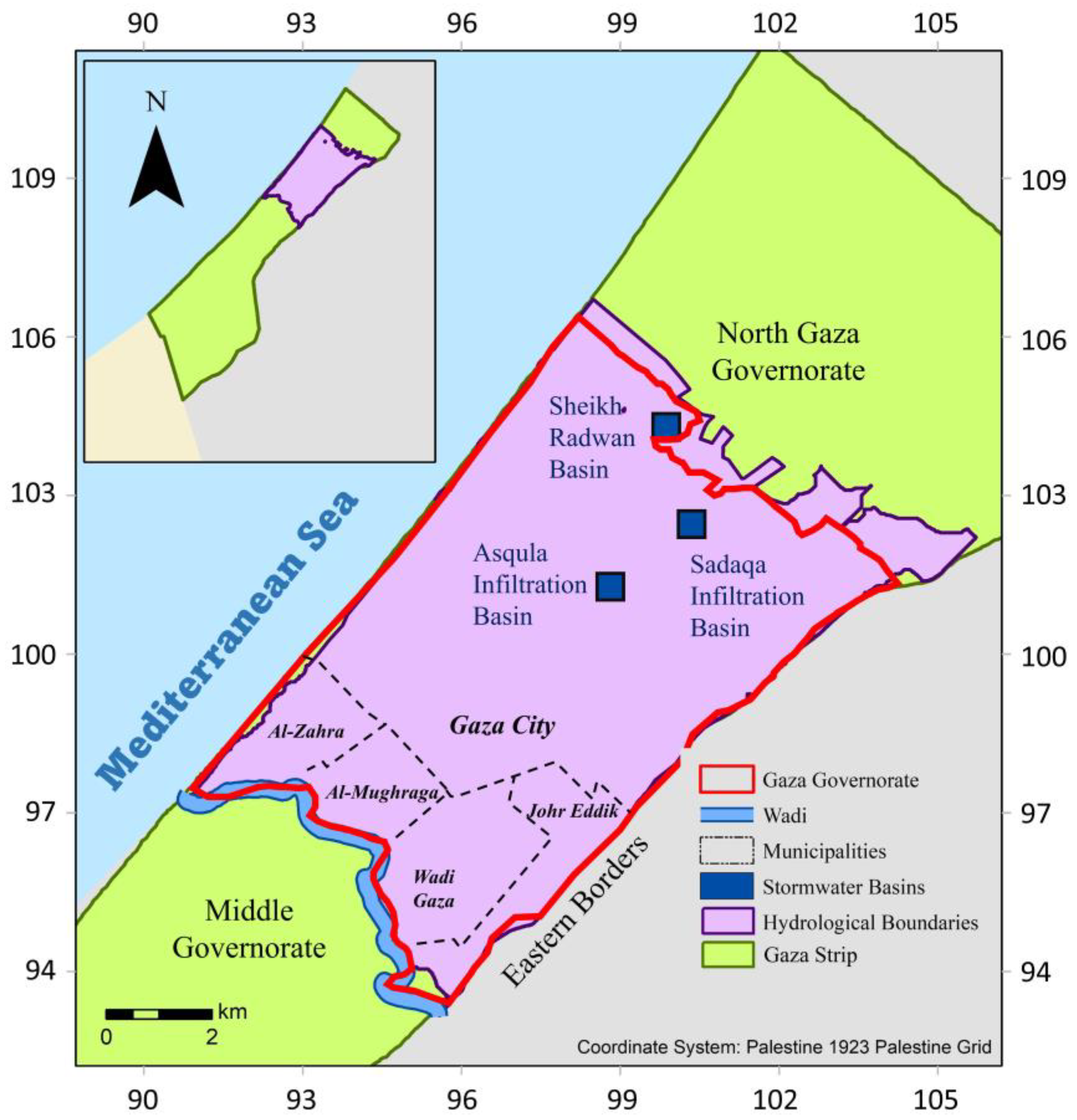
1.2. Study Area
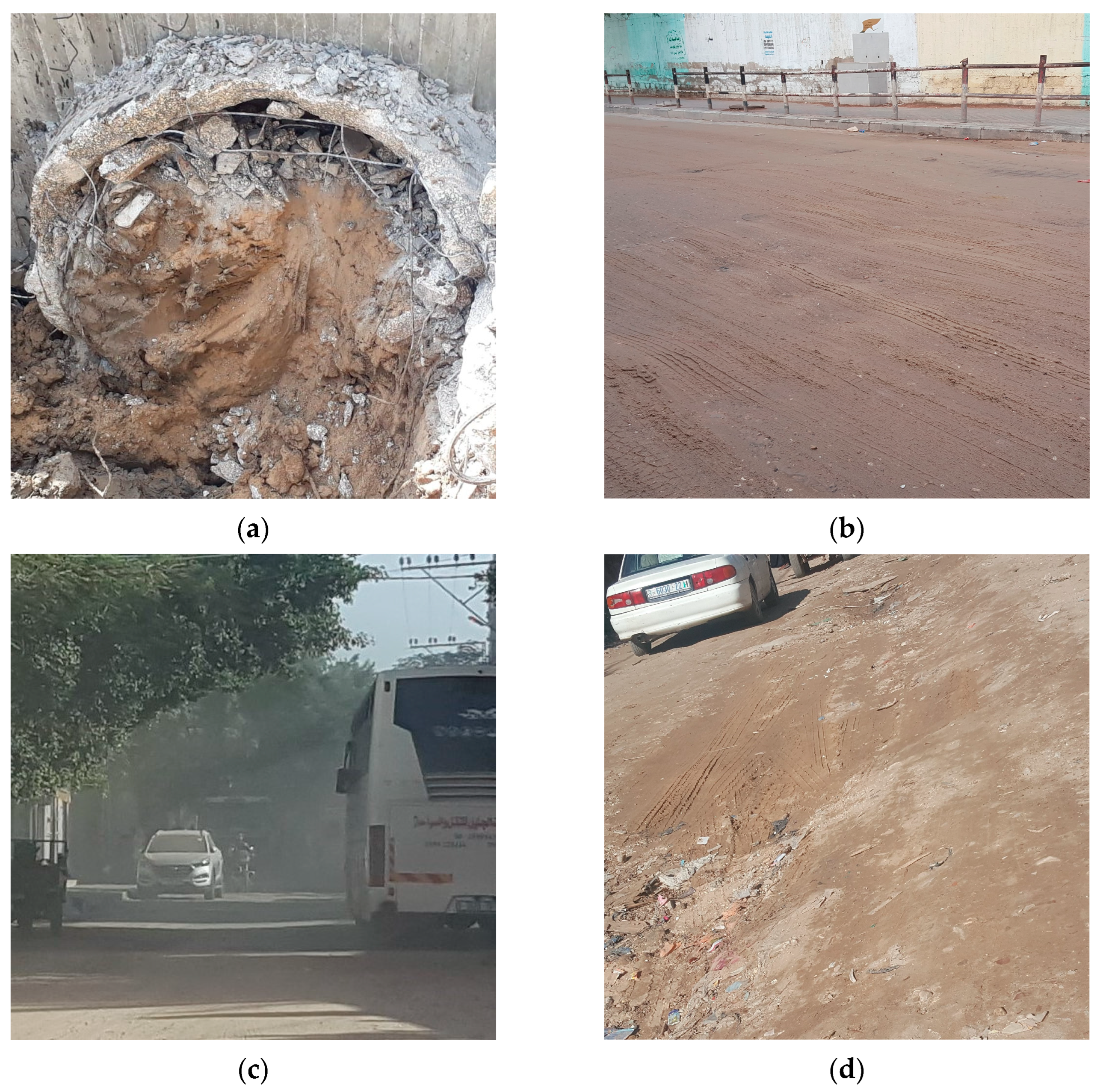
1.3. Problem and Study Motive
1.4. Aims and Objectives
- To compile and filter field data to the highest possible quality and resolution to depict micro-scale geographical variations and to emphasize aspects associated with parameterization of a RUSLE model for the case study location;
- To develop a reasonable calibration model that accounts for stream connectivity in order to enhance the accuracy of the model;
- To describe the urbanization impact on the model results and to highlight any deviations related to the abnormal processes that affected the urbanization structure in the case study;
- To identify regions of high erosion potential and the SDR.
2. Methodology
2.1. Field Measurements and Compilation of Essential Hydrological Data
2.1.1. Field Measurements of Accumulated Sediments
2.1.2. Compilation of the RUSLE Model Data
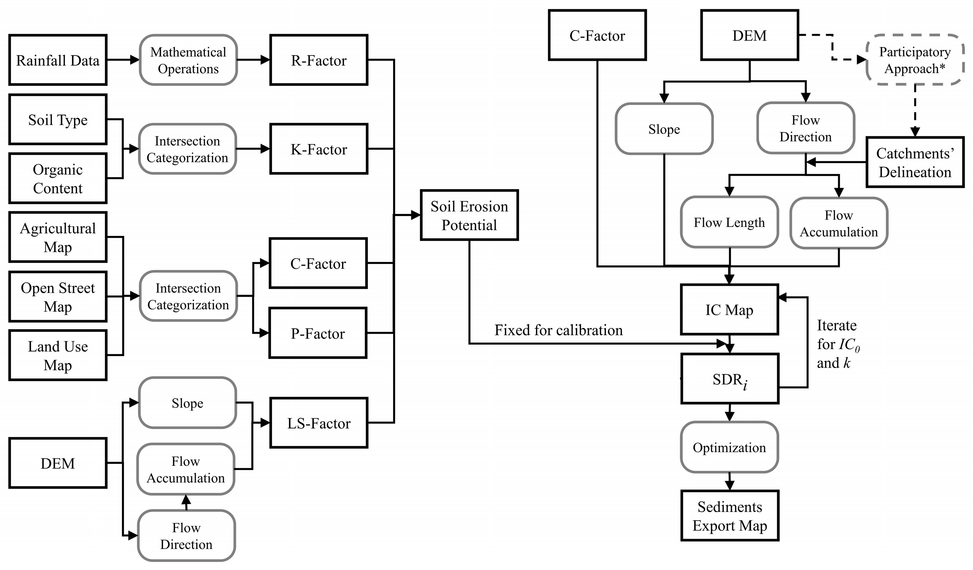
2.2. Soil Loss Model
2.2.1. Revised Universal Soil Loss Equation (RUSLE)
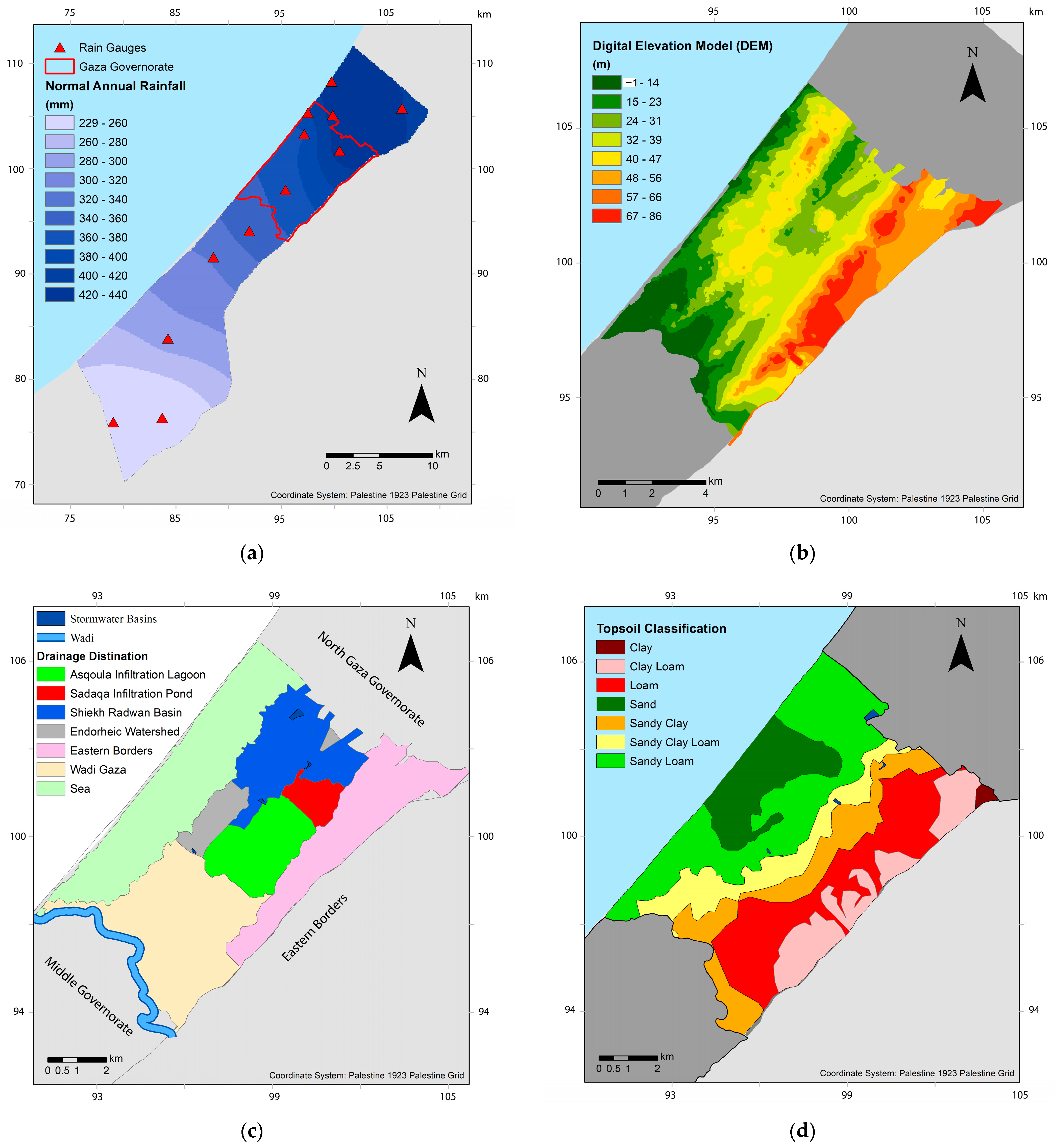
2.2.2. Compilation of Spatial Data and Parameters
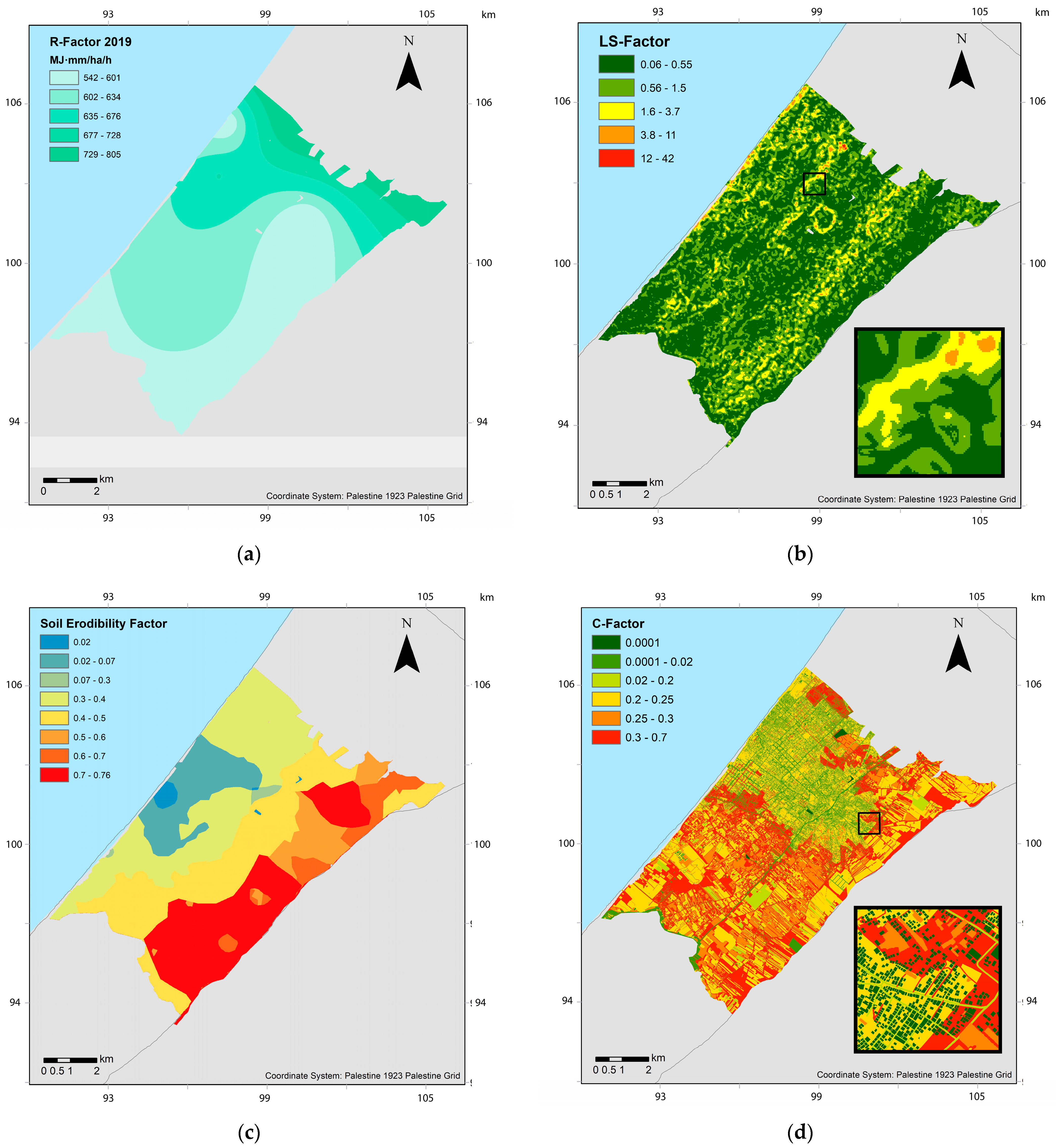
- Rainfall Erosivity Factor (R Factor)
- Soil Erodibility Factor (K Factor)
- Slope Length and Steepness Factor (LS Factor)
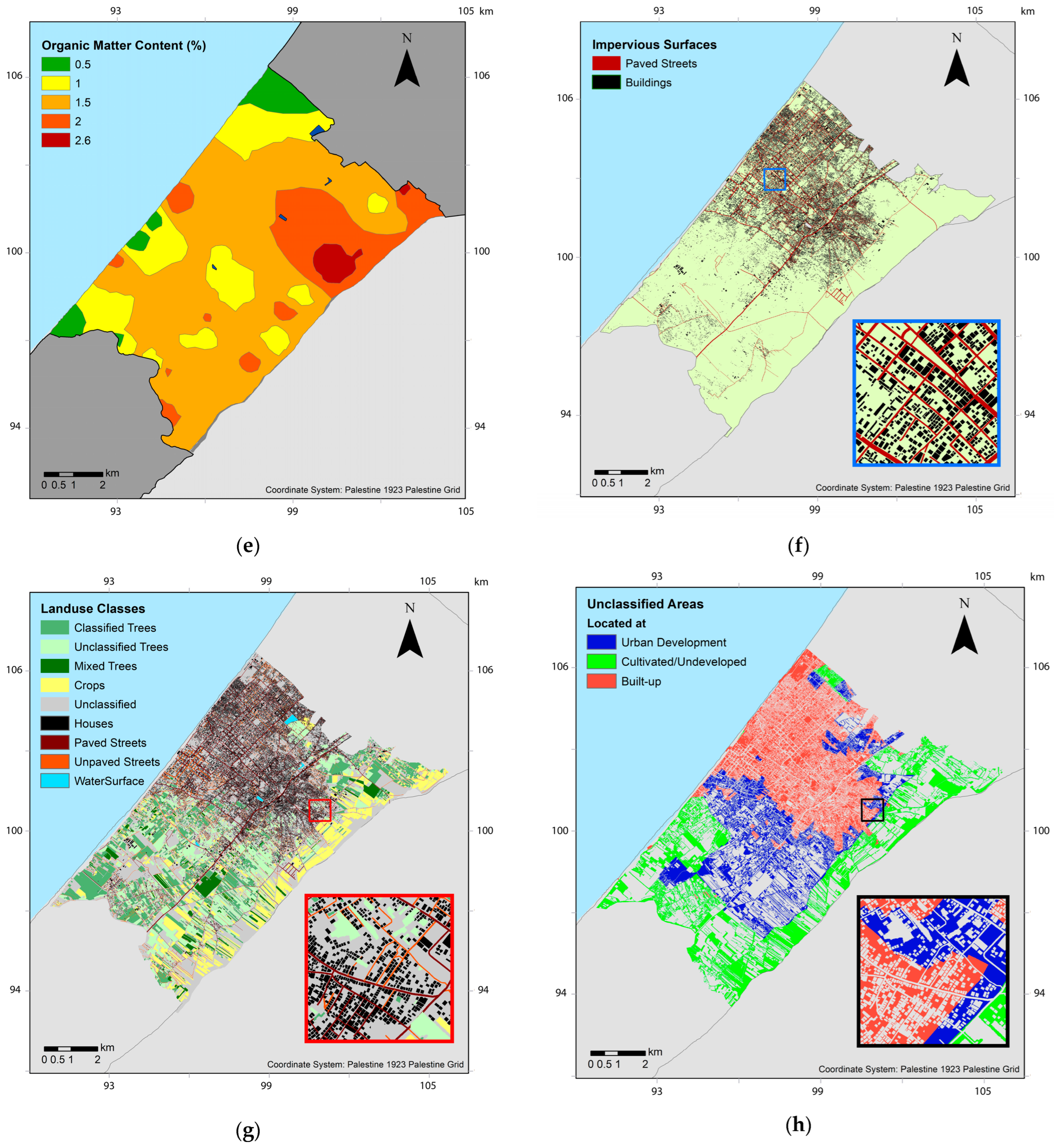
- Cover Management Factor (C Factor)
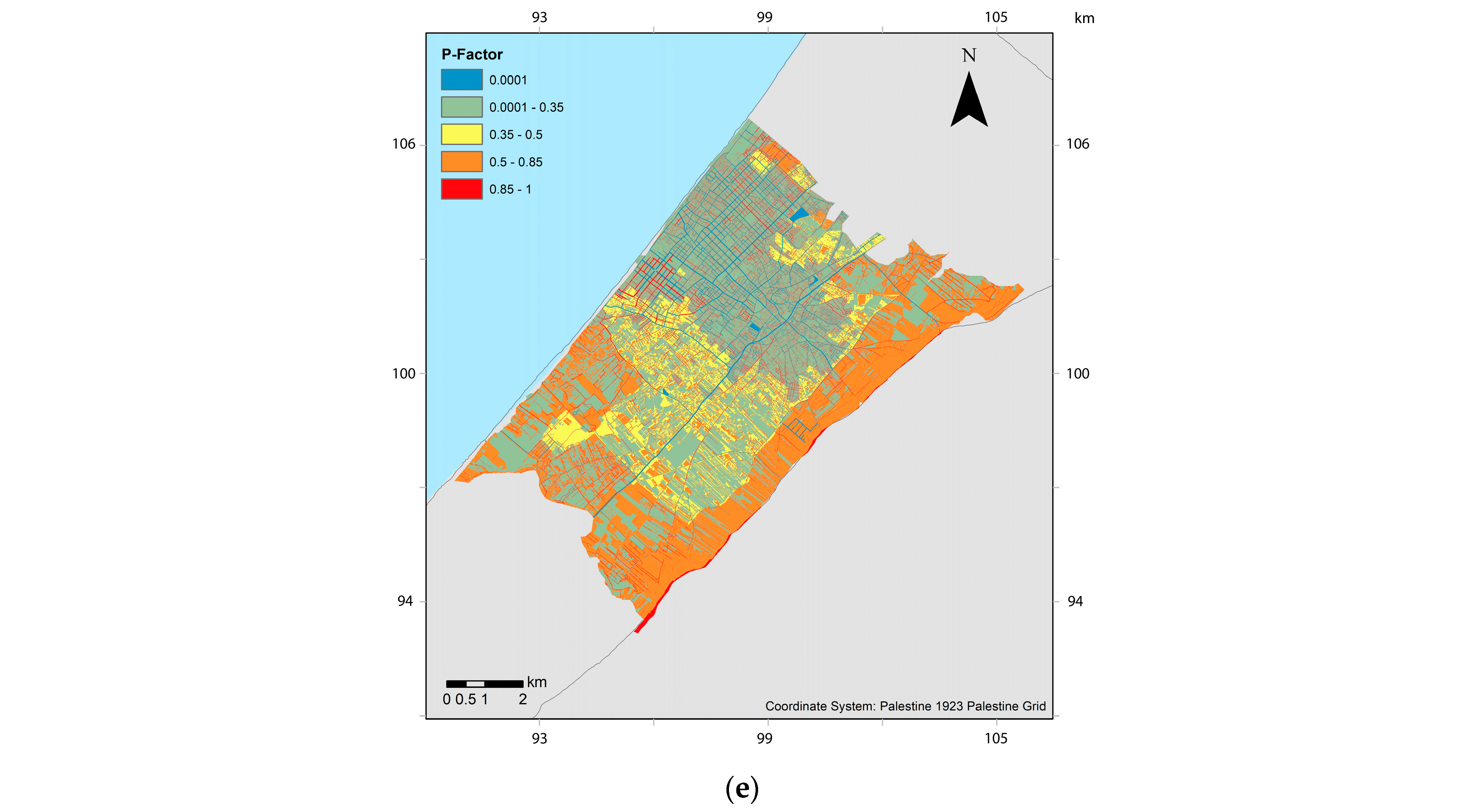
- Erosion Control Practice Factor (P Factor)
2.3. Sediment Delivery Ratio and Calibration of the Model
3. Results
3.1. RUSLE Parameters
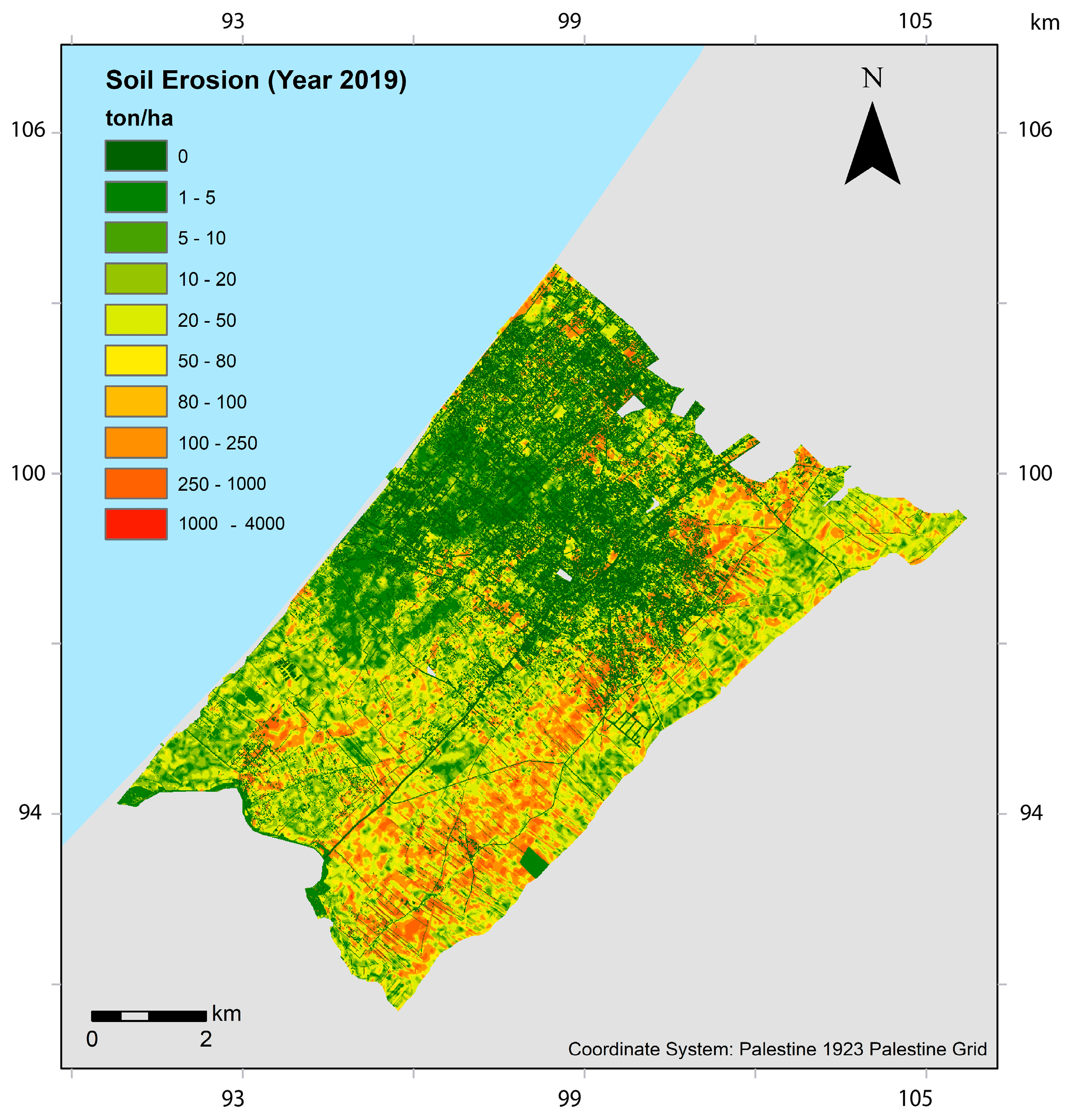
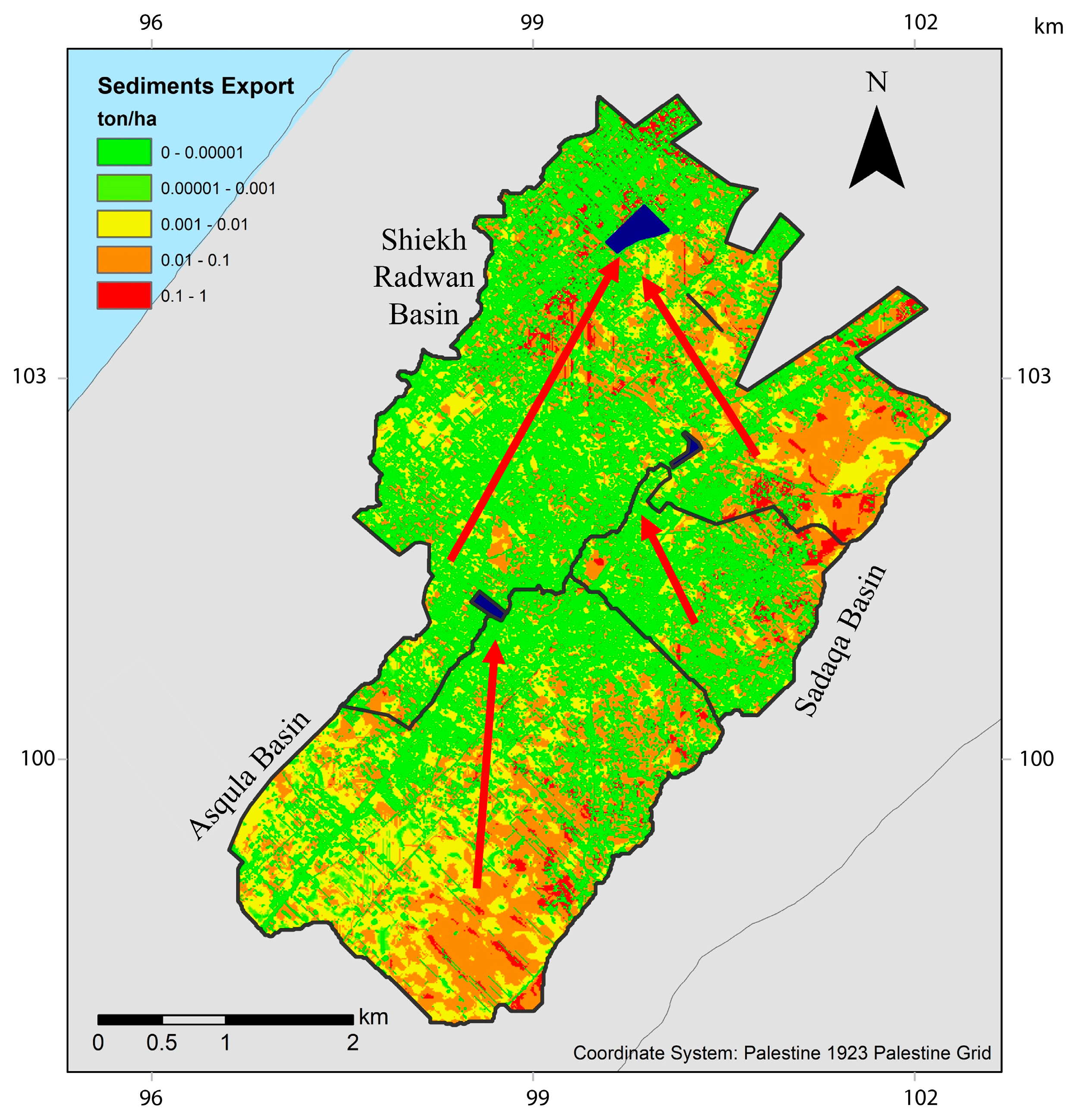
3.2. Sediment Generation Potential
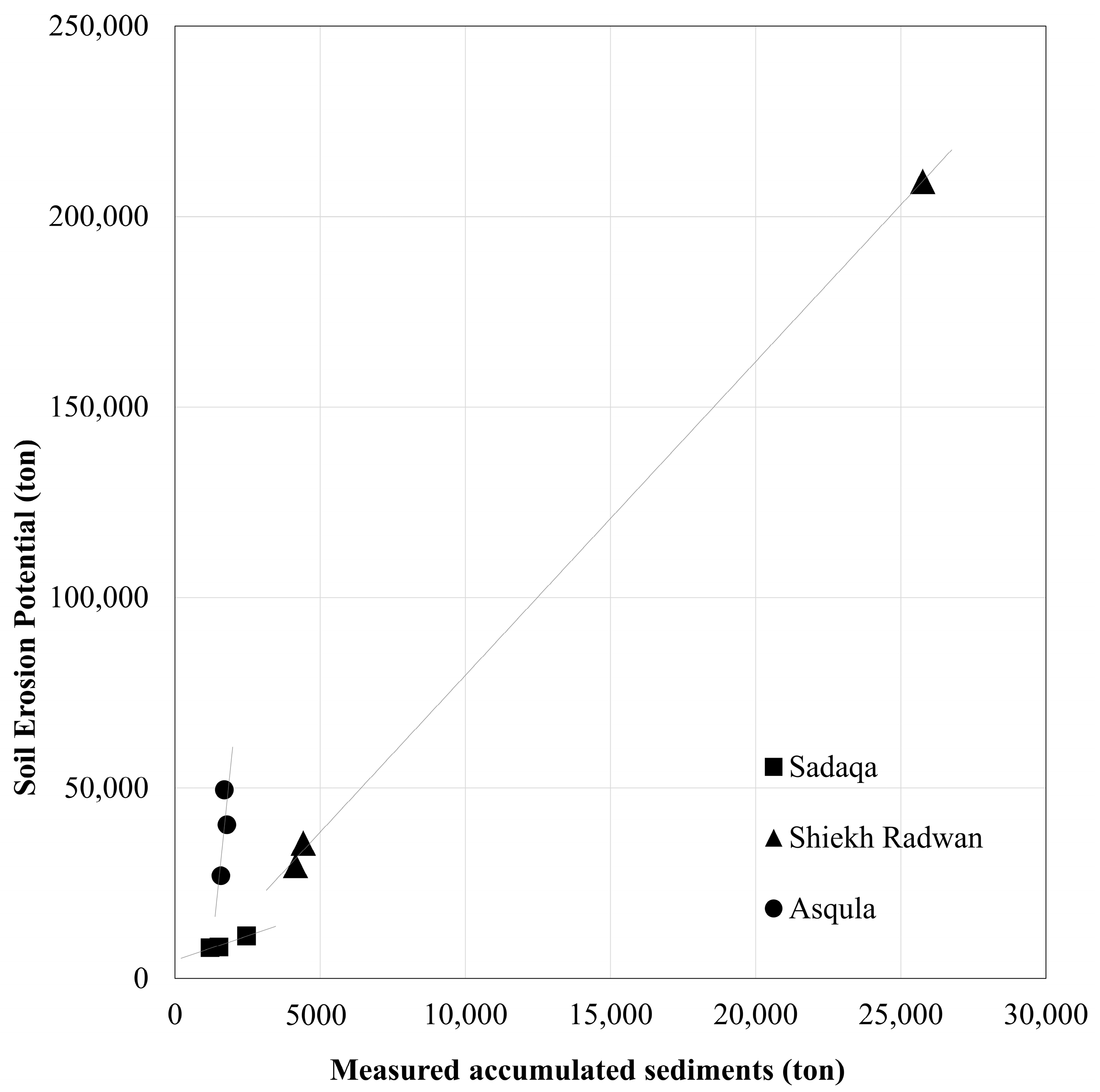
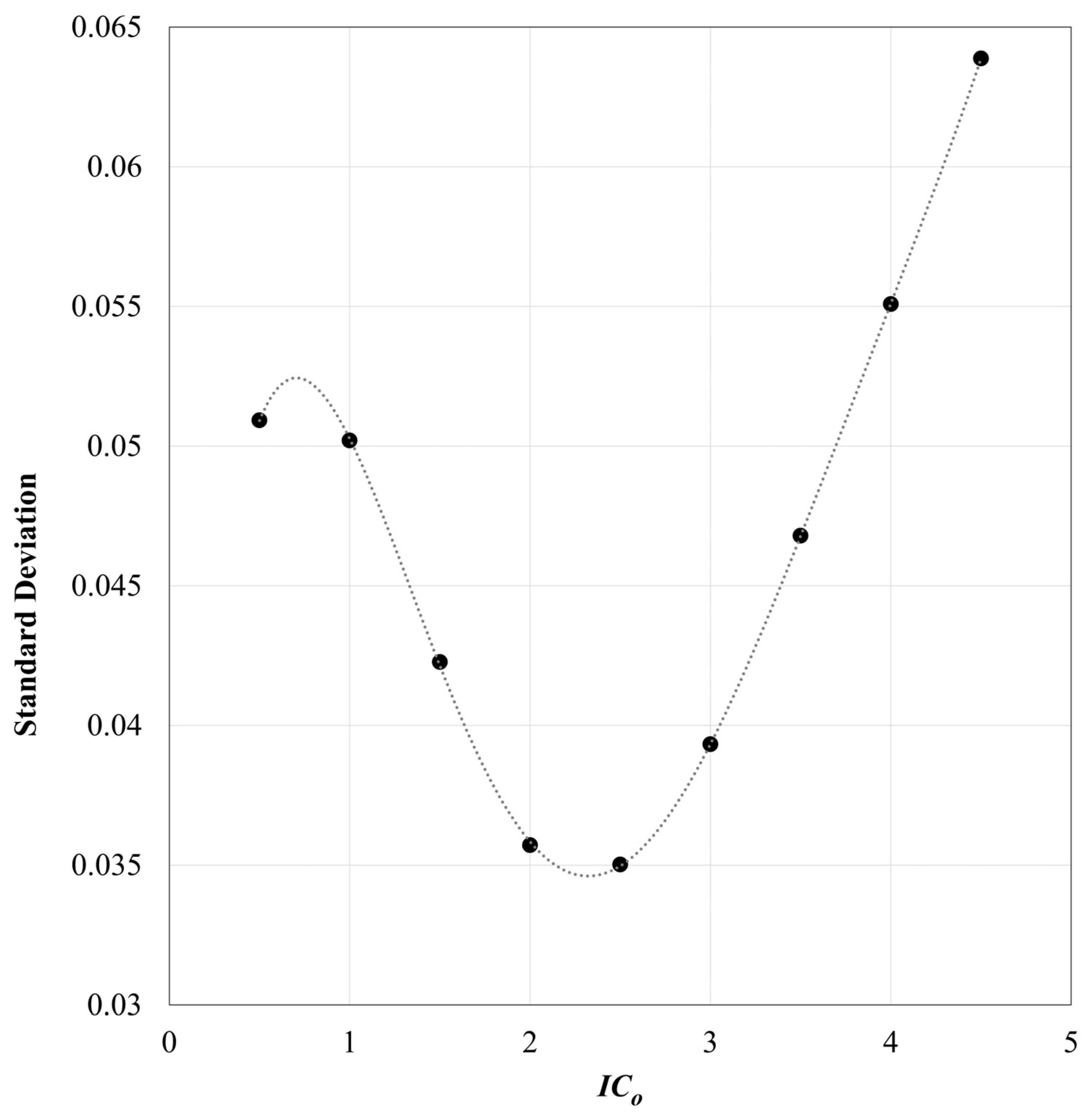
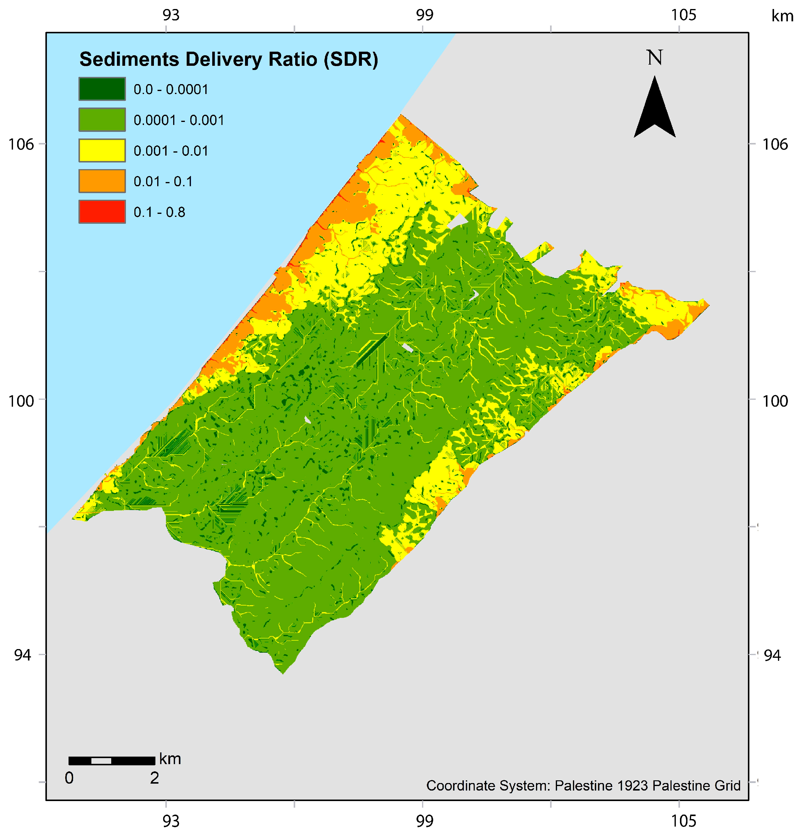
3.3. Sediment Delivery Ratio and Model Calibration and Validation
4. Discussion
5. Conclusions
Author Contributions
Funding
Data Availability Statement
Acknowledgments
Conflicts of Interest
References
- Pandey, S.; Kumar, P.; Zlatic, M.; Nautiyal, R.; Panwar, V.P. Recent advances in assessment of soil erosion vulnerability in a watershed. Int. Soil Water Conserv. Res. 2021, 9, 305–318. [Google Scholar] [CrossRef]
- Wischmeier, W.H.; Smith, D.D. Predicting Railfall Erosion Losses: A Guide to Conservation Planning; United States Department of Agriculture: Washington, DC, USA, 1978. [Google Scholar]
- Renard, K.G.; Freimund, J.R. Using monthly precipitation data to estimate the R-factor in the revised USLE. J. Hydrol. 1994, 157, 287–306. [Google Scholar] [CrossRef]
- Guy, H.P. Sediment Problems in Urban Areas; USGS Numbered Series 601-E; U.S. Geological Survey: Reston, VA, USA, 1970. [Google Scholar] [CrossRef]
- Zhao, H.; Li, X.; Wang, X.; Tian, D. Grain size distribution of road-deposited sediment and its contribution to heavy metal pollution in urban runoff in Beijing, China. J. Hazard. Mater. 2010, 183, 203–210. [Google Scholar] [CrossRef]
- Ferreira, C.S.S.; Walsh, R.P.D.; Ferreira, A.J.D. Degradation in urban areas. Curr. Opin. Environ. Sci. Health 2018, 5, 19–25. [Google Scholar] [CrossRef]
- Rossi, L.; Chèvre, N.; Fankhauser, R.; Margot, J.; Curdy, R.; Babut, M.; Barry, D.A. Sediment contamination assessment in urban areas based on total suspended solids. Water Res. 2013, 47, 339–350. [Google Scholar] [CrossRef]
- Müller, A.; Österlund, H.; Marsalek, J.; Viklander, M. The pollution conveyed by urban runoff: A review of sources. Sci. Total. Environ. 2020, 709, 136125. [Google Scholar] [CrossRef]
- Conley, G.; Beck, N.; Riihimaki, C.A.; Tanner, M. Quantifying clogging patterns of infiltration systems to improve urban stormwater pollution reduction estimates. Water Res. X 2020, 7, 100049. [Google Scholar] [CrossRef]
- Renard, K.G.; Foster, G.R.; Weesies, G.A.; McCool, D.K.; Yoder, D.C. (Eds.) Predicting soil erosion by water: A guide to conservation planning with the revised universal soil loss equation (RUSLE). In Agriculture Handbook, No. 703; US Department of Agriculture, Agricultural Research Service: Washington, DC, USA, 1997. [Google Scholar]
- Borrelli, P.; Alewell, C.; Alvarez, P.; Anache, J.A.A.; Baartman, J.; Ballabio, C.; Bezak, N.; Biddoccu, M.; Cerdà, A.; Chalise, D.; et al. Soil erosion modelling: A global review and statistical analysis. Sci. Total. Environ. 2021, 780, 146494. [Google Scholar] [CrossRef]
- Rahaman, S.A.; Aruchamy, S.; Jegankumar, R.; Ajeez, S.A. Estimation of Annual Average Soil Loss, Based on Rusle Model in Kallar Watershed, Bhavani Basin, Tamil Nadu, India. In ISPRS Annals of the Photogrammetry, Remote Sensing and Spatial Information Sciences; Copernicus GmbH: Kuala Lumpur, Malaysia, 2015; pp. 207–214. [Google Scholar] [CrossRef]
- Balasubramani, K.; Veena, M.; Kumaraswamy, K.; Saravanabavan, V. Estimation of soil erosion in a semi-arid watershed of Tamil Nadu (India) using revised universal soil loss equation (rusle) model through GIS. Model. Earth Syst. Environ. 2015, 1, 10. [Google Scholar] [CrossRef]
- Mihi, A.; Benarfa, N.; Arar, A. Assessing and mapping water erosion-prone areas in northeastern Algeria using analytic hierarchy process, USLE/RUSLE equation, GIS, and remote sensing. Appl. Geomat. 2020, 12, 179–191. [Google Scholar] [CrossRef]
- Farhan, Y.; Zregat, D.; Farhan, I. Spatial Estimation of Soil Erosion Risk Using RUSLE Approach, RS, and GIS Techniques: A Case Study of Kufranja Watershed, Northern Jordan. J. Water Resour. Prot. 2013, 5, 1247–1261. [Google Scholar] [CrossRef]
- Ghosal, K.; Das Bhattacharya, S. A Review of RUSLE Model. J. Indian Soc. Remote Sens. 2020, 48, 689–707. [Google Scholar] [CrossRef]
- Fang, G.; Yuan, T.; Zhang, Y.; Wen, X.; Lin, R. Integrated study on soil erosion using RUSLE and GIS in Yangtze River Basin of Jiangsu Province (China). Arab. J. Geosci. 2019, 12, 173. [Google Scholar] [CrossRef]
- Qi, X.; Li, Q.; Yue, Y.; Liao, C.; Zhai, L.; Zhang, X.; Wang, K.; Zhang, C.; Zhang, M.; Xiong, Y. Rural–Urban Migration and Conservation Drive the Ecosystem Services Improvement in China Karst: A Case Study of HuanJiang County, Guangxi. Remote Sens. 2021, 13, 566. [Google Scholar] [CrossRef]
- Michalek, A.; Zarnaghsh, A.; Husic, A. Modeling linkages between erosion and connectivity in an urbanizing landscape. Sci. Total. Environ. 2021, 764, 144255. [Google Scholar] [CrossRef]
- AAH. Flood-Risk Mitigation Plan for Gaza Strip; Action Against Hunger: Gaza, Palestine, 2018. [Google Scholar]
- PCBS. Palestinian Central Bureau of Statistics (PCBS). 2020. Available online: http://www.pcbs.gov.ps/ (accessed on 25 August 2020).
- Dawoud, O.; Ahmed, T.; Abdel-Latif, M.; Abunada, Z. A spatial multi-criteria analysis approach for planning and management of community-scale desalination plants. Desalination 2020, 485, 114426. [Google Scholar] [CrossRef]
- Podda, A.; Cavazza, L.; Fadda, A.; Vissani, M.; Vascellari, M.; Dawoud, O.; Zoppis, R. Blending between desalinated water and other sources. Desalination Water Treat. 2018, 102, 76–81. [Google Scholar] [CrossRef]
- Russell, K.L.; Vietz, G.J.; Fletcher, T.D. Global sediment yields from urban and urbanizing watersheds. Earth Sci. Rev. 2017, 168, 73–80. [Google Scholar] [CrossRef]
- OpenStreetMap Contributors. Planet Dump. 2020. Available online: https://planet.osm.org (accessed on 23 August 2022).
- MoA. Agriculture Atlas; Geographic Information Systems (GIS) Unit, General Administration for Planning and Policies, Ministry of Agriculture: Gaza, Palestine, 2020. [Google Scholar]
- Dawoud, O.; Mansour, M. A participatory approach for identification of micro flood zones in poorly developed urban areas. In Proceedings of the 4th International Symposium on Natural Hazards (ISHAD2020), Bursa, Turkey, 24–25 October 2020; pp. 941–949. [Google Scholar] [CrossRef]
- Abu Samra, S.A. Determination of Physico-Chemical Properties of Top Soil in Gaza Strip for Agricultural Purposes. Master’s Thesis, Islamic University of Gaza, Gaza, Palestine, 2014. [Google Scholar]
- Schmitt, L.K. Developing and applying a soil erosion model in a data-poor context to an island in the rural Philippines. Environ. Dev. Sustain. 2009, 11, 19–42. [Google Scholar] [CrossRef]
- Kouli, M.; Vallianatos, F.; Soupios, P.; Alexakis, D. GIS-based morphometric analysis of two major watersheds, western Crete, Greece. J. Environ. Hydrol. 2007, 15, 1–17. [Google Scholar]
- Morgan, R.; Quinton, J.N.; Smith, R.E.; Govers, G.; Poesen, J.W.; Auerswald, K.; Folly, A.J. The European Soil Erosion Model (EUROSEM): Documentation and User Guide; Silsoe College, Cranfield University: Cranfield, UK, 1998. [Google Scholar]
- Panagos, P.; Borrelli, P.; Meusburger, K.; Alewell, C.; Lugato, E.; Montanarella, L. Estimating the soil erosion cover-management factor at the European scale. Land Use Policy 2015, 48, 38–50. [Google Scholar] [CrossRef]
- Panagos, P.; Borrelli, P.; Meusburger, K.; Yu, B.; Klik, A.; Lim, K.J.; Yang, J.E.; Ni, J.; Miao, C.; Chattopadhyay, N.; et al. Global rainfall erosivity assessment based on high-temporal resolution rainfall records. Sci. Rep. 2017, 7, 4175. [Google Scholar] [CrossRef] [PubMed]
- Benavidez, R.; Jackson, B.; Maxwell, D.; Norton, K. A review of the (Revised) Universal Soil Loss Equation ((R)USLE): With a view to increasing its global applicability and improving soil loss estimates. Hydrol. Earth Syst. Sci. 2018, 22, 6059–6086. [Google Scholar] [CrossRef]
- Naipal, V.; Reick, C.; Pongratz, J.; Van Oost, K. Improving the global applicability of the RUSLE model—Adjustment of the topographical and rainfall erosivity factors. Geosci. Model Dev. 2015, 8, 2893–2913. [Google Scholar] [CrossRef]
- Brown, L.C.; Foster, G.R. Storm Erosivity Using Idealized Intensity Distributions. Trans. ASAE 1987, 30, 379–386. [Google Scholar] [CrossRef]
- Peel, M.C.; Finlayson, B.L.; McMahon, T.A. Updated world map of the Köppen-Geiger climate classification. Hydrol. Earth Syst. Sci. 2007, 11, 1633–1644. [Google Scholar] [CrossRef]
- Franke, R. Smooth interpolation of scattered data by local thin plate splines. Comput. Math. Appl. 1982, 8, 273–281. [Google Scholar] [CrossRef]
- Mitáš, L.; Mitášová, H. General variational approach to the interpolation problem. Comput. Math. Appl. 1988, 16, 983–992. [Google Scholar] [CrossRef]
- FAO. Geographic Information Systems in Fisheries Management and Planning. Technical Manual. Food and Agriculture Organization of the United Nations. 2003. Available online: http://www.fao.org/3/Y4816E/y4816e00.htm (accessed on 5 January 2021).
- Stone, R.; Hilborn, D. Universal Soil Loss Equation (USLE). Ontario Ministry of Agriculture, Food and Rural Affairs (OMAFRA). 2015. Available online: http://www.omafra.gov.on.ca/english/engineer/facts/12-051.htm (accessed on 14 January 2021).
- Dumas, P.; Fossey, M. Mapping Potential Soil Erosion in the Pacific Islands. A case study of Efate Island (Vanuatu). In Proceedings of the 11th Pacific Science Inter Congress, Pacific Countries and Their Ocean, Facing Local and Global Changes, Tahiti, French Polynesia, 2–6 March 2009. [Google Scholar]
- Nontananandh, S.; Changnoi, B. Internet GIS, Based on USLE Modeling, for Assessment of Soil Erosion in Songkhram Watershed, Northeastern of Thailand. Agric. Nat. Resour. 2012, 46, 272–282. [Google Scholar]
- Das, S.; Bora, P.K.; Das, R. Estimation of slope length gradient (LS) factor for the sub-watershed areas of Juri River in Tripura. Model. Earth Syst. Environ. 2021, 8, 1171–1177. [Google Scholar] [CrossRef]
- Hrabalíková, M.; Janeček, M. Comparison of different approaches to LS factor calculations based on a measured soil loss under simulated rainfall. Soil Water Res. 2017, 12, 69–77. [Google Scholar] [CrossRef]
- USDA-SCS. ‘Hyrology’ in SCS National Engineering Handbook, Section 4; US Department of Agriculture: Washington, DC, USA, 1972. [Google Scholar]
- Theobald, D.M.; Merritt, D.M.; Norman, J.B. Assessment of Threats to Riparian Ecosystems in the Western US; Colorado State University: Fort Collins, CO, USA, 2010. [Google Scholar]
- Adornado, H.A.; Yoshida, M.; Apolinares, H.A. Erosion Vulnerability Assessment in REINA, Quezon Province, Philippines with Raster-based Tool Built within GIS Environment. Agric. Inf. Res. 2009, 18, 24–31. [Google Scholar] [CrossRef]
- Mattheus, C.; Norton, M. Comparison of pond-sedimentation data with a GIS-based USLE model of sediment yield for a small forested urban watershed. Anthropocene 2013, 2, 89–101. [Google Scholar] [CrossRef]
- Croke, J.; Mockler, S.; Fogarty, P.; Takken, I. Sediment concentration changes in runoff pathways from a forest road network and the resultant spatial pattern of catchment connectivity. Geomorphology 2005, 68, 257–268. [Google Scholar] [CrossRef]
- Borselli, L.; Cassi, P.; Torri, D. Prolegomena to sediment and flow connectivity in the landscape: A GIS and field numerical assessment. CATENA 2008, 75, 268–277. [Google Scholar] [CrossRef]
- Vigiak, O.; Borselli, L.; Newham, L.; McInnes, J.; Roberts, A. Comparison of conceptual landscape metrics to define hillslope-scale sediment delivery ratio. Geomorphology 2012, 138, 74–88. [Google Scholar] [CrossRef]
- Zanandrea, F.; Michel, G.P.; Kobiyama, M.; Censi, G.; Abatti, B.H. Spatial-temporal assessment of water and sediment connectivity through a modified connectivity index in a subtropical mountainous catchment. CATENA 2021, 204, 105380. [Google Scholar] [CrossRef]
- Heckmann, T.; Cavalli, M.; Cerdan, O.; Foerster, S.; Javaux, M.; Lode, E.; Smetanová, A.; Vericat, D.; Brardinoni, F. Indices of sediment connectivity: Opportunities, challenges and limitations. Earth Sci. Rev. 2018, 187, 77–108. [Google Scholar] [CrossRef]
- Wolman, M.G. A Cycle of Sedimentation and Erosion in Urban River Channels. Geogr. Ann. Ser. A Phys. Geogr. 1967, 49, 385–395. [Google Scholar] [CrossRef]


| No. | Stormwater Basin | Measurement Year(s) | Quantity (ton) |
|---|---|---|---|
| 1 | Sheikh Radwan | 2014–2018 | 25,755 |
| 2019 | 4148 | ||
| 2020 | 4420 | ||
| 2 | Asqula | 2018 | 1581 |
| 2019 | 1785 | ||
| 2020 | 1700 | ||
| 3 | Sadaqa | 2017–2018 | 2465 |
| 2019 | 1207 | ||
| 2020 | 1513 |
| Data | Format | Source | Used For |
|---|---|---|---|
| Rainfall data | Monthly records at meteorological stations for the years from 2014 to 2020, in addition to the coordinates of these stations | Periodic Publications of Ministry of Agriculture (MoA) | R factor |
| Land-use data | A digital thematic map converted to a grid of 1 m resolution | Ministry of Planning and Administrative Development (MoPAD) | C, and P factors |
| Building and street map | A digital thematic map converted to a grid of 1 m resolution | Open Street Map Contribution Planet [25] | C, and P factors |
| Agriculture map and crop types | A digital thematic map converted to a grid of 1 m resolution | Agriculture Atlas [26] | C factor |
| DEM | A digital grid of 1 m resolution and a float value for elevation | Interpolated surface from an extensive dataset of field surveyed elevations [22] | LS and connectivity index (IC) |
| Hydrological delineation | A digital thematic map showing the urban hydrological delineation of watersheds in the study area | AAH employed a participatory approach for delineation of the urban watersheds [20,27]. | LS and IC |
| Topsoil classification | A grid digitized into 1 m resolution | [28] | K factor |
| Topsoil organic content | A grid digitized into 1 m resolution | [28] | K factor |
| Field measurements | Records from total sediments removed from stormwater detention basins | Municipality of Gaza Water and Wastewater Management Unit | Calibration and validation of the model |
| Textural Class | Organic Matter | |
|---|---|---|
| <2% | >2% | |
| Sand | 0.07 | 0.02 |
| Sandy loam | 0.31 | 0.27 |
| Sandy clay loam | 0.45 | 0.45 |
| Sandy clay 1 | 0.50 | 0.46 |
| Loam | 0.76 | 0.58 |
| Clay loam | 0.74 | 0.63 |
| Clay | 0.54 | 0.47 |
| Buildings and paved roads 2 | 0 | 0 |
| No. | Land-Use Class | Percentage of Land Cover (%) | C Factor | P Factor | |
|---|---|---|---|---|---|
| 1 | Classified trees | 12.3 | 0.2 | 0.35 | |
| 2 | Unclassified trees | 10.5 | 0.275 | ||
| 3 | Mixed trees | 2.5 | 0.135 | ||
| 4 | Crops | 9.6 | 0.21 | ||
| 5 | Houses | 12.2 | 0.001 | 0.001 | |
| 6 | Paved streets | 4.3 | 0.02 | 0.0001 | |
| 7 | Unpaved streets | 3.3 | 0.7 | 1 | |
| 8 | Water surfaces | 0.1 | 0.0 | 0 | |
| 9 | Unclassified (mixed use) | Built-up | 15.6 | 0.2 | 0.04 |
| 10 | cultivated/undeveloped | 16.7 | 0.7 | 0.85 | |
| 11 | Urban development | 12.9 | 0.5 | 0.45 * | |
| Year | Min | Max | Mean | St. Dev. |
|---|---|---|---|---|
| 2020 | 0 | 4281 | 62 | 108 |
| 2019 | 0 | 2940 | 45 | 78 |
| 2018 | 0 | 1784 | 29 | 50 |
Disclaimer/Publisher’s Note: The statements, opinions and data contained in all publications are solely those of the individual author(s) and contributor(s) and not of MDPI and/or the editor(s). MDPI and/or the editor(s) disclaim responsibility for any injury to people or property resulting from any ideas, methods, instructions or products referred to in the content. |
© 2023 by the authors. Licensee MDPI, Basel, Switzerland. This article is an open access article distributed under the terms and conditions of the Creative Commons Attribution (CC BY) license (https://creativecommons.org/licenses/by/4.0/).
Share and Cite
Dawoud, O.; Eljamassi, A.; Abunada, Z. Mapping and Quantification of Soil Erosion and Sediment Delivery in Poorly Developed Urban Areas: A Case Study. Sustainability 2023, 15, 13683. https://doi.org/10.3390/su151813683
Dawoud O, Eljamassi A, Abunada Z. Mapping and Quantification of Soil Erosion and Sediment Delivery in Poorly Developed Urban Areas: A Case Study. Sustainability. 2023; 15(18):13683. https://doi.org/10.3390/su151813683
Chicago/Turabian StyleDawoud, Osama, Alaeddinne Eljamassi, and Ziyad Abunada. 2023. "Mapping and Quantification of Soil Erosion and Sediment Delivery in Poorly Developed Urban Areas: A Case Study" Sustainability 15, no. 18: 13683. https://doi.org/10.3390/su151813683
APA StyleDawoud, O., Eljamassi, A., & Abunada, Z. (2023). Mapping and Quantification of Soil Erosion and Sediment Delivery in Poorly Developed Urban Areas: A Case Study. Sustainability, 15(18), 13683. https://doi.org/10.3390/su151813683