Improved Deep Reinforcement Learning for Intelligent Traffic Signal Control Using ECA_LSTM Network

Abstract

Reinforcement learning is one of the most widely used methods for traffic signal control, but the method experiences issues with state information explosion, inadequate adaptability to special scenarios, and low security. Therefore, this paper proposes a traffic signal control method based on the efficient channel attention mechanism (ECA-NET), long short-term memory (LSTM), and double Dueling deep Q-network (D3QN), which is EL_D3QN. Firstly, the ECA-NET and LSTM module are included in order to lessen the state space’s design complexity, improve the model’s robustness, and adapt to various emergent scenarios. As a result, the cumulative reward is improved by 27.9%, and the average queue length, average waiting time, and ${\mathrm{C}\mathrm{O}}_2$ emissions are decreased by 15.8%, 22.6%, and 4.1%, respectively. Next, the dynamic phase interval ${\mathrm{t}}_{\mathrm{g}\mathrm{a}\mathrm{p}}$ is employed to enable the model to handle more traffic conditions. Its cumulative reward is increased by 34.2%, and the average queue length, average waiting time, and ${\mathrm{C}\mathrm{O}}_2$ emissions are reduced by 19.8%, 30.1%, and 5.6%. Finally, experiments are carried out using various vehicle circumstances and unique scenarios. In a complex environment, EL_D3QN reduces the average queue length, average waiting time, and ${\mathrm{C}\mathrm{O}}_2$ emissions by at least 13.2%, 20.2%, and 3.2% compared to the four existing methods. EL_D3QN also exhibits good generalization and control performance when exposed to the traffic scenarios of unequal stability and equal stability. Furthermore, even when dealing with unique events like a traffic surge, EL_D3QN maintains significant robustness.

1. Introduction

The need for transportation is growing as urban populations become denser. The government is under enormous strain and faces significant issues due to the limited road resources in cities that cause an imbalance between supply and demand for traffic. For example, a jammed-up traffic situation results in delays and higher fuel usage, both of which negatively impact the economy [1]. Additionally, many harmful gases are released, harming the environment globally and contributing to climate change [2]. Most significantly, there are issues with road traffic safety that cause an increase in accidents [3]. Therefore, using traffic signal control is the most straightforward and efficient approach to reducing traffic congestion and boosting the driving environment [4].

Currently, most cities use the traditional fixed signal timing strategy [5], which switches traffic phases at scheduled times. Due to the complex, dynamic, and uncertain traffic environments, the conventional management approach has limitations. Its deviation from the complex reality of the traffic situation leads to inefficient control. To this end, many researchers are exploring methods that can actively perceive the current dynamic traffic state. The aim is to better determine traffic signal control strategies, which inspired the research work in this paper. Reinforcement learning (RL) has been extensively applied in numerous control situations, including traffic signal control, as artificial intelligence has developed quickly [6]. Compared with traditional methods, reinforcement learning [7] is a continuous interaction between an intelligent body and its environment. The aim is to learn the optimal timing strategy to improve control performance and achieve long-term goals. These methods have achieved some success in the study process [8,9], but they also have drawbacks of their own. For example, issues like the explosion of traffic status information cannot be resolved using the conventional Q-learning technique [10]. In the last decade, with the development of deep learning, researchers have combined the two to form the deep reinforcement learning algorithm (DRL) [11]. The DRL is used to address many real-world application problems. Many researchers are investigating the DRL at present to alleviate the traffic congestion problem. The goal is to decrease vehicle delays as well as to increase the effectiveness of road traffic.

In research on traffic signal control using the DRL, for various traffic circumstances, researchers have used different state information for signal control [12]. We can find from this that single information leads to inefficient control performance. Cumbersome information increases the computational power and complexity of the DRL. Therefore, this paper needs to address improving control performance in a simple state space. Additionally, some research works have used variable phase sequences [13], which can decrease driver satisfaction with road traffic. Also, drivers can have more fatal safety accidents because they are unsure when the current phase ends. In order to decrease the risk of accidents and startup delay issues, a predefined phase sequence and a clear duration of the present phase are adopted in this study. Furthermore, different traffic flow scenarios arise in real traffic, so this paper must take into account how to dynamically adjust the time interval of the current phase’s duration by the level of congestion. On the other hand, certain scenario occurrences like traffic surges can occur in real traffic situations [14]. The control model needs to respond to this situation, coupled with the fact that there is less research literature related to particular scenarios. In order to maintain strong control performance in unique circumstances, this research also needs to study that.

To address this, this paper proposes an adaptive traffic signal control framework with known phase duration and fixed phase sequence to solve the above three problems. This paper’s main contributions are as follows:

• In order to simplify the design of state space, an efficient channel attention mechanism (ECA-NET) is provided for neural networks. It can improve the weight of key state information and enhance the control effect.
• Based on the queue length, estimate the degree of vehicle congestion and dynamically adjust the time interval ${\mathrm{t}}_{\mathrm{g}\mathrm{a}\mathrm{p}}$ for the current phase’s duration. This method is more suited to dynamic conditions and enhances traffic control effectiveness while lowering the probability of risky behavior.
• Combining long short-term memory (LSTM) to address special circumstances like traffic surges. It can improve the model’s robustness and rate of convergence and also provide a theoretical framework for the study of partial observation scenarios.

The other parts are structured as follows: The related work of this study is presented in Section 2. The problem description for the article appears in Section 3. The updated double dueling deep Q-network (D3QN) method can be seen in Section 4. Section 5 describes the experimental plan and provides an analysis of the results. Finally, Section 6 concludes with this paper.

2. Related Work

More and more academics are using the DRL in the field of traffic signal control as a result of its growth. Although these studies have made considerable progress in increasing the effectiveness and performance of signal control, there are still certain issues and constraints. With good performance in a range of traffic circumstances, Liu et al. [15] proposed an adaptive traffic signal timing system that can directly regulate phase duration, specifying four types of information like queue length as state space. An intelligent traffic signal control system with partial vehicle detection was proposed by Zhang et al. [16]. The state space of this system consists of six types of information, including the number of vehicles. Experiments confirmed that it can offer a very potent overall optimization scheme for various traffic flows. The cyclic phase model, put forth by Ibrokhimov et al. [17], increases the network’s adaptability by using the current phase, duration, and bias value of each phase as the state space. Zhao et al. [18] proposed an RL-based cooperative technique for traffic direction and signal control. Its state space consists of vehicle distance, number of vehicles, and turn signals. Experiments verify better performance in terms of queue length and throughput. Liang et al. [19] combined multiple optimization elements to improve the model performance, but their state space processing is inadequate, producing a lot of redundant data and lessening the training effect. Although all of the above models improve control efficiency, an increase in computational power can also be found. The reason for this is the excessive complexity of their state design and processing. Furthermore, real-world state information cannot be acquired as easily as it can in analog modeling software.

The signal light state was incorporated into the state design by Liu et al. [20] before action reward and punishment coefficients were added to control the intelligent body action choice. To overcome the instability of deep Q-networks by using maximum pressure, Wang et al. [21] suggested a traffic light timing optimization approach based on a D3QN, maximum pressure, and self-organizing traffic lights. Savithramma et al. [22] applied reinforcement learning to reduce the delay, combined with gradient boosting regression tree to reduce the state complexity. This method reduces the waiting delay and state space. Lu et al. [23] proposed dueling recurrent double Q network (D3RQN) to lessen the algorithm’s reliance on the state information available at the time. Different state loss scenarios are also studied to verify the robustness of this algorithm. Wang et al. [24] proposed the DRL method based on traffic inference model. They proved that the performance efficiency is better than other algorithms through the validation of real datasets. The method proposed by Han et al. [25] considers pedestrian and waiting time and utilizes multi-process computing. Experiments show that the training efficiency of the model can be improved. Kolat et al. [26] proposed redefining the reward by inserting the standard deviation of four road sections to regulate multi-intelligence traffic lights. The outcomes demonstrate how much the system may be enhanced using this technique. The mentioned models’ phase durations are unknown, and their time intervals are fixed at 3 to 5 s. This approach does not match the actual traffic conditions and also wastes a lot of road resources.

In addition, the application of the DRL also has problems such as low robustness and slow convergence. Zaman et al. [27] proposed a new task offloading framework in mobile edge computing (MEC) using LSTM for user orientation prediction, which outperforms baseline techniques and improves server utilization. Xu et al. [28] proposed an inductive model based on the activation values of reward detection and masking decision-making neurons, which effectively improves the robustness of traffic signal control. An optimization method was suggested by Zhang et al. [29] using CV data as input and DRQN to dynamically modify the signal parameters. The outcomes of this model, according to experiments, are superior to those of the back-pressure model. Zhao et al. [30] combined a deep reinforcement learning network with LSTM to address the problem of overestimation of target Q and insufficient learning from long-term experience. Experimental results show that the performance of this method outperforms DQN in some observational environments. Xu et al. [31] introduced a DRQN-based signal control method for critical junctions in response to the problem of failures occurring at critical nodes. The experimental results verify the effectiveness of the framework. The above research work has been enhanced accordingly, but fewer studies exist for particular scenarios.

For this, this paper suggests a D3QN algorithm based on the ECA-LSTM neural network (EL_D3QN) in the case of a simple state space. The algorithm then adjusts the size of the time interval ${\mathrm{t}}_{\mathrm{g}\mathrm{a}\mathrm{p}}$ in real time according to the queue length to determine the level of congestion, improving the stability, robustness, convergence, and adaptive ability of the control system.

3. Problem Statement

In order to improve traffic control performance, we are searching for a way to dynamically adjust intersection signals and phase durations in real time for normal and unusual cases. A control model is suggested for this purpose to increase road capacity and decrease vehicle waiting time, queue length, and ${\mathrm{C}\mathrm{O}}_2$ emissions. The traffic signal control model for this study is depicted in Figure 1. It is composed of two parts: an intersection environment with cameras and lights, and an agent written in Python. When choosing an action, the agent receives state information from the environment as input. The signal light then executes the chosen action to alter the intersection’s present environment. The reward value is then collected from the environment when the action has been completed, and learning is carried out continually in this loop.

The intersection model developed in this study is a single intersection model with six entry lanes running north–south and four entry lanes running east–west for left-turn, straight, and right-turn lanes, respectively. In the decision-making process, the agent inputs the state and reward into the network to determine the corresponding action value. When the duration of the current phase is over, the duration of the next phase is changed, and the phases are switched in a fixed order. The phase sequence is four phases: north–south straight green, north–south left turn green, east–west straight green, and east–west left turn green. The single intersection model and the phase sequence diagram are shown in Figure 2a,b, respectively.

3.1. Intersection State

According to the literature [32], the position and speed of a vehicle can directly indicate the condition of the road. For this reason, our paper likewise employs the position ${\mathrm{p}}_{\mathrm{i}}$ and speed ${\mathrm{v}}_{\mathrm{i}}$ of a vehicle. Figure 3 shows the road state space design diagram of this paper. Specifically, a frame extracted using simulation software is processed, and the DTSE discrete meshing method is used to divide each coming road into a grid of the same size. Ultimately, a two-dimensional matrix $\mathrm{S}=\{{\mathrm{S}}_{\mathrm{P}},{\mathrm{S}}_{\mathrm{v}}\}$ consisting of position and speed can be obtained in accordance with the traffic network.

In this paper, the length of the intersection model established in SUMO simulation software is 600 m, and a circle is drawn with a radius of 150 m. This area is taken as the area detectable by the camera. Each inlet road is divided into n grids of length 5 m, where n = b/d, b is 150 m, and d is 5 m. There can only be one vehicle in each grid when determining the vehicle position information. If a vehicle is in two grids, the percentage of cars in the grid is used to determine which grid it belongs in. In a grid, a 1 denotes a vehicle, and a 0 denotes the absence of a vehicle. The intersection road’s posted limit in this article is 13.89 m/s. To obtain the final speed information, the speed of each vehicle is divided by the posted speed restriction, resulting in a normalized speed.

3.2. Action Space

The kinds of variable phase sequences that would impair the driver’s judgment are not realistic to take into account. In this paper, we select the fixed-phase sequence NSG-NSLG-EWG-EWLG, and the action is defined as the traffic signal duration. The set of the action space is $\mathrm{A}=\{\mathrm{0,1},\mathrm{2,3},\mathrm{4,5},\mathrm{6,7},\mathrm{8,9},\mathrm{10,11,12}\}$ and contains all the phase durations that can be adopted by the agent. Each decision is made by selecting an action from the set of actions as an output value and selecting the duration corresponding to the decision action as a way to change the signal light. Equation (1), which contains a middle action value, is used to compute the phase green light duration. When the choice action is less than the middle value, the computed duration is reduced by that many seconds relative to the time remaining in the preceding phase. When the decision exceeds the middle value, the computed duration is extended by the appropriate number of seconds relative to the time remaining in the preceding phase. Specifically, the intermediate action value in this paper is 6. The current time is 20 s if the decision is taken with an action of 4.

$$\mathrm{t}\mathrm{i}\mathrm{m}\mathrm{e}={\mathrm{t}\mathrm{i}\mathrm{m}\mathrm{e}}_{\mathrm{b}\mathrm{a}\mathrm{s}\mathrm{e}}+\left(\mathrm{a}\mathrm{c}\mathrm{t}\mathrm{i}\mathrm{o}\mathrm{n}-{\mathrm{a}\mathrm{c}\mathrm{t}\mathrm{i}\mathrm{o}\mathrm{n}}_{\mathrm{m}\mathrm{i}\mathrm{d}\mathrm{d}\mathrm{l}\mathrm{e}}\right)\ast {\mathrm{t}}_{\mathrm{g}\mathrm{a}\mathrm{p}}$$

(1)

$${\mathrm{t}}_{\mathrm{g}\mathrm{a}\mathrm{p}}=\left\{\begin{array}{c} 5, {\displaystyle \sum _{\mathrm{i}\in \mathrm{I}\mathrm{N}}}{\mathrm{q}\mathrm{u}\mathrm{e}\mathrm{u}\mathrm{e}}_{\mathrm{i}}>\mathrm{b}\ast \mathrm{lane}/5\\ 4, \mathrm{b}\ast \mathrm{lane}/7.5<{\displaystyle \sum _{\mathrm{i}\in \mathrm{I}\mathrm{N}}}{\mathrm{q}\mathrm{u}\mathrm{e}\mathrm{u}\mathrm{e}}_{\mathrm{i}}\le \mathrm{b}\ast \mathrm{lane}/5\\ 3, \mathrm{other}\end{array}\right.$$

(2)

In the above equation, ${\mathrm{t}\mathrm{i}\mathrm{m}\mathrm{e}}_{\mathrm{b}\mathrm{a}\mathrm{s}\mathrm{e}}$ is the base time which is set as 30 s here. ${\mathrm{a}\mathrm{c}\mathrm{t}\mathrm{i}\mathrm{o}\mathrm{n}}_{\mathrm{m}\mathrm{i}\mathrm{d}\mathrm{d}\mathrm{l}\mathrm{e}}$ is the middle action value, which is set to 6; ${\mathrm{t}}_{\mathrm{g}\mathrm{a}\mathrm{p}}$ is the duration interval value; the length of the road that can be detected by the camera is b. lane is the number of entry lanes of the intersection. And, in this paper, we use the total queue length to judge the degree of congestion and change the value of ${\mathrm{t}}_{\mathrm{g}\mathrm{a}\mathrm{p}}$, as shown in Equation (2). ${\mathrm{t}}_{\mathrm{g}\mathrm{a}\mathrm{p}}$ is 3 s if the traffic road is slightly busy. ${\mathrm{t}}_{\mathrm{g}\mathrm{a}\mathrm{p}}$ is 4 s in a moderately busy situation. ${\mathrm{t}}_{\mathrm{g}\mathrm{a}\mathrm{p}}$ is 5 s if there is a lot of congestion. The adjustment can be adapted to more traffic environments and also can be adapted to different intersection models.

When the traffic volume increases, the phase duration continues to grow. To avoid this, set the maximum green light duration and the minimum green light duration for each phase as ${\mathrm{t}}_{\mathrm{m}\mathrm{a}\mathrm{x}}$ = 60 s and ${\mathrm{t}}_{\mathrm{m}\mathrm{i}\mathrm{n}}$ = 10 s, respectively. Once the green light duration of a phase is longer than 60, the maximum duration is directly selected. Less than 10 s, the minimum duration is selected, and a super large negative reward is given to the current action.

3.3. Reward

In traffic signal control, there are many reward and punishment functions. Most researchers construct the reward and punishment functions following the delay time, but in practice, it is challenging to acquire the delay time of vehicles. The agent can be correctly guided by a suitable reward function to learn and adopt the best course of action. This study defines the reward function as the difference between the total waiting periods for two moments. The ultimate objective is to increase road capacity while maximizing the cumulative reward, decreasing average wait time, average queue length, and ${\mathrm{C}\mathrm{O}}_2$ emissions.

The following equation is used to determine the difference between the import lane vehicle’s wait time at the previous and current instants:

$${\mathrm{W}\mathrm{a}\mathrm{i}\mathrm{t}\mathrm{t}\mathrm{i}\mathrm{m}\mathrm{e}}_{\mathrm{t}}=\sum _{\mathrm{i}\in \mathrm{I}\mathrm{N}}{\mathrm{w}\mathrm{a}\mathrm{i}\mathrm{t}\mathrm{t}\mathrm{i}\mathrm{m}\mathrm{e}}_{\mathrm{i}}$$

(3)

$${\mathrm{R}}_{{\mathrm{w}\mathrm{a}\mathrm{i}\mathrm{t}\mathrm{t}\mathrm{i}\mathrm{m}\mathrm{e}}_{\mathrm{t}}}={\mathrm{W}\mathrm{a}\mathrm{i}\mathrm{t}\mathrm{t}\mathrm{i}\mathrm{m}\mathrm{e}}_{\mathrm{t}-1}-{\mathrm{W}\mathrm{a}\mathrm{i}\mathrm{t}\mathrm{t}\mathrm{i}\mathrm{m}\mathrm{e}}_{\mathrm{t}}$$

(4)

The final reward function is:

$$\mathrm{R}={\mathrm{R}}_{{\mathrm{w}\mathrm{a}\mathrm{i}\mathrm{t}\mathrm{t}\mathrm{i}\mathrm{m}\mathrm{e}}_{\mathrm{t}}}$$

(5)

where IN is the number of import lanes, ${\mathrm{w}\mathrm{a}\mathrm{i}\mathrm{t}\mathrm{t}\mathrm{i}\mathrm{m}\mathrm{e}}_{\mathrm{i}}$ is the vehicle waiting time for import lane i, and ${\mathrm{W}\mathrm{a}\mathrm{i}\mathrm{t}\mathrm{t}\mathrm{i}\mathrm{m}\mathrm{e}}_{\mathrm{t}}$ is the total vehicle waiting time for import lanes at the current moment.

3.4. Greedy Strategy

The method presented in this study employs an ε-greedy strategy for decision-making action exploration and exploitation. After acting, the signal light returns a reward value, and the reward value gained each time is saved and calculated before commencing the next iteration. This paper adopts a linearly decaying adaptive exploration factor to balance the link between algorithmic exploration and exploitation, as illustrated in the following equation:

$$\mathsf{\epsilon }=\max \left({\mathsf{\epsilon }}_{\mathrm{e}\mathrm{n}\mathrm{d}},\mathsf{\epsilon }-\frac{{\mathsf{\epsilon }}_{\mathrm{i}\mathrm{n}\mathrm{i}\mathrm{t}}-{\mathsf{\epsilon }}_{\mathrm{e}\mathrm{n}\mathrm{d}}}{{\mathrm{a}\mathrm{n}\mathrm{n}\mathrm{e}\mathrm{l}\mathrm{i}\mathrm{n}\mathrm{g}}_{\mathrm{s}\mathrm{t}\mathrm{e}\mathrm{p}\mathrm{s}}}\right)$$

(6)

In the formula, ${\mathsf{\epsilon }}_{\mathrm{i}\mathrm{n}\mathrm{i}\mathrm{t}}$ is the initial ε, ${\mathsf{\epsilon }}_{\mathrm{e}\mathrm{n}\mathrm{d}}$ is the minimum ε, and ${\mathrm{a}\mathrm{n}\mathrm{n}\mathrm{e}\mathrm{l}\mathrm{i}\mathrm{n}\mathrm{g}}_{\mathrm{s}\mathrm{t}\mathrm{e}\mathrm{p}\mathrm{s}}$ is the decay factor.

4. Improved Double Dueling Deep Q-Network

After establishing the traffic control model, this paper solves the above problem based on the D3QN algorithm. Firstly, the ECA is included in the D3QN network by changing the network’s structure. A complex traffic environment has limited perceptual capabilities, and ECA can automatically focus on critical state components. The aim is to enhance the perception ability of the network and reduce the difficulty of designing the state space. Different weights are assigned to different states, with more weight near the intersection and less weight away from the intersection. Secondly, LSTM is added to the network for two special scenario situations, namely, traffic surge and road capacity limitation. The algorithm EL_D3QN for this paper is then created.

4.1. Neural Network Architecture

The neural network in this research has an architecture made up of two convolutional layers: an ECA layer and an LSTM layer. A vehicle road information matrix of size S∗V∗2, where S∗V is the number of grids in the information matrix and 2 stands for the two attributes of vehicle speed and position, is the input to the network. The data first pass through the first convolutional layer consisting of 32 filters. Each filter is 4 × 4 in size and moves 2 × 2 steps at a time over the entire depth of the input data. Its data output size is 9 × 14 × 32. The second convolutional layer has 64 filters of size 2 × 2 with a step size of 1 × 1 with an output size of 8 × 13 × 64. Since state information cannot be observed in its entirety in reality, the weights of crucial state information must be determined. Next, the output of the second convolutional layer is fed into the ECA to get an 8 × 13 × 64 tensor. Another flattening operation is performed to enter the LSTM layer, and a fully connected layer is used to convert the tensor to a 128 × 1 matrix. Following the first fully connected layer, the data are split into two identically sized (64 × 1) portions. The value is then determined by using the first part, and the benefit by using the second. The size of the final advantage is 13 × 1, which is combined with the obtained values to obtain the Q-value. The neural network architecture is shown in Figure 4.

4.2. ECA-NET

The agent observes the surrounding area to gather the vehicle’s state information. The information is then processed and transmitted to the ECA module for state weight acquisition after processing is completed. This technique can highlight helpful informational elements and gather more precise state data.

As depicted in Figure 5, ECA-NET [33] is a lightweight, improved module based on SENET. In the ECA-NET module, the two fully connected layers of the SENET module are replaced by a one-dimensional convolution with an adaptive kernel size. The goal is to improve the attention of the original model. By adding a small number of parameters, the conflict between model performance and structural complexity is resolved.

ECA converts the input state space into vectors. Next, the adaptive one-dimensional convolution kernel size is calculated based on the number of channels of the feature values. The convolution kernel size is used in the convolution layer to obtain the weights of each channel of the feature map. Then, the output is executed using a sigmoid activation function to keep the channel size constant. The normalized weighted feature map size is stacked with the original input feature map to generate a weighted feature map.

$$\mathsf{\omega }=\mathsf{\sigma }\left(\mathrm{C}1{\mathrm{D}}_{\mathrm{k}}(\mathrm{y})\right)$$

(7)

In Equation (7), $\mathsf{\omega }$ is the channel attention information, $\mathsf{\sigma }$ is the sigmoid activation function, and $\mathrm{C}1\mathrm{D}$ is the one-dimensional convolution. k is the convolution kernel size. y is the output after global average pooling.

$$\mathrm{C}=\mathrm{\varnothing }\left(\mathrm{k}\right)=2^{(\mathsf{\gamma }\ast \mathrm{k}-\mathrm{b})}$$

(8)

C in Equation (8) is the channel dimension, i.e., the number of filters. ∅ is a mapping relation for a nonlinear function. γ and b are parameters.

$$\mathrm{k}=\mathsf{\phi }\left(\mathrm{C}\right)={\left|\frac{{\mathrm{l}\mathrm{o}\mathrm{g}}_2\left(\mathrm{C}\right)}{\mathsf{\gamma }}+\frac{\mathrm{b}}{\mathsf{\gamma }}\right|}_{\mathrm{o}\mathrm{d}\mathrm{d}}$$

(9)

where φ is the mapping relation, the correspondence between the size of the convolution kernel and the number of channels. ${\left|\mathrm{t}\right|}_{\mathrm{o}\mathrm{d}\mathrm{d}}$ denotes the closest odd number of t. In the experiment, γ is 2 and b is 1.

4.3. LSTM

The structure of the LSTM is depicted in Figure 6. It is a distinct recurrent neural network RNN [34] that can analyze the input data using time series to avoid long-term dependency. In particular circumstances, the field of traffic signal control can transform into a partially observable Markov decision that is related to both the historical state and the current state and action. LSTM can encode the historical state information, reducing the model’s reliance on the information about the current state and unlocking certain memory locations.

$${\mathrm{f}}_t=\mathsf{\sigma }\left(W_f·\left[h_{t-1},x_t\right]\right)+b_f$$

(10)

$${\mathrm{i}}_t=\mathsf{\sigma }\left(W_i·\left[h_{t-1},x_t\right]\right)+b_i$$

(11)

$${\mathrm{g}}_t=\mathrm{t}\mathrm{a}\mathrm{n}\mathrm{h}\left(W_C·\left[h_{t-1},x_t\right]\right)+b_C$$

(12)

$${\mathrm{C}}_t={\mathrm{f}}_t\ast {\mathrm{C}}_{t-1}+{\mathrm{i}}_t\ast {\mathrm{g}}_t$$

(13)

$${\mathrm{o}}_t=\mathsf{\sigma }\left(W_o·\left[h_{t-1},x_t\right]\right)+b_o$$

(14)

$${\mathrm{h}}_t={\mathrm{o}}_t\ast \mathrm{t}\mathrm{a}\mathrm{n}\mathrm{h}\left({\mathrm{C}}_t\right)$$

(15)

where t denotes time. $\mathrm{i}$, $\mathrm{f}$, $\mathrm{g}$, and $\mathrm{o}$ denote input, forget, modulation, and output gates, respectively. $x$ is the input, $h$ is the hidden state, $\mathrm{C}$ is the cell state. $W$ and b are parameters. $\mathsf{\sigma }$ is the sigmoid activation function and $\mathrm{t}\mathrm{a}\mathrm{n}\mathrm{h}$ is the $\mathrm{t}\mathrm{a}\mathrm{n}\mathrm{h}$ activation function. $\mathrm{H}\mathrm{a}\mathrm{d}\mathrm{a}\mathrm{m}\mathrm{a}\mathrm{r}\mathrm{d}$ Products are marked with $\ast$.

4.4. Double Dueling Deep Q-Network

The value of the current state and the benefit of each action relative to others are used in the dueling network to estimate Q. The overall predicted benefit of executing a probabilistic action in a subsequent step is represented by the value of state $\mathrm{V}\left(\mathrm{s};\mathsf{\theta }\right)$. The advantage corresponds to each action and is defined as $\mathrm{A}\left(\mathrm{s},\mathrm{a};\mathsf{\theta }\right)$. The value of Q is the sum of the value V and the advantage function A. The value of V and the advantage function A are added to determine the value of Q.

$$\mathrm{Q}\left(\mathrm{s},\mathrm{a};\mathsf{\theta }\right)=\mathrm{V}\left(\mathrm{s};\mathsf{\theta }\right)+(\mathrm{A}\left(\mathrm{s},\mathrm{a};\mathsf{\theta }\right)-\frac{1}{\left|A\right|}\sum _{a^{\prime }}A(s,a^{\prime };\theta ))$$

(16)

$\mathrm{A}\left(\mathrm{s},\mathrm{a};\mathsf{\theta }\right)$ illustrates how significant a certain action is to the value function across all actions. If an action has a positive A-value, it implies that it performs better than the average of all possible actions in terms of numerical rewards. If it has a negative value, it means that the action’s potential reward is lower than the average.

The algorithm has a target network to lessen the policy fluctuations brought on by the nonconvergence of parameters during training. Equation (17) illustrates how the neural network is updated using the mean square error, which directs the main network update.

$$\mathrm{J}=\sum _{\mathrm{s}}\mathrm{P}\left(\mathrm{s}\right){[{\mathrm{Q}}_{\mathrm{t}\mathrm{a}\mathrm{r}\mathrm{g}\mathrm{e}\mathrm{t}}\left(\mathrm{s},\mathrm{a}\right)-\mathrm{Q}(\mathrm{s},\mathrm{a};\mathsf{\theta }\left)\right]}^2$$

(17)

where $\mathrm{P}\left(\mathrm{s}\right)$ denotes the probability of s in the training sample, $\mathsf{\theta }$ is a parameter in the main network, and ${\mathsf{\theta }}^{-}$ in the target network is updated according to Equation (18).

$${\theta }^{-}=\alpha {\theta }^{-}+(1-\alpha )\theta$$

(18)

where the update rate α denotes the extent to which the target network’s components are affected by the most recent parameters. Overly optimistic value estimation is a problem that can be reduced with the aid of target networks.

Its target Q is calculated as shown in Equation (19), where r is the reward value. γ is the discount factor.

$${\mathrm{Q}}_{\mathrm{t}\mathrm{a}\mathrm{r}\mathrm{g}\mathrm{e}\mathrm{t}}\left(\mathrm{s},\mathrm{a}\right)=\mathrm{r}+\mathsf{\gamma }\mathrm{Q}({\mathrm{s}}^{\prime },\mathrm{a}\mathrm{r}\mathrm{g}\mathrm{m}\mathrm{a}\mathrm{x}(\mathrm{Q}({\mathrm{s}}^{\prime },{\mathrm{a}}^{\prime };\mathsf{\theta }));{\mathsf{\theta }}^{-})$$

(19)

Figure 7 displays the final system framework for this essay.

5. Experimental Design and Analysis

The junction model shown in Figure 2a is chosen as the test object in this study using the simulation program SUMO. The automobile following type employed is the Krauss model to ensure the security of moving vehicles. The vehicle has a length of 5 m and a minimum following distance of 2.5 m between the front and rear cars, a maximum deceleration of 4.5 $\mathrm{m}·{\mathrm{s}}^{-2}$, a maximum acceleration of 1.0 $\mathrm{m}·{\mathrm{s}}^{-2}$, and a speed restriction of 50 $\mathrm{k}\mathrm{m}·{\mathrm{h}}^{-1}$.

5.1. Experimental Setup

5.1.1. Experimental Dataset

This study uses a dataset of genuine road networks along with a synthetic traffic flow. The synthetic dataset, which is validated using pertinent experiments, is shown in

Table 1. Configurations of traffic flow.

Config	Directions	$\mathbf{Vehicle} \mathbf{Arrival} \mathbf{Rate} (\mathbf{v}\mathbf{e}\mathbf{h}·{\mathbf{s}}^{-1})$	Start(s)	End(s)
1	WEL/WE/WER/NSL/NS/NSR	0.2/0.3/0.05/0.15/0.25/0.2	0	600
	WEL/WE/WER/NSL/NS/NSR	0.25/0.4/0.1/0.2/0.3/0.25	600	1200
	WEL/WE/WER/NSL/NS/NSR	0.15/0.25/0.2/0.3/0.5/0.15	1200	1800
	WEL/WE/WER/NSL/NS/NSR	0.05/0.15/0.15/0.15/0.25/0.1	1800	2400
	WEL/WE/WER/NSL/NS/NSR	0.1/0.2/0.1/0.1/0.2/0.15	2400	3000
	WEL/WE/WER/NSL/NS/NSR	0.2/0.3/0.05/0.05/0.1/0.2	3000	3600
2	WEL/WE/WER/NSL/NS/NSR	0.1/0.1/0.1/0.1/0.1/0.1	0	3600
3	WEL/WE/WER/NSL/NS/NSR	0.5/0.5/0.5/0.5/0.5/0.5	0	3600
4	WEL/WE/WER/NSL/NS/NSR	0.1/0.1/0.1/0.2/0.2/0.2	0	3600
5	WEL/WE/WER/NSL/NS/NSR	0.4/0.4/0.4/0.5/0.5/0.5	0	3600

and consists of five different traffic configurations: complex traffic with varying arrival rates (Configuration 1), equal steady low-peak traffic (Configuration 2), equal steady peak traffic (Configuration 3), unequal steady low-peak traffic (Configuration 4), and unequal steady peak traffic (Configuration 5). In Table 1, WEL/WE/WER/NSL/NS/NSR stand for east–west left turn, east–west straight, east–west right turn, and north–south left turn, straight, and right turn, respectively. One car typically enters the intake lane every ten seconds if the traffic arrival rate in a given direction is 0.1 $\mathrm{v}\mathrm{e}\mathrm{h}·{\mathrm{s}}^{-1}$. The real road network dataset is derived from traffic flow data at the intersection of City Centre Road and Shanyin Road in Hangzhou, China [20] (https://github.com/MrLeedom/sumo_RL/tree/master/shixin_shanyin_7, accessed on 3 January 2019).

5.1.2. Parameter Setting

Table 2. Parameter setting of EL_D3QN.

Parameter	Value	Parameter	Value
Discount factor $\mathsf{\gamma }$	0.99	Maximum $\mathsf{\epsilon }$	1.0
Learning rate $\mathrm{l}\mathrm{r}$	0.001	Exploration decay rate	2000
Target network update rate τ	0.001	Experience pool capacity	50,000
Batch size	64	Activation function	ReLu
Minimum $\mathsf{\epsilon }$	0.01	Number of epochs	100

provides a list of the parameters needed for EL_D3QN. Every simulation round lasts for 100 epochs, with each epoch count lasting for either an hour of synthetic or actual traffic flow data.

5.1.3. Comparative Methods

EL_D3QN are experimentally tested with the other models below to ascertain the control performance of EL_D3QN. The same states, actions, and reward values were used across all tests, which were run on a random seed basis to imitate environmental randomization.

Fixed-time traffic light control (FT) [35]: FT has a set phase sequence and operates cyclically. The green light phase lasts for 30 s before changing to the yellow light phase, which is followed by the next phase. The duration of the yellow light is three seconds.

Webster traffic signal control (Webster): There is a predefined set of timing techniques. The ratio of the effective green time of one phase in one signal cycle to the length of the entire cycle controls the signal in a single cycle.

DQN-based traffic signal control: DQN employs the network architecture described in the literature [36], which combines three fully connected layers with two convolutional layers to provide the network layer for deep reinforcement learning.

D3QN-based traffic signal control: D3QN uses the network structure in the literature [19] consisting of three convolutional layers, one fully connected layer with competing networks, and so on.

5.2. Evaluation Metrics

Four evaluation indices, namely cumulative reward (reward), average queue length (AQL), average waiting time (AWT), and ${\mathrm{C}\mathrm{O}}_2$ emissions, are used to evaluate the signal control performance of this paper’s algorithm and other algorithms in a more understandable and straightforward way [37]. The intersection’s traffic state is indicated by the AQL, AWT, and ${\mathrm{C}\mathrm{O}}_2$ emissions. The shorter the AQL and AWT, the lower the ${\mathrm{C}\mathrm{O}}_2$ emissions, indicating smoother and more environmentally friendly road traffic congestion.

5.3. Experimental Results and Analysis

The experiments presented in this study are split into three categories: ablation experiments, experimental investigation of various vehicle circumstances, and special scenario test studies. The initial part is to ascertain whether the modules added to EL_D3QN improve the signal control performance. Verifying the control effectiveness and generalizability of EL_D3QN is the second part. Verifying the robustness of EL_D3QN is the third component. In addition, the table values obtained during training were averaged over the last 20 epochs. The table values obtained during the testing period were averaged over 19 epochs.

5.3.1. Ablation Experiments

Figure 8 displays the simulation results of EL_D3QN with various modules gradually eliminated. While assuring consistency in the state, actions, and rewards of the traffic environment, each algorithm is simulated based on Configuration 1, where the green line is the algorithm without the LSTM and ECA modules and with an indefinite step size. The algorithm that adds the LSTM module with a variable step size is represented by the blue line. The algorithm with the addition of the LSTM and ECA modules and a fixed time step of 5 s is represented by the orange line. EL_D3QN is shown by the red line.

As shown in Figure 8a, the algorithm with a fixed step size performs badly and converges slowly. This approach only starts to converge at 30 epochs, with significant further jumps, as opposed to EL_D3QN, which started to converge at 18 epochs. Without the LSTM and ECA modules, the method only began to converge after 25 epochs, and its ability to converge is similarly inferior to that of this study.

Table 3. Ablation experiment control performance results.

Method	Reward	AQL (m)	AWT (s)	CO2 Emissions (g)
CNN	−11.408 ↑27.9%	10.720 ↓15.8%	12.355 ↓22.6%	96.174 ↓4.1%
CNN-LSTM	−8.974 ↑8.4%	9.490 ↓4.9%	10.284 ↓7.3%	93.334 ↓1.2%
EL_D3QN + fixed step	−12.491 ↑34.2%	11.259 ↓19.8%	13.641 ↓30.1%	97.675 ↓5.6%
EL_D3QN	−8.220	9.025	9.538	92.229

shows that the cumulative reward of EL_D3QN is −8.220, and that value increases to −8.974 when the LSTM module is added. The cumulative reward of EL_D3QN improves by 8.4% when compared to the algorithm with the addition of the LSTM module, which is closer to 0 and more efficient. Table 3 and Figure 8 show that the performance of EL_D3QN is better than that of the unadded LSTM and ECA modules, and that the stability and convergence of EL_D3QN may be significantly enhanced by the addition of the LSTM and ECA modules.

5.3.2. Experimental Investigation of Various Vehicle Circumstances

This section compares the control performance of EL_D3QN used in this paper to models with various parameters and architectural settings using a variety of traffic scenarios (synthetic vs. actual datasets). The yellow line in Figure 9, Figure 10, Figure 11, Figure 12 and Figure 13 depicts FT, the orange line Webster, the green line DQN, the blue line D3QN, and the red line EL_D3QN presented in this study.

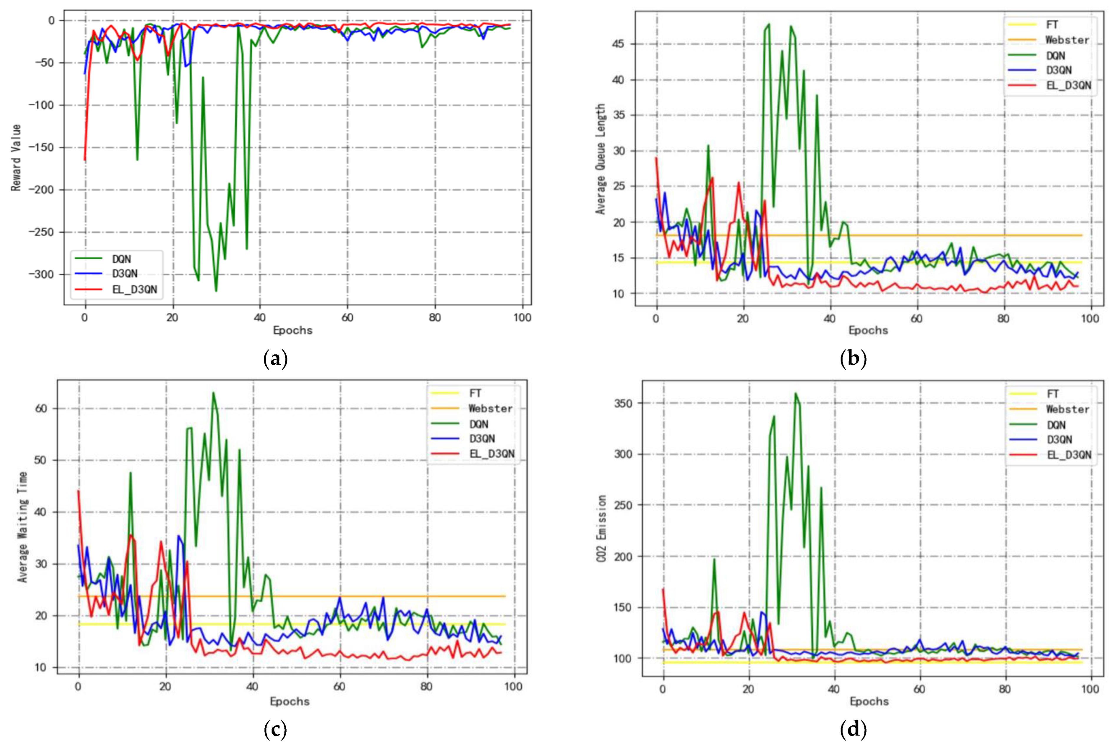
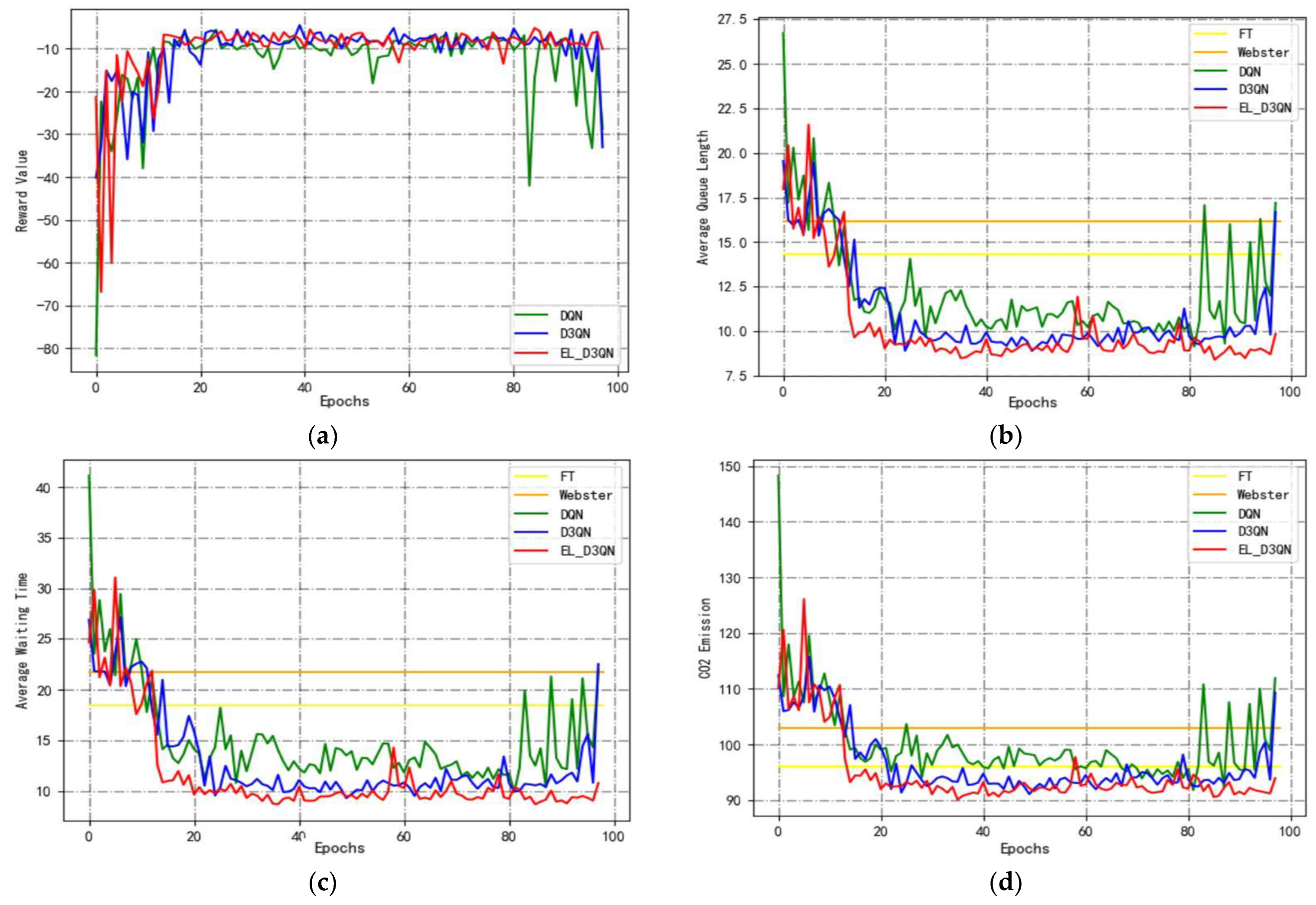
Experiment 1 was conducted based on Configuration 1, and Figure 9 shows a graph comparing the performance of different models in Configuration 1 during training. Figure 9a displays the cumulative reward trend for several models. In the early phase, it continuously increases, and in the later time, it maintains a specific level line. DQN begins to converge at 30 epochs, as can be observed, but the subsequent leaps are substantial because the ideal timing approach has not been identified. D3QN starts to converge at 25 epochs, and its jumps are smaller than that of DQN, but the jumps suddenly become larger after 90 epochs. The EL_D3QN presented in this study begins to converge at 18 epochs and becomes more stable and converge to a particular level. It can also be seen from the result plots of the three evaluation metrics in Figure 9b–d that all three metrics of EL_D3QN are smaller than the other four models, indicating that the performance is better than that of FT, Webster, DQN, and D3QN.

Table 4. Different model performance results for Configuration 1 (train).

Method	Reward	AQL (m)	AWT (s)	CO2 Emissions (g)
FT (30 s)	/	14.290 ↓36.8%	18.464 ↓48.3%	95.999 ↓3.9%
Webster	/	16.151 ↓44.1%	21.754 ↓56.1%	102.942 ↓10.4%
DQN	−15.132 ↑45.7%	12.136 ↓25.6%	14.583 ↓34.6%	99.422 ↓7.2%
D3QN	−9.748 ↑15.7%	10.399 ↓13.2%	11.947 ↓20.2%	95.295 ↓3.2%
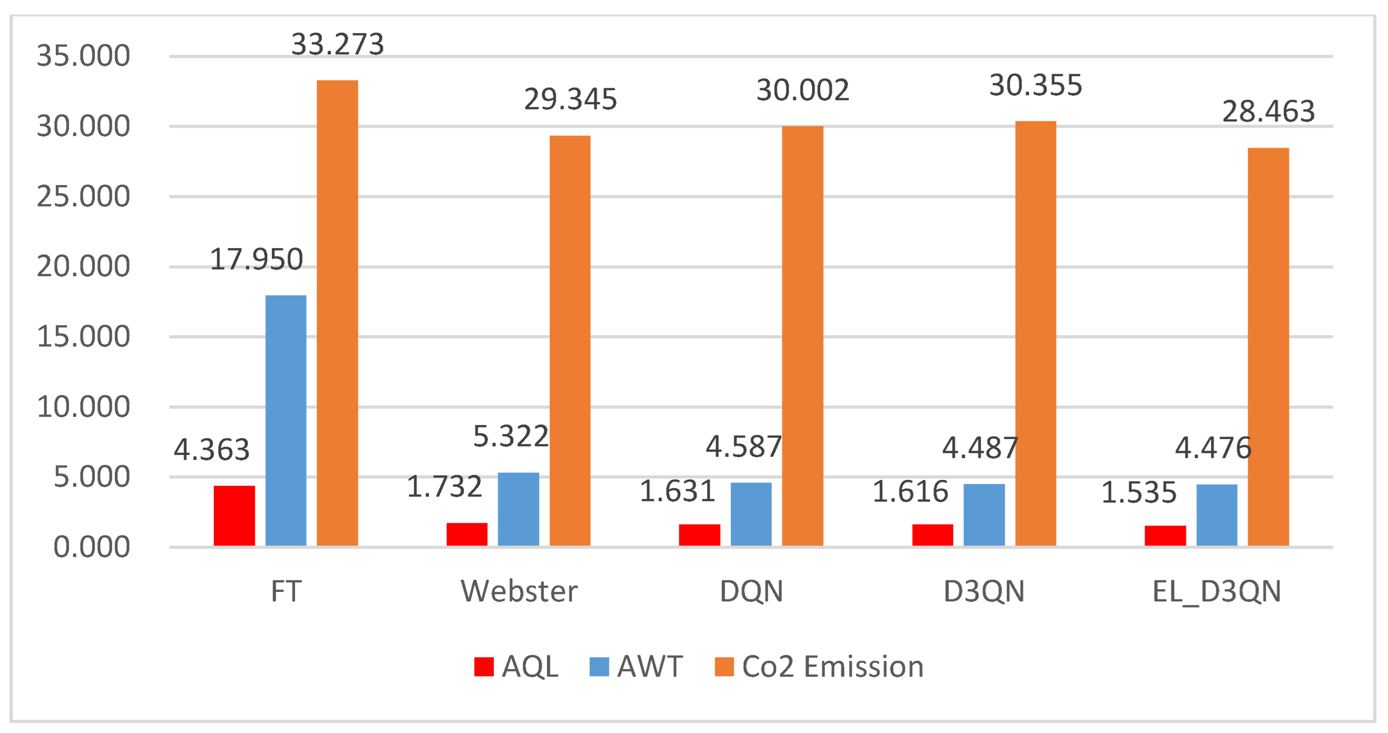
EL_D3QN	−8.220	9.025	9.538	92.229

displays the performance outcomes of different models during Configuration 1 training. The table also shows that the AQL, AWT, and ${\mathrm{C}\mathrm{O}}_2$ emissions of EL_D3QN all decrease when compared to FT by 36.8%, 48.3%, and 3.9%, respectively. The three metrics of EL_D3QN are each decreased by 44.1%, 56.1%, and 10.4% when compared to Webster. This demonstrates how the deep reinforcement learning method can increase the effectiveness of signal control. The cumulative reward of EL_D3QN is 45.7% higher than DQN, and the other three assessment metrics are decreased by 25.6%, 34.6%, and 7.2%, respectively. The AQL, AWT, and ${\mathrm{C}\mathrm{O}}_2$ emissions from this paper are all decreased by 13.2%, 20.2%, and 3.2%, respectively, when compared to D3QN, while the cumulative reward is increased by 15.7%. The data findings and trend graphs from Experiment 1 demonstrate that the control performance of EL_D3QN is more efficient and can lessen the phenomena of traffic congestion.

Figure 9. Performance comparison of different models for Configuration 1 (train). (a) Cumulative reward; (b) average queue length; (c) average waiting time; (d) ${\mathrm{C}\mathrm{O}}_2$ emissions.

Figure 9. Performance comparison of different models for Configuration 1 (train). (a) Cumulative reward; (b) average queue length; (c) average waiting time; (d) ${\mathrm{C}\mathrm{O}}_2$ emissions.

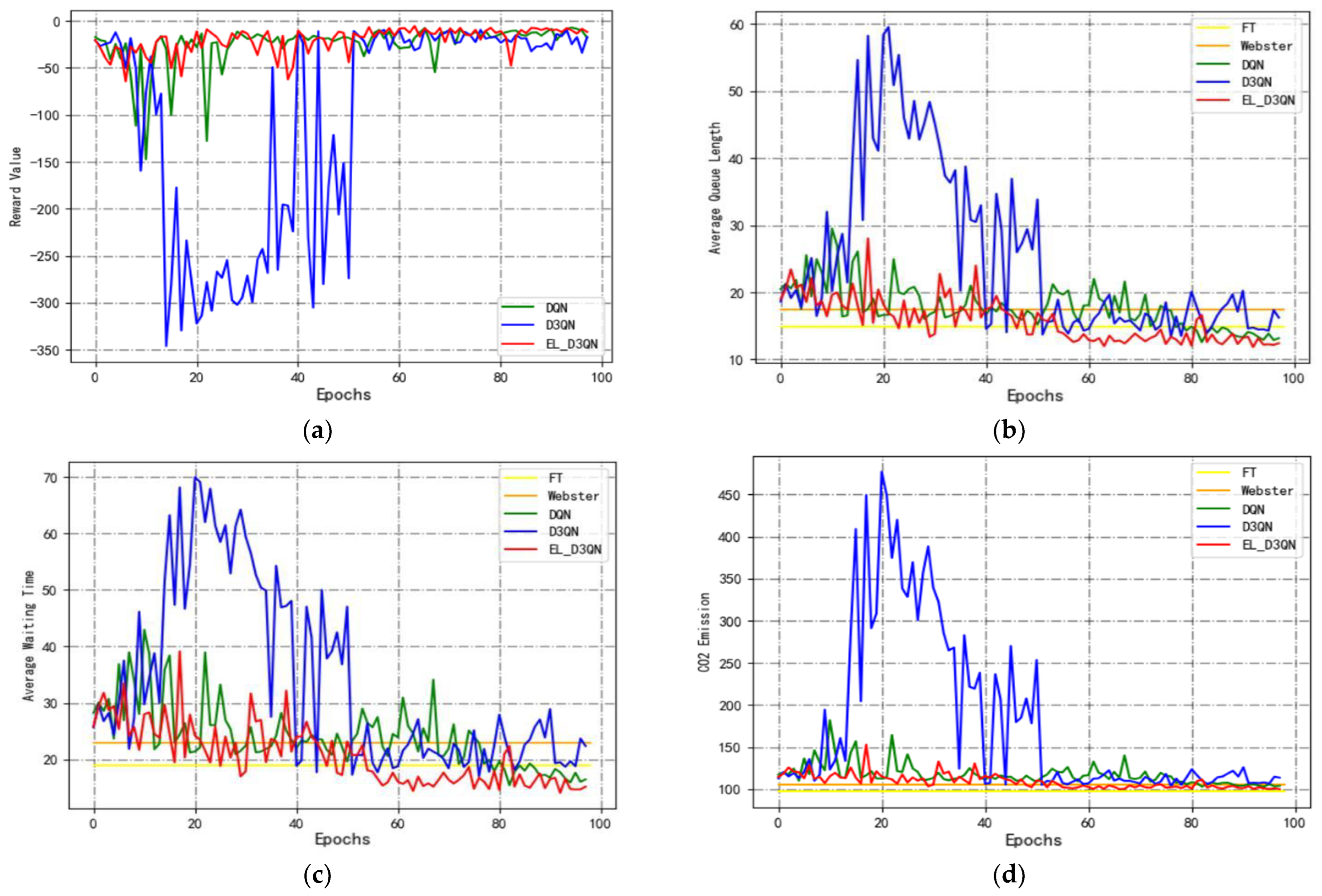
Based on Configuration 2, Experiment 2 is carried out, and the experimental outcomes from the training period are displayed in Figure 10 and Table 5. It is evident from Figure 10a that EL_D3QN has superior convergence and stability than DQN and D3QN. Additionally, EL_D3QN has greater control performance and is more suited to the current setup environment, as shown in Figure 10b–d.

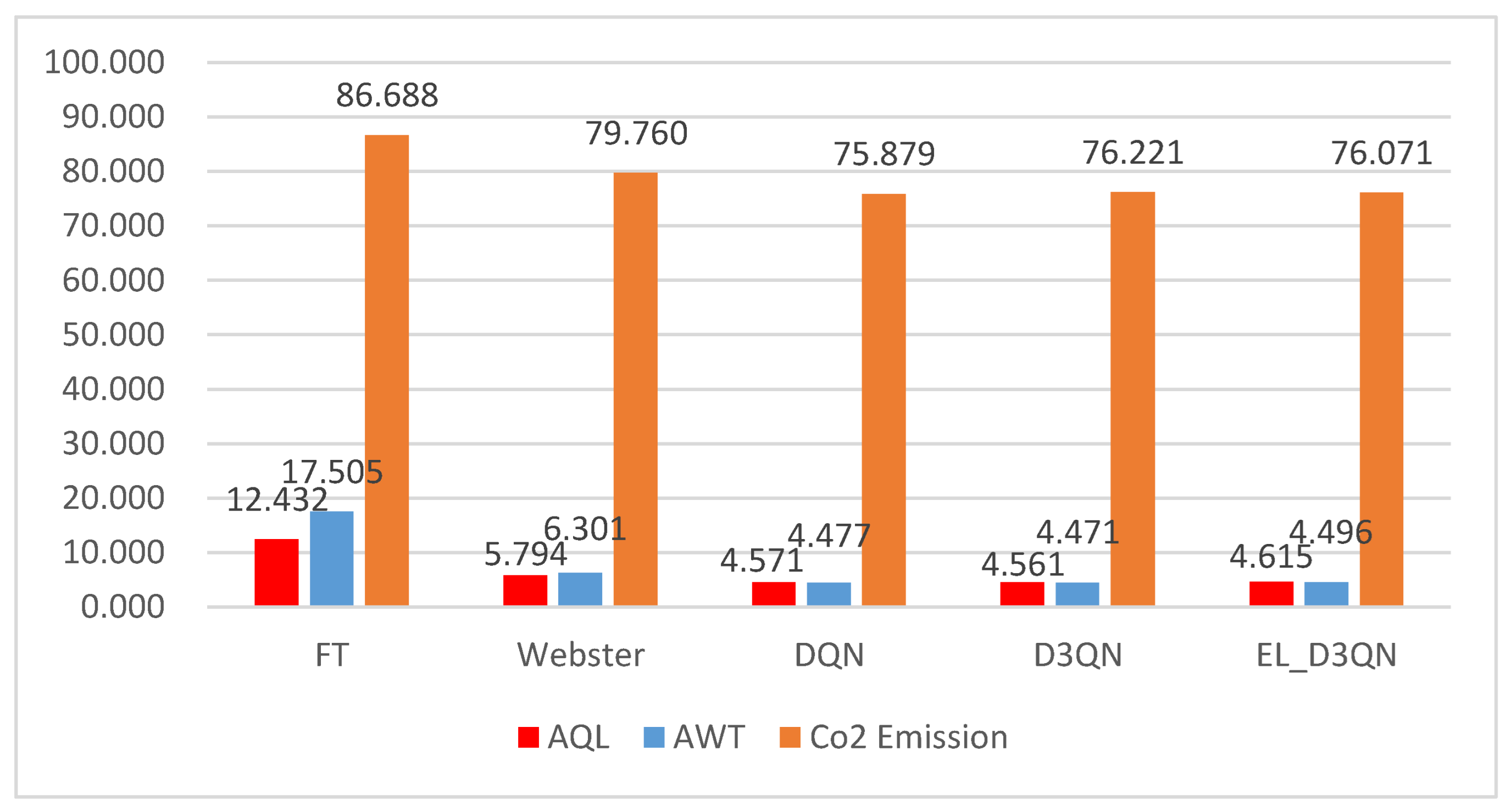
Table 5 shows that, specifically, the AQL and AWT of EL_D3QN decreased by 19.1% and 23.9%, respectively, while the ${\mathrm{C}\mathrm{O}}_2$ emissions increased by 3.4% compared to FT. This was likely due to the smoother vehicle operation in the static condition and the high volatility of the vehicle operation in the dynamic condition, which would result in more serious pollution. For the three metrics, EL_D3QN demonstrated a reduction of 46.4%, 51.5%, and 14.2% in comparison to Webster. The cumulative rewards were increased by 27.7% over DQN, whereas the other three assessment measures were decreased by 10.5%, 14.8%, and 2.6%, respectively. Comparing EL_D3QN to D3QN, the cumulative reward increases by 8.4%, and the AQL, AWT, and ${\mathrm{C}\mathrm{O}}_2$ emissions decrease by 3.0%, 3.2%, and 0.6%, respectively. The data from Experiment 2’s trend graphs and data findings show that EL_D3QN’s control performance is quite successful in this flow scenario.

Figure 10. Performance comparison of different models for Configuration 2 (train). (a) Cumulative reward; (b) average queue length; (c) average waiting time; (d) ${\mathrm{C}\mathrm{O}}_2$ emissions.

Figure 10. Performance comparison of different models for Configuration 2 (train). (a) Cumulative reward; (b) average queue length; (c) average waiting time; (d) ${\mathrm{C}\mathrm{O}}_2$ emissions.

Table 5. Different model performance results for Configuration 2 (train).

Method	Reward	AQL (m)	AWT (s)	CO2 Emissions (g)
FT (30 s)	/	14.757 ↓19.1%	18.888 ↓23.9%	97.098 ↑3.4%
Webster	/	22.283 ↓46.4%	29.598 ↓51.5%	117.088 ↓14.2%
DQN	−10.458 ↑27.7%	13.343 ↓10.5%	16.855 ↓14.8%	103.088 ↓2.6%
D3QN	−8.255 ↑8.4%	12.308 ↓3.0%	14.842 ↓3.2%	101.040 ↓0.6%
EL_D3QN	−7.560	11.945	14.369	100.443

Table 5. Different model performance results for Configuration 2 (train).

Method	Reward	AQL (m)	AWT (s)	CO2 Emissions (g)
FT (30 s)	/	14.757 ↓19.1%	18.888 ↓23.9%	97.098 ↑3.4%
Webster	/	22.283 ↓46.4%	29.598 ↓51.5%	117.088 ↓14.2%
DQN	−10.458 ↑27.7%	13.343 ↓10.5%	16.855 ↓14.8%	103.088 ↓2.6%
D3QN	−8.255 ↑8.4%	12.308 ↓3.0%	14.842 ↓3.2%	101.040 ↓0.6%
EL_D3QN	−7.560	11.945	14.369	100.443

Experiment 3 is carried out in Configuration 3’s traffic environment, and the training period’s experimental outcomes are displayed in Figure 11 and

Table 6. Different model performance results for Configuration 3 (train).

Method	Reward	AQL (m)	AWT (s)	CO2 Emissions (g)
FT (30 s)	/	14.290 ↓22.5%	18.281 ↓29.8%	95.796 ↑3.7%
Webster	/	18.077 ↓38.7%	23.681 ↓45.8%	108.206 ↓8.2%
DQN	−12.931 ↑55.9%	13.882 ↓20.2%	17.440 ↓26.4%	105.426 ↓5.7%
D3QN	−9.515 ↑40.0%	13.037 ↓15.0%	16.545 ↓22.4%	104.598 ↓5.0%
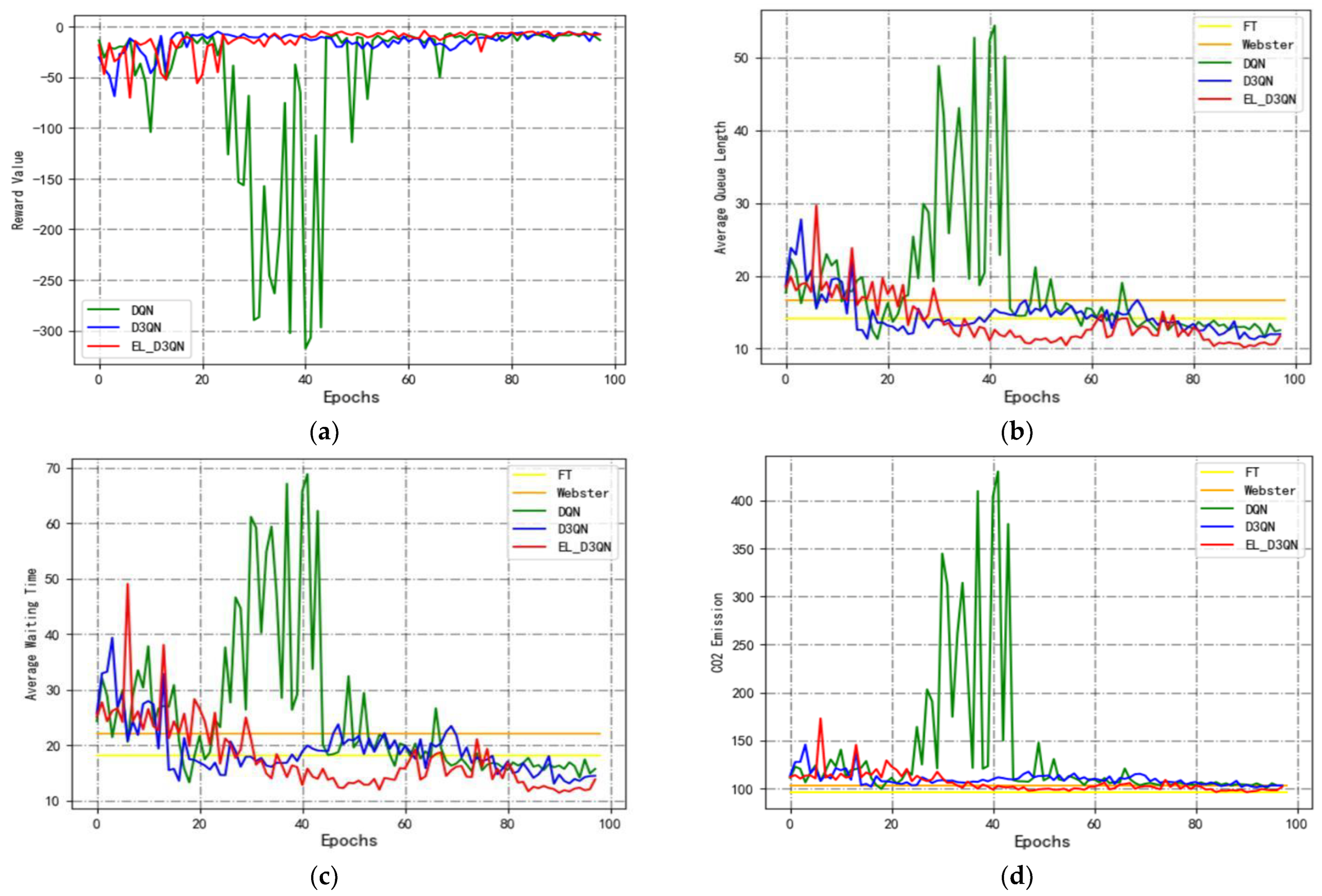
EL_D3QN	−5.705	11.077	12.841	99.384

. Its analytic procedure is identical to Experiment 2’s. From Figure 11, it is clear that EL_D3QN has better stability and convergence than DQN and D3QN, as well as better stability and smoothness than EL_D3QN in Experiment 2. This further suggests that the model in this paper can produce better control results during equal steady peak periods. The control performance of EL_D3QN outperforms the other four approaches, as demonstrated in Table 6.

Figure 11. Performance comparison of different models for Configuration 3 (train). (a) Cumulative reward; (b) average queue length; (c) average waiting time; (d) ${\mathrm{C}\mathrm{O}}_2$ emissions.

Figure 11. Performance comparison of different models for Configuration 3 (train). (a) Cumulative reward; (b) average queue length; (c) average waiting time; (d) ${\mathrm{C}\mathrm{O}}_2$ emissions.

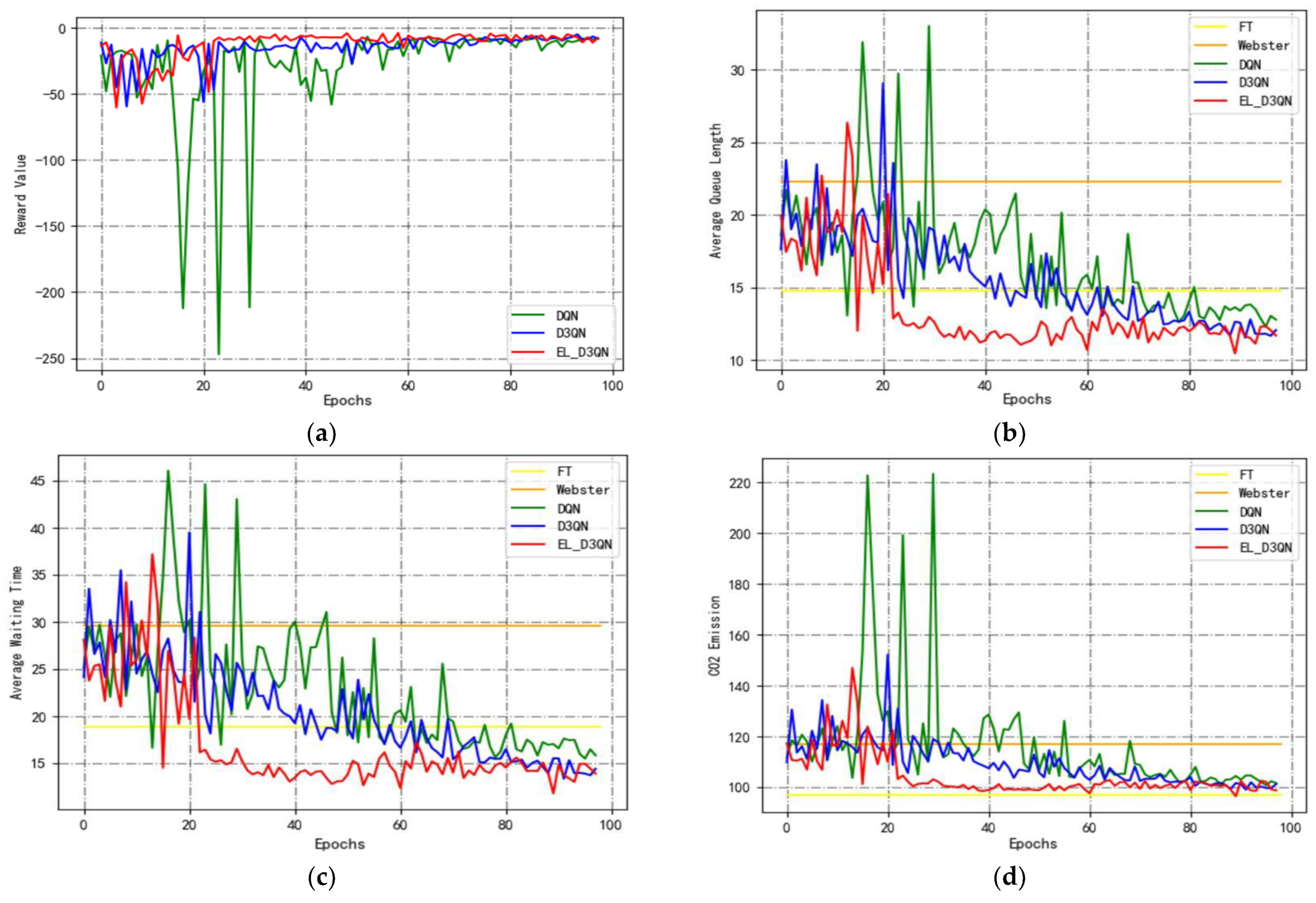
Experiment 4 was carried out in Configuration 4’s traffic environment, and the training period’s experimental outcomes are displayed in Figure 12 and

Table 7. Different model performance results for Configuration 4 (train).

Method	Reward	AQL (m)	AWT (s)	CO2 Emissions (g)
FT (30 s)	/	14.848 ↓11.9%	18.890 ↓13.9%	97.169 ↑5.8%
Webster	/	17.462 ↓25.0%	22.936 ↓29.1%	105.289 ↓2.4%
DQN	−12.945 ↑3.3%	13.903 ↓5.9%	17.669 ↓8.0%	105.85 ↓2.9%
D3QN	−21.345 ↑41.3%	16.438 ↓20.4%	22.234 ↓26.9%	113.117 ↓9.1%
EL_D3QN	−12.522	13.088	16.260	102.774

. The early era of D3QN is evidently quite jumpy from Figure 12a. It takes a long time for the timing scheme to attain convergence since the traffic has a low peak and is unstable. It is stable but has a big jump in the late period. In comparison to D3QN, DQN is more suited to unstable low peak circumstances. Although it also tends to a specific degree of state in the late period, the EL_D3QN jumps are a little bit greater than the jumps from Configuration 1 to Configuration 3, and the control effect is not as strong as that in the first three datasets. Table 7 depicts the overall performance effect and demonstrates that, when compared to other approaches, EL_D3QN has the biggest cumulative reward and the least AQL, AWT, and ${\mathrm{C}\mathrm{O}}_2$ emissions. The outcomes demonstrate that EL_D3QN can significantly enhance control performance.

Figure 12. Performance comparison of different models for Configuration 4 (train). (a) Cumulative reward; (b) average queue length; (c) average waiting time; (d) ${\mathrm{C}\mathrm{O}}_2$ emissions.

Figure 12. Performance comparison of different models for Configuration 4 (train). (a) Cumulative reward; (b) average queue length; (c) average waiting time; (d) ${\mathrm{C}\mathrm{O}}_2$ emissions.

The outcomes of Experiment 5 are displayed in Figure 13 and

Table 8. Different model performance results for Configuration 5 (train).

Method	Reward	AQL (m)	AWT (s)	CO2 Emissions (g)
FT (30 s)	/	14.195 ↓21.9%	18.202 ↓28.9%	95.680 ↑3.4%
Webster	/	16.665 ↓33.5%	22.015 ↓41.2%	103.496 ↓4.4%
DQN	−9.287 ↑28.0%	12.985 ↓14.6%	16.186 ↓20.0%	104.176 ↓5.0%
D3QN	−8.099 ↑17.4%	12.284 ↓9.8%	14.883 ↓13.0%	103.878 ↓4.7%
EL_D3QN	−6.687	11.084	12.948	98.947

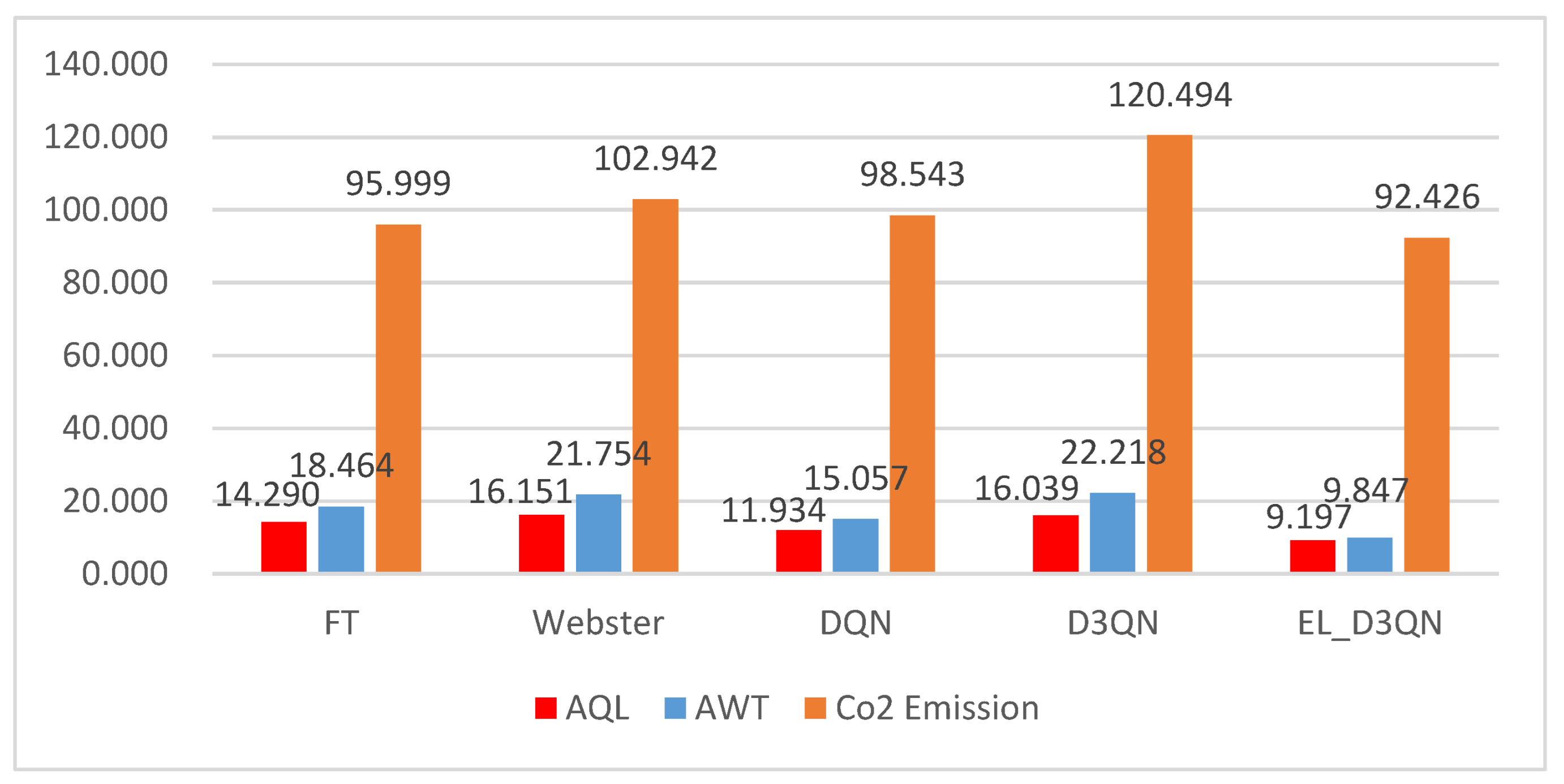
and were carried out in the Configuration 5 traffic scenario. In contrast to the outcomes of Experiment 4, it is evident from Figure 13a that DQN is extremely jumpy upfront. While DQN is more appropriate for instances with unstable low-peak periods, D3QN is more appropriate for those with unstable peak periods. Both cases show that neither of the models performs controls as well as EL_D3QN. Table 8 demonstrates that, in comparison to FT, EL_D3QN decreases the AQL and AWT by 21.9% and 28.9%, respectively, while improving the ${\mathrm{C}\mathrm{O}}_2$ emissions by 3.4%, resulting in an increase in the release that is consistent with Experiments 2, 3, and 4. All three EL_D3QN indices reduced when compared to Webster, DQN, and D3QN. The control performance and stability of EL_D3QN are less stable and perform poorly during the peak time than during the low-peak period, according to a comparison between Experiments 4 and 5.

Figure 13. Performance comparison of different models for Configuration 5 (train). (a) Cumulative reward; (b) average queue length; (c) average waiting time; (d) ${\mathrm{C}\mathrm{O}}_2$ emissions.

Figure 13. Performance comparison of different models for Configuration 5 (train). (a) Cumulative reward; (b) average queue length; (c) average waiting time; (d) ${\mathrm{C}\mathrm{O}}_2$ emissions.

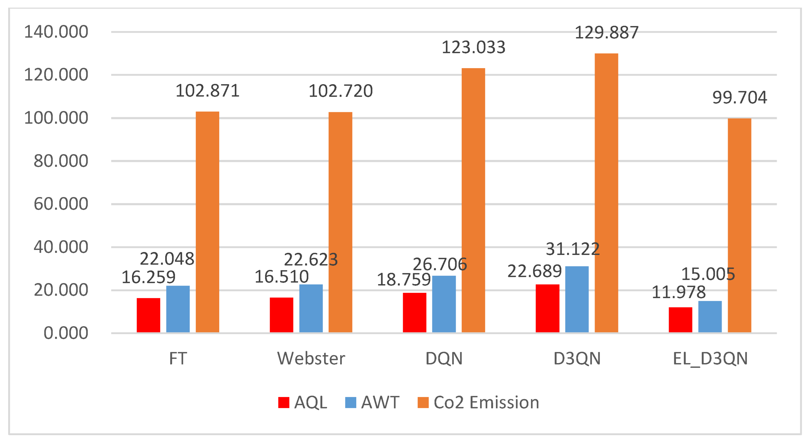
Experiment 6 was tested on a real dataset during a low-peak period, with data for a particular hour on a particular day in Hangzhou, and 19 epochs were tested. It is evident from Figure 14 and

Table 9. Performance results of different algorithms during low peak periods (test).

Method	AQL (m)	AWT (s)	CO2 Emissions (g)
FT (30 s)	4.363 ↓64.8%	17.95 ↓75.1%	33.273 ↓14.5%
Webster	1.732 ↓11.4%	5.322 ↓15.9%	29.345 ↓3.0%
DQN	1.631 ↓5.9%	4.587 ↓2.4%	30.002 ↓5.1%
D3QN	1.616 ↓5.0%	4.487 ↓0.2%	30.355 ↓6.2%
EL_D3QN	1.535	4.476	28.463

that EL_D3QN has lower AQL, AWT, and ${\mathrm{C}\mathrm{O}}_2$ emissions when compared to FT by 64.8%, 75.1%, and 14.5%, respectively. The three measures decreased by 11.4%, 15.9%, and 3.0%, respectively, when compared to Webster. EL_D3QN has the least AQL, AWT, and ${\mathrm{C}\mathrm{O}}_2$ emissions when compared to DQN and D3QN. EL_D3QN performs better under control overall.

A real dataset from the peak time was used to evaluate Experiment 7, with all other variables being the same. The adaptive traffic signal control model outperforms FT and Webster, as demonstrated in Figure 15 and

Table 10. Performance results of different algorithms during peak periods (test).

Method	AQL (m)	AWT (s)	CO2 Emission (g)
FT (30 s)	12.432 ↓62.9%	17.505 ↓74.3%	86.688 ↓12.2%
Webster	5.794 ↓20.3%	6.301 ↓28.6%	79.760 ↓4.6%
DQN	4.571 ↑1.0%	4.477 ↑0.4%	75.879 ↑0.3%
D3QN	4.561 ↑1.2%	4.471 ↑0.6%	76.221 ↓0.2%
EL_D3QN	4.615	4.496	76.071

. All three adaptive approaches can reduce traffic congestion during peak hours; however, EL_D3QN performs somewhat worse in terms of control than the other two.

The results of several sets of experiments using the simulation experiments with various traffic configurations demonstrated that EL_D3QN has good control performance and its ability to generalize, with the exception of Experiment 7, where its performance is marginally inferior to that of the other two control methods, but the control effect is still good.

5.3.3. Special Scenario Test Research

This section of the article opts to build on Configuration 1’s synthetic dataset and sets up two unique situations to test. Each scenario is tested for a total of 19 epochs.

Experiment 1 involves a traffic surge scenario in which there is a significant sporting event in the west. As a result, the arrival rates of vehicles in the east–west straight direction, north–west right turn, and south–west left turn directions, which are 0.5, 0.3, and 0.3, respectively, all suddenly increase in the second half of the hour. As can be shown from Figure 16 and

Table 11. Different model performance results for Scenario 1 (test).

Method	AQL (m)	AWT (s)	CO2 Emissions (g)
FT (30 s)	14.290 ↓35.6%	18.464 ↓46.7%	95.999 ↑3.7%
Webster	16.151 ↓43.1%	21.754 ↓54.7%	102.942 ↓10.2%
DQN	11.934 ↓22.9%	15.057 ↓34.6%	98.543 ↓6.2%
D3QN	16.039 ↓42.7%	22.218 ↓55.7%	120.494 ↓23.3%
EL_D3QN	9.197	9.847	92.426

, the EL_D3QN’s AQL and AWT decrease by 35.6% and 46.7%, respectively, in comparison to the FT, and the ${\mathrm{C}\mathrm{O}}_2$ emissions increase by 3.7%. Compared to Webster, DQN, and D3QN, it emits the least AQL, AWT, and ${\mathrm{C}\mathrm{O}}_2$ emissions.

In Experiment 2, a road capacity limitation situation is simulated, wherein some road sections have traffic accidents or are unable to undergo construction. The south entrance left turn lane serves as the construction road in this article. Figure 17 and

Table 12. Different model performance results for Scenario 2 (test).

Method	AQL (m)	AWT (s)	CO2 Emissions (g)
FT (30 s)	16.259 ↓26.3%	22.048 ↓31.9%	102.871 ↑3.1%
Webster	16.510 ↓27.4%	22.623 ↓33.7%	102.720 ↓2.9%
DQN	18.759 ↓36.1%	126.706 ↓43.8%	123.033 ↓19.0%
D3QN	22.689 ↓47.2%	31.122 ↓51.8%	129.887 ↓23.2%
EL_D3QN	11.978	15.005	99.704

illustrate how EL_D3QN improves ${\mathrm{C}\mathrm{O}}_2$ emissions by 3.1% while reducing AQL and AWT by 26.3% and 31.9%, respectively, when compared to FT. In comparison to the other three approaches, EL_D3QN has the lowest three metrics.

Overall, the other four models are weakly resilient and unable to handle unique scenarios. Good control performance and robustness allow EL_D3QN to perform normally in unusual circumstances.

6. Conclusions

This research proposes an improved D3QN algorithm-based EL_D3QN control framework for signal timing. The D3QN network structure is altered by adding ECA and LSTM modules. The input consists of vehicle position and speed data gathered by the camera, and the reward is the total waiting time difference between two moments. In this work, ablation experiments, various vehicle conditions, and unique scenario experiments are used to confirm the viability and control performance of the model. The results demonstrate that EL_D3QN performs better than the other four models in the presence of unequal stability, equal stability, or complex traffic scenarios. It has good control performance and generalization ability and can successfully resolve the traffic congestion problem in a variety of road conditions. When special circumstances such as traffic surges occur, EL_D3QN can still achieve good control effect and robustness. However, its high complexity may affect the response time.

In future work, we will conduct further research on how to reduce the response time. In addition, this paper only conducted experimental verification for a single intersection, and the adaptive traffic signal control system for multiple intersections can be studied in the future. With the increase in the number of intersections, how to coordinate multiple intersections for effective signal timing control under simple state information can be studied. The reward definition of a single intersection is not necessarily adapted to multiple intersections, and it is also necessary to explore the reward space of multiple intersections. In addition, the pedestrian factor can also be considered in the problems solved in this paper.

References

1. Guzmán, J.A.; Pizarro, G.; Núñez, F. A reinforcement learning-based distributed control scheme for cooperative intersection traffic control. IEEE Access 2023, 11, 57037–57045. [Google Scholar] [CrossRef]
2. Mikkonen, S.; Laine, M.; Mäkelä, H.M.; Gregow, H.; Tuomenvirta, H.; Lahtinen, M.; Laaksonen, A. Trends in the average temperature in Finland, 1847–2013. Stoch. Environ. Res. Risk Assess. 2015, 29, 1521–1529. [Google Scholar] [CrossRef]
3. Gokasar, I.; Timurogullari, A.; Deveci, M.; Garg, H. SWSCAV: Real-time traffic management using connected autonomous vehicles. ISA Trans. 2023, 132, 24–38. [Google Scholar] [CrossRef] [PubMed]
4. Noaeen, M.; Naik, A.; Goodman, L.; Crebo, J.; Abrar, T.; Abad, Z.S.H.; Bazzan, A.L.C.; Far, B. Reinforcement learning in urban network traffic signal control: A systematic literature review. Expert Syst. Appl. 2022, 199, 116830. [Google Scholar] [CrossRef]
5. Miletić, M.; Ivanjko, E.; Gregurić, M.; Krešimir, K. A review of reinforcement learning applications in adaptive traffic signal control. IET Intell. Transp. Syst. 2022, 16, 1269–1285. [Google Scholar] [CrossRef]
6. Mannion, P.; Duggan, J.; Howley, E. An experimental review of reinforcement learning algorithms for adaptive traffic signal control. In Autonomic Road Transport Support Systems; Birkhäuser: Cham, Switzerland, 2016; pp. 47–66. [Google Scholar] [CrossRef]
7. Shakya, A.K.; Pillai, G.; Chakrabarty, S. Reinforcement Learning Algorithms: A brief survey. Expert Syst. Appl. 2023, 231, 120495. [Google Scholar] [CrossRef]
8. Balaji, P.G.; German, X.; Srinivasan, D. Urban traffic signal control using reinforcement learning agents. IET Intell. Transp. Syst. 2010, 4, 177–188. [Google Scholar] [CrossRef]
9. Zhang, H.; Liu, C.; Zhang, W.; Zheng, G.; Yu, Y. Generalight: Improving environment generalization of traffic signal control via meta reinforcement learning. In Proceedings of the 29th ACM International Conference on Information & Knowledge Management, Chengdu, China, 19–23 October 2020; pp. 1783–1792. [Google Scholar]
10. Watkins, C.J.C.H.; Dayan, P. Q-learning. Mach. Learn. 1992, 8, 279–292. [Google Scholar] [CrossRef]
11. Matsuo, Y.; LeCun, Y.; Sahani, M.; Precup, D.; Silver, D.; Sugiyama, M.; Uchibe, E.; Morimoto, J. Deep learning, reinforcement learning, and world models. Neural Netw. 2022, 152, 267–275. [Google Scholar] [CrossRef]
12. Gregurić, M.; Vujić, M.; Alexopoulos, C.; Miletić, M. Application of deep reinforcement learning in traffic signal control: An overview and impact of open traffic data. Appl. Sci. 2020, 10, 4011. [Google Scholar] [CrossRef]
13. Haydari, A.; Yılmaz, Y. Deep reinforcement learning for intelligent transportation systems: A survey. IEEE Trans. Intell. Transp. Syst. 2020, 23, 11–32. [Google Scholar] [CrossRef]
14. Liao, L.; Liu, J.; Wu, X.; Zou, F.; Pan, J.; Sun, Q.; Li, S.E.; Zhang, M. Time difference penalized traffic signal timing by LSTM Q-network to balance safety and capacity at intersections. IEEE Access 2020, 8, 80086–80096. [Google Scholar] [CrossRef]
15. Liu, J.; Qin, S.; Luo, Y.; Wang, Y.; Yang, S. Intelligent traffic light control by exploring strategies in an optimised space of deep Q-learning. IEEE Trans. Veh. Technol. 2022, 71, 5960–5970. [Google Scholar] [CrossRef]
16. Zhang, R.; Ishikawa, A.; Wang, W.; Striner, B.; Tongux, Q.K. Using reinforcement learning with partial vehicle detection for intelligent traffic signal control. IEEE Trans. Intell. Transp. Syst. 2020, 22, 404–415. [Google Scholar] [CrossRef]
17. Ibrokhimov, B.; Kim, Y.J.; Kang, S. Biased pressure: Cyclic reinforcement learning model for intelligent traffic signal control. Sensors 2022, 22, 2818. [Google Scholar] [CrossRef] [PubMed]
18. Zhao, X.; Flocco, D.; Azarm, S.; Balavhandran, B. Deep Reinforcement Learning for the Co-Optimization of Vehicular Flow Direction Design and Signal Control Policy for a Road Network. IEEE Access 2023, 11, 7242–7261. [Google Scholar] [CrossRef]
19. Liang, X.; Du, X.; Wang, G.; Han, Z. A deep reinforcement learning network for traffic light cycle control. IEEE Trans. Veh. Technol. 2019, 68, 1243–1253. [Google Scholar] [CrossRef]
20. Liu, Z.; Cao, S.; Shen, Y.; Yang, X. Signal Control of Single Intersection Based on Improved Deep Reinforcement Learning Method. Comput. Sci. 2020, 47, 226–232. [Google Scholar]
21. Wang, B.; He, Z.; Sheng, J.; Chen, Y. Deep Reinforcement Learning for Traffic Light Timing Optimization. Processes 2022, 10, 2458. [Google Scholar] [CrossRef]
22. Savithramma, R.M.; Sumathi, R.; Sudhira, H.S. Reinforcement learning based traffic signal controller with state reduction. J. Eng. Res. 2023, 11, 100017. [Google Scholar] [CrossRef]
23. Lu, L.; Cheng, K.; Chu, D.; Wu, C.; Qiu, Y. Adaptive traffic signal control based on dueling recurrent double Q network. China J. Highw. Transp. 2022, 35, 267–277. [Google Scholar]
24. Wang, H.; Zhu, J.; Gu, B. Model-Based Deep Reinforcement Learning with Traffic Inference for Traffic Signal Control. Appl. Sci. 2023, 13, 4010. [Google Scholar] [CrossRef]
25. Han, G.; Zheng, Q.; Liao, L.; Tang, P.; Li, Z.; Zhu, Y. Deep reinforcement learning for intersection signal control considering pedestrian behavior. Electronics 2022, 11, 3519. [Google Scholar] [CrossRef]
26. Kolat, M.; Kővári, B.; Bécsi, T.; Aradi, S. Multi-agent reinforcement learning for traffic signal control: A cooperative approach. Sustainability 2023, 15, 3479. [Google Scholar] [CrossRef]
27. Zaman, S.K.U.; Jehangiri, A.I.; Maqsood, T.; Umar, A.I.; Khan, M.A.; Jhanjhi, N.Z.; Shorfuzzaman, M.; Masud, M. COME-UP: Computation offloading in mobile edge computing with LSTM based user direction prediction. Appl. Sci. 2022, 12, 3312. [Google Scholar] [CrossRef]
28. Xu, D.; Li, C.; Wang, D.; Gao, G. Robustness Analysis of Discrete State-Based Reinforcement Learning Models in Traffic Signal Control. IEEE Trans. Intell. Transp. Syst. 2022, 24, 1727–1738. [Google Scholar] [CrossRef]
29. Zhang, Z.; Guo, M.; Fu, D.; Mo, L.; Zhang, S. Traffic signal optimization for partially observable traffic system and low penetration rate of connected vehicles. Comput.-Aided Civ. Infrastruct. Eng. 2022, 37, 2070–2092. [Google Scholar] [CrossRef]
30. Zhao, T.; Wang, P.; Li, S. Traffic signal control with deep reinforcement learning. In Proceedings of the 2019 International Conference on Intelligent Computing, Automation and Systems (ICICAS), Chongqing, China, 6–8 December 2019; pp. 763–767. [Google Scholar]
31. Xu, M.; Wu, J.; Huang, L.; Zhou, R.; Wang, T.; Hu, D. Network-wide traffic signal control based on the discovery of critical nodes and deep reinforcement learning. J. Intell. Transp. Syst. 2020, 24, 1–10. [Google Scholar] [CrossRef]
32. Wu, T.; Zhou, P.; Liu, K.; Yuan, Y.; Wang, X.; Huang, H.; Wu, D.O. Multi-agent deep reinforcement learning for urban traffic light control in vehicular networks. IEEE Trans. Veh. Technol. 2020, 69, 8243–8256. [Google Scholar] [CrossRef]
33. Wang, Q.; Wu, B.; Zhu, P.; Li, P.; Zuo, W.; Hu, Q. ECA-Net: Efficient channel attention for deep convolutional neural networks. In Proceedings of the IEEE/CVF Conference on Computer Vision and Pattern Recognition, Seattle, WA, USA, 16–20 June 2020; pp. 11534–11542. [Google Scholar]
34. Pranolo, A.; Mao, Y.; Wibawa, A.P.; Utama, A.B.P.; Dwiyanto, F.A. Robust LSTM With tuned-PSO and bifold-attention mechanism for analyzing multivariate time-series. IEEE Access 2022, 10, 78423–78434. [Google Scholar] [CrossRef]
35. Li, L.; Wen, D. Parallel systems for traffic control: A rethinking. IEEE Trans. Intell. Transp. Syst. 2015, 17, 1179–1182. [Google Scholar] [CrossRef]
36. Genders, W.; Razavi, S. Using a deep reinforcement learning agent for traffic signal control. arXiv 2016, arXiv:1611.01142. [Google Scholar]
37. Kumar, N.; Rahman, S.S.; Dhakad, N. Fuzzy inference enabled deep reinforcement learning-based traffic light control for intelligent transportation system. IEEE Trans. Intell. Transp. Syst. 2020, 22, 4919–4928. [Google Scholar] [CrossRef]
Figure 1. Traffic signal control model.
Sustainability 15 13668 g001
Figure 2. (a) Single intersection model; (b) the phase sequence diagram.
Sustainability 15 13668 g002
Figure 3. Road state space design diagram.
Sustainability 15 13668 g003
Figure 4. Structure of the improved neural network.
Sustainability 15 13668 g004
Figure 5. ECA-NET structure.
Sustainability 15 13668 g005
Figure 6. LSTM architecture.
Sustainability 15 13668 g006
Figure 7. System framework.
Sustainability 15 13668 g007
Figure 8. Comparison of ablation experiments. (a) Cumulative reward; (b) average queue length; (c) average waiting time; (d) C O 2 emissions.
Sustainability 15 13668 g008
Figure 14. Performance comparison of different algorithms during low peak periods (test).
Sustainability 15 13668 g014
Figure 15. Performance comparison of different algorithms during peak periods (test).
Sustainability 15 13668 g015
Figure 16. Performance comparison of different models for Scenario 1 (test).
Sustainability 15 13668 g016
Figure 17. Performance comparison of different models for Scenario 2 (test).
Sustainability 15 13668 g017