State Estimation of Distributed Drive Electric Vehicle Based on Adaptive Kalman Filter

Abstract

As a new type of transportation, the distributed drive electric vehicle is regarded as the main development direction of electric vehicles in the future. Due to the advantages of the independently controllable driving torque of each wheel, it provides more favorable conditions for vehicle active safety control. Acquiring accurate and real-time parameters such as vehicle speed and side slip angle is a prerequisite for vehicle active safety control. Therefore, relying on the National Natural Science Foundation of China, this paper takes the distributed drive electric vehicle in the form of four-wheel independent drive and steering as the research object. Taking the measurement data of low-cost vehicle sensors as input and adaptive Kalman filtering as theoretical support, the sub-filter of federal Kalman filtering adds a fuzzy controller on the basis of volumetric Kalman filtering, and designs the vehicle driving state estimation algorithm to realize the accurate estimation of driving state information. Finally, the typical experimental conditions are selected, and the designed algorithm is verified by the co-simulation of MATLAB/Simulink and CarSim. At the same time, the algorithm is further verified based on the driving simulator hardware-in-the-loop experimental platform. The results show that the designed estimation algorithm has good effects in terms of accuracy, stability, and real-time performance.

1. Introduction

The advantage of distributed drive electric vehicles is that the energy source that provides the power is the battery, which is a stable, efficient, and environmentally non-polluting energy source. On the other hand, due to the unique structure of distributed drive, it is obviously superior to traditional vehicles in terms of stability, active safety, and saving energy. There is no doubt that this drive method has become the mainstream development direction of the new generation of electric vehicles [1,2,3,4,5]. In dynamics control, based on the current state information, the control algorithm analyzes it to decide to execute the corresponding control strategy. Therefore, the accuracy of the provided vehicle state parameters largely determines the performance of the control algorithm [6,7,8,9]. As a crucial link in closed-loop control, the acquisition of state variables plays a decisive role.

Driving state information, such as vehicle speed and center-of-mass side deviation angle, is an important prerequisite for vehicle control. The Kalman filter algorithm is the most common method used to estimate vehicle state parameters. As a numerical estimation optimization method, the Kalman filter mainly includes two parts: prediction and correction [10]. In reference [11], the vehicle model combines kinematics and dynamics to estimate the driving state information of the vehicle, with the extended Kalman filter (EKF) as the theoretical guide. In reference [12], the dynamic model of three degrees of freedom is used as the estimation model, and the nonlinear equation is linearized by the method of Taylor series expansion to realize the estimation of the vehicle state. This method is suitable for nonlinear systems, and the estimation effect is good. Wenzel scholars and others [13] constructed a double EKF, which exchange information between different variables during the estimation process and correct each other continuously, constituting a closed-loop feedback system that reduces the estimation error. Reference [14] introduced fuzzy theory on the basis of EKF theory to realize the estimation of vehicle longitudinal velocity, and the input of the algorithm is wheel speed and wheel acceleration. This method enhances the adaptability of the algorithm by dynamically adjusting the estimated parameters. Reference [15] introduced the genetic algorithm based on the unscented Kalman filter (UKF) theory to complete the high-precision estimation of the driving state of the traditional front-wheel-steered vehicle. Reference [16] proposes an adaptive UKF speed estimation algorithm, which realizes the adaptive adjustment of the covariance between the measurement noise and the process noise during the estimation process. Reference [17] proposed an UKF algorithm. The Huber cost function was introduced to correct the measured noise and state covariance in real time to improve the robustness of the observer. Reference [18] uses the square-root cubature Kalman filter (CKF) with the maximum correlation entropy criterion (MCSRCKF), which has high accuracy and enhanced robustness for distributed drive vehicle state estimation problems in real non-Gaussian noise environments. In reference [19], aiming at the uncertainty of the noise covariance matrix in the UKF process, the ant lion optimization algorithm (ALO) is used to optimize it.

Based on the above research, it can be found that vehicle traveling state estimation can also be combined with research in other fields, such as machine learning and deep learning. By utilizing machine learning and deep learning algorithms, patterns and features can be learned from a large amount of data to improve the accuracy and robustness of vehicle driving state estimation further. However, vehicle driving state estimation requires processing and analyzing a large amount of data to extract useful information. In practice, it is necessary to ensure that the estimation algorithm has low computational complexity and can produce accurate estimation results in a short time. At the same time, distributed drive electric vehicle driving state estimation also needs to consider the characteristics of the power system and real-time requirements. The power system of an electric vehicle is relatively complex, including components such as motor, battery, and control system, which requires real-time acquisition and processing of information from each component. Therefore, it is a challenging problem to establish an accurate simulation model of the whole vehicle to realize high-precision driving state estimation under the premise of meeting the real-time requirements. In addition, how to establish a set of unified assessment indicators and evaluation system to compare the advantages and disadvantages of different methods and to promote the further development of research is also an important research direction.

This paper takes a four-wheel independent drive and four-wheel independent steering distributed drive electric vehicle as a carrier, comprehensively considers the real time and accuracy of the estimation method, and introduces an external motor to establish a vehicle estimation and vehicle simulation model. Based on the theory of FKF, the sub-filter introduces a fuzzy adaptive based on CKF, and the complete design of an algorithm that can be used to estimate the vehicle driving state information accurately, aiming to provide a theoretical basis for the research and development of the new generation of electric vehicles and active safety control. The offline simulation test is carried out using CarSim (v2019.0) and MATLAB/Simulink software (R2021b), and the real-time simulation is applied to the driving simulator test bed.

2. Modeling of Distributed Drive Electric Vehicles

The establishment of the estimation model of the distributed drive electric vehicle is the basis of the driving state estimation algorithm, and the accuracy of the model is closely related to the estimation accuracy of the algorithm.

2.1. Three-Degrees-of-Freedom Vehicle Model

Considering the actual research needs and the real-time performance of the calculation, the vehicle model is simplified and a nonlinear dynamic model is built. The following assumptions are made about the established model:

(1)

The coordinate origin of the vehicle dynamics model coincides with the mass center;

(2)

The body is rigid and the four wheels are controlled independently of each other;

(3)

The characteristics of each tire are the same;

(4)

The influence of the suspension system on the vehicle motion is ignored.

The vehicle dynamics model is shown in Figure 1, where x and y represent the longitudinal and lateral motion, respectively, and the direction of the yaw rate is marked in Figure 1.

The longitudinal and lateral accelerations at the center of mass and the yaw acceleration are expressed as:

$$\mathrm{u}=a_x+vr$$

(1)

$$\stackrel{.}{v}=a_y-ur$$

(2)

$$\stackrel{\cdot }{r}=\frac{1}{I_z}\mathrm{\Gamma }$$

(3)

The equations of vehicle dynamics are as follows:

$$\begin{array}{l}{ma}_x=F_{x\_fl}\cos {\delta }_{fl}-F_{y\_fl}\sin {\delta }_{fl}{+F}_{x\_fr}\cos {\delta }_{fr}-F_{y\_fr}\sin {\delta }_{fr}\\ {\begin{array}{cc}& \end{array} +F}_{x\_rl}\cos {\delta }_{rl}+F_{y\_rl}\sin {\delta }_{rl}+F_{x\_rr}\cos {\delta }_{rr}+F_{y\_rr}\sin {\delta }_{rr}\end{array}$$

(4)

$$\begin{array}{c}{ma}_y=F_{x\_fl}\sin {\delta }_{fl}+F_{y\_fl}\cos {\delta }_{fl}+F_{x\_fr}\sin {\delta }_{fr}+F_{y\_fr}\cos {\delta }_{fr}\hfill \\ { -F}_{x\_rl}\sin {\delta }_{rl}+F_{y\_rl}\cos {\delta }_{rl}-F_{x\_rr}\sin {\delta }_{rr}+F_{y\_rr}\cos {\delta }_{rr}\end{array}$$

(5)

$$\begin{array}{l}\mathrm{\Gamma }=a(F_{x\_fl}\sin {\delta }_{fl}+F_{y\_fl}\cos {\delta }_{fl})-\frac{t_f}{2}(F_{x\_fl}\cos {\delta }_{fl}-F_{y\_fl}\sin {\delta }_{fl})\\ +a(F_{x\_fr}\sin {\delta }_{fr}+F_{y\_fr}\cos {\delta }_{fl})+\frac{t_f}{2}(F_{x\_fr}\cos {\delta }_{fr}-F_{y\_fr}\sin {\delta }_{fr})\\ +b(F_{x\_rl}\cos {\delta }_{rl}-F_{y\_rl}\sin {\delta }_{rl})-\frac{t_r}{2}(F_{x\_rl}\cos {\delta }_{rl}+F_{y\_rl}\sin {\delta }_{rl})\\ +b(F_{x\_rr}\cos {\delta }_{rr}-F_{y\_rr}\sin {\delta }_{rr})+\frac{t_r}{2}(F_{x\_rr}\cos {\delta }_{rr}+F_{y\_rr}\sin {\delta }_{rr})\end{array}$$

(6)

In order to reduce the error caused by the tire model itself to calculate the tire force, the longitudinal force of the tire is obtained by calculating the four-wheel drive torque, as shown in Equation (7).

$$F_{x\_ij}=T_{ij}-\frac{J_{ij}.{\stackrel{.}{\omega }}_{ij}}{R_e}$$

(7)

2.2. Tire Model

The Dugoff tire model is an analytical model derived from the balance of forces, where the longitudinal force and lateral force have a direct relationship with the friction coefficient between the tire and the road surface, and the road surface attachment coefficient can be separated independently, which is conducive to the next step in the design of the estimation algorithm of the road surface attachment coefficient [20,21,22].

In the Dugoff tire model, the lateral force of the tire can be directly calculated by the slip rate [23], and the formula is as follows:

$$F_{y\_ij}={\mu }_{\_ij}{F}_{z\_ij}{C}_y\frac{\tan ({\alpha }_{ij})}{1-{\lambda }_{\_ij}}f\left(L\right), f(L)=\left\{\begin{array}{c}L\cdot (2-L),L<1\\ \begin{array}{ccc}& 1& \end{array} ,L\ge 1\end{array}\right.$$

(8)

where

$$L=\frac{1}{\sqrt[2]{C_x^2{\lambda }_{\_ij}^2+C_y^2{\tan }^2{\alpha }_{\mathrm{ij}}}}(1-{\lambda }_{\_ij})\times (1-\epsilon \cdot u_{\_ij}\cdot \sqrt{C_x^2{\lambda }_{\_ij}^2+C_y^2{\tan }^2{\alpha }_{\mathrm{ij}}})$$

(9)

$${\alpha }_{fl,fr}={\delta }_{fl,fr}-\arctan (\frac{v+ar}{u\pm \frac{t_f}{2}r}), {\alpha }_{rl,rr}={\delta }_{rl,rr}-\arctan (\frac{-v+br}{u\pm \frac{t_r}{2}r})$$

(10)

$$F_{z\_fl,fr}=(\frac{1}{2}mg\pm m{a}_y\frac{h}{t_f})\frac{b}{l}-\frac{1}{2}m{a}_x\frac{h}{l}, F_{z\_rl,rr}=(\frac{1}{2}mg\pm m{a}_y\frac{h}{t_r})\frac{b}{l}+\frac{1}{2}m{a}_x\frac{h}{l}$$

(11)

The value of the slip rate is:

$$\left\{\begin{array}{l}{\lambda }_{ij}=\frac{R_e{\omega }_{ij}-v_{ij}}{v_{ij}}=\frac{R_e{\omega }_{ij}}{v_{ij}}-1<0\begin{array}{c}\end{array}(\mathrm{brake})\\ {\lambda }_{ij}=\frac{R_e{\omega }_{ij}-v_{ij}}{R_e{v}_{ij}}=1-\frac{v_{ij}}{R_e{\omega }_{ij}}>0\begin{array}{c}\end{array}(\mathrm{drive})\end{array}\right.$$

(12)

where

$$v_{fl,fr}=\sqrt{{(u\pm \frac{t_f}{2}r)}^2+{(v+ar)}^2}{,v}_{rl,rr}=\sqrt{{(u\pm \frac{t_r}{2}r)}^2+{(v-br)}^2}$$

(13)

In the above equation, i = $f$ or $r$ represents the front or rear wheel, and $j$ = l or $r$ represents the left or right wheel.

The tire stiffness has a great influence on the accuracy of the model. In the original Dugoff model, the tire stiffness does not change with the change of the vertical load. Since the influence of the load is the largest, this paper only considers this influencing factor and ignores other factors. The tire stiffness is obtained by fitting the test data with the tire model built by CarSim. Figure 2 shows the relationship between tire characteristics under different vertical loads. Vertical loads of 800, 1200, 2400, 3600, and 4800 N are shown from bottom to top in the figure. The method in this paper refers to [24]. The longitudinal stiffness and lateral stiffness of the tire are respectively represented by the following second-order polynomials:

$$\begin{array}{l}{C}_{xij}(F_z)=m_1{F}_{zij}-n_1{F}_{{}_{zij}}^2\\ C_{yij}(F_z)=m_2{F}_{zij}-n_2{F}_{{}_{zij}}^2\end{array}$$

(14)

In the formula, m₁, m₂, n₁, and n₂ represent the coefficients of the second-order polynomial, respectively.

3. Estimation Algorithm Design

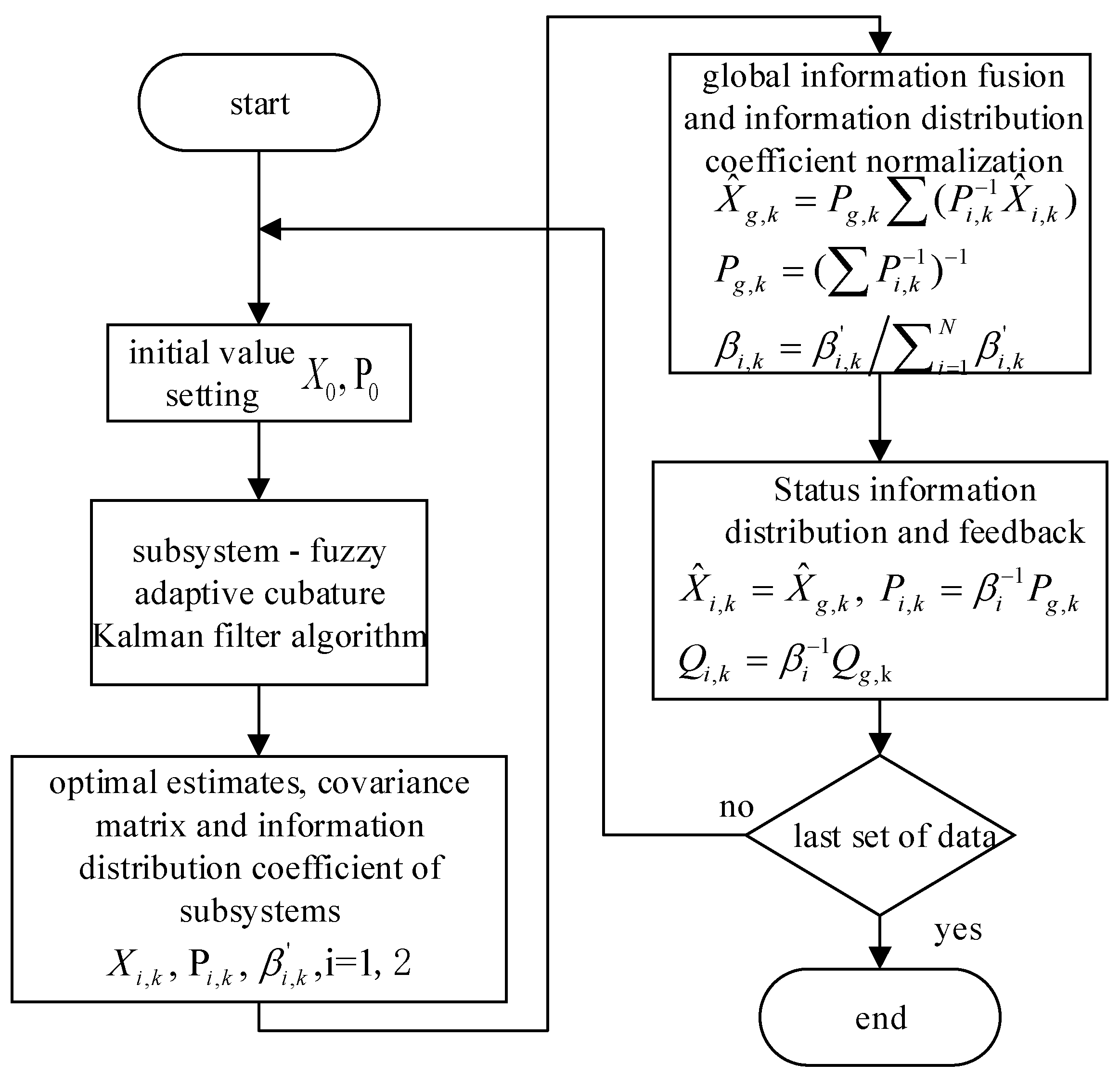
3.1. Improved Cubature Kalman Filter Algorithm

The federal Kalman filter (FKF) belongs to a two-step cascade decentralized filtering, and the core idea is the principle of “information distribution”, i.e., the global state information and the system noise matrix are decentralized and distributed to each sub-filter, and then the local estimation information of each sub-filter is integrated to achieve the optimal fusion estimation by the main filter [25]. This structure does not change the unique form of the sub-filter algorithm, thus making it flexible in design and fault tolerant.

The automobile is a complex nonlinear system, and the CKF solves the nonlinear integrals from the perspective of the monomial exact integration without the need to compute the Jacobi matrix, and it has a greater advantage in estimating high-dimensional nonlinear systems. Therefore, through the comparative analysis of the estimation accuracy, real-time performance, and stability, the federal Kalman filter neutron filter is designed based on the CKF.

During the state estimation process, noise uncertainty is introduced due to factors such as simplification of the system model, sensor measurement errors, or external disturbances. For example, wind force on the vehicle during driving, changes in road friction, tire slip, etc., can cause the system’s variance array Q and R to change. Due to the diversity, variability and complexity of the noise, as well as assumptions about the model and measurements, these assumptions may not fully characterize the true properties of the noise, thus leading to uncertainty about the noise characteristics. According to the characteristics of noise, we reduce the influence of noise on the system state estimation by the design of estimation algorithms to improve the accuracy and precision of the estimation.

In order to improve the adaptability of the filtering algorithm to the observation noise, the fuzzy adaptive is introduced into the CKF. The basic idea is that, in the estimation process, fuzzy reasoning is utilized to adjust R dynamically according to the output adjustment factor, so that the actual value of the residual covariance is consistent with the theoretical value, and the error between the two is reduced as much as possible. Fuzzy mathematics is a method of solving incomplete and imprecise information by utilizing fuzzy theory, and its advantage lies in the fact that it can solve the problem of initiative and fuzziness of human thinking more naturally. At the same time, due to the sub-filter filtering results of good and bad and the related state parameters, the mathematical relationship between the sub-filter results is not certain, showing a certain degree of ambiguity. Therefore, this paper adopts fuzzy logic to adjust the performance of the sub-filter, and then dynamically adjusts the information allocation coefficients according to its filtering confidence. At the same time, according to the filtering effect of the sub-filter, it determines whether it is necessary to carry out adaptive filtering. The detailed steps are as follows.

The residual is the difference between the actual observed value and the estimated value, which is expressed in the nonlinear CKF algorithm as:

$${\eta }_{k+1}=z_{k+1}-{\widehat{z}}_{k+1|k}$$

(15)

The actual residual covariance of the system is:

$$C_{k+1}=\frac{1}{M}{\displaystyle \sum _{i=k-M+2}^{k+1}}{\eta }_{i+1}{\eta }_{i+1}^T$$

(16)

In the formula, M is the smoothing window selected according to experience.

The theoretical residual covariance of the system is:

$$P_{zz,k|k-1}={\displaystyle \sum _{j=1}^m}\frac{1}{m}{Z}_{j,k/k-1}{Z}_{j,k/k-1}^T-Z_{k/k-1}^{^}{Z}_{k/k-1}^{^T}+R$$

(17)

The difference between both is:

$$\alpha =tr(C_{k+1})-tr(P_{zz,k|k-1})$$

(18)

If the observed noise covariance is accurate, the difference between the actual value of the residual covariance and the theoretical value is approximately zero; otherwise, the difference between the two will deviate from zero. The residual covariance can be corrected in real time by adjusting R to keep the filtering stable. The theoretical residual covariance is:

$$P_{zz,k|k-1}={\displaystyle \sum _{j=1}^m}\frac{1}{m}{Z}_{j,k/k-1}{Z}_{j,k/k-1}^T-Z_{k/k-1}^{^}{Z}_{k/k-1}^{^T}+\epsilon R$$

(19)

Among them, $\epsilon$ is the adjustment factor. If the actual value of the observed noise covariance is greater than the theoretical value, the adjustment factor is increased. On the contrary, the correction of R is achieved by reducing the adjustment factor.

The input of the fuzzy system is the difference, $\alpha$, and its derivative, $\dot{\alpha }$, and the output is $\epsilon$. The input and output fuzzy sets of the system are defined as:

$$\begin{array}{l}\alpha =\left\{NB,NM,NS,Z,PS,PM,PB\right\}\\ \dot{\alpha }=\left\{NB,NM,Z,PM,PB\right\}\\ \epsilon =\left\{PVS,PS,PSM,PM,PSB,PMS,PB,PVB\right\}\end{array}$$

The membership functions of input and output are shown in Figure 3 and Figure 4, respectively, and the fuzzy rules are shown in

Table 1. Fuzzy rule table.

$\dot{\mathit{\alpha }}$	$\dot{\mathit{\alpha }}$
	NB	NM	NS	Z	PS	PM	PB
NB	PVB	PB	PMB	PSM	PVS	PS	PMB
NM	PB	PMB	PM	PM	PS	PSM	PB
Z	PMB	PM	PSM	PSM	PSM	PM	PMB
PM	PB	PSM	PS	PM	PM	PMB	PB
PB	PMB	PS	PSM	PMB	PMB	PB	PVB

.

The theoretical residual variance matrix is adjusted by fuzzy reasoning, so that the filtering algorithm can adapt to the uncertain measurement noise, and the estimation accuracy of the algorithm can be improved.

3.2. Research on Adaptive Information Distribution Algorithm

In the federated Kalman filter, the selection of the value of $\beta$ directly affects the filtering accuracy, fault tolerance ability of the system, and the difficulty of calculation in the filtering process, and also has a certain impact on the structure and properties of the federated Kalman filter [16,26,27,28].

In order to study the information distribution coefficient further, the relationship between the sub-filter and the adaptive filter is firstly analyzed. In the adaptive filter, the error of the state model is controlled and adjusted by the adaptive factor, and the cost function is:

$${\nu }_k^T{R}_k^{-1}{\nu }_k+{\alpha }_k{\nu }_{{\overline{X}}_K}^T{P}_{{\overline{X}}_K}^{-1}{\nu }_{{\overline{X}}_K}-2L_k^T(H_k{\widehat{X}}_k-z_k-{\nu }_k)=\min$$

(20)

where

$${\nu }_k=H_k{\widehat{X}}_k-z_k$$

(21)

$${\nu }_{{\overline{X}}_k}={\widehat{X}}_k-{\widehat{X}}_{k|k-1}={\widehat{X}}_k-A_{k|k-1}{\widehat{X}}_{k-1}$$

(22)

In the formula, ${\alpha }_k$ represents the adaptive factor.

The adaptive filtering solution is as follows:

$$\begin{array}{l}{\widehat{X}}_k={\widehat{X}}_{k|k-1}+\frac{1}{{\alpha }_k}{P}_{{\overline{X}}_k}{H}_k^T {(\frac{1}{{\alpha }_k}{H}_k{P}_{{\overline{X}}_k}{H}_k^T+R_k)}^{-1}(z_k-H_k{\widehat{X}}_{k|k-1})\\ ={\widehat{X}}_{k|k-1}+{\overline{G}}_k(z_k-H_k{\widehat{X}}_{k|k-1})\end{array}$$

(23)

where ${\overline{G}}_k$ represents the gain matrix.

The one-step state error covariance matrix of the sub-filter is:

$$\begin{array}{l}{P}_{i,k|k-1}=A_{k|k-1}{P}_{i,k-1}{A}_{k|k-1}^T+Q_{k-1}\\ =A_{k|k-1}\frac{1}{{\beta }_i}{P}_{g,k-1}{A}_{k|k-1}^T+\raisebox{1ex}{$1$}\!\left/ \!\raisebox{-1ex}{${\beta }_i$}\right.Q_{g,k-1}\\ =\frac{1}{{\beta }_i}(A_{k|k-1}{P}_{g,k-1}{A}_{k|k-1}^T+Q_{g,k-1})=\frac{1}{{\beta }_i}{P}_{i,k|k-1}^{\prime }\end{array}$$

(24)

The gain matrix is:

$$\begin{array}{l}{K}_{i,k}=P_{i,k|k-1}{H}_{i,k}^T{(H_{i,k}{P}_{i,k|k-1}{H}_{i,k}^T+R_{i,k})}^{-1}\\ =\raisebox{1ex}{$1$}\!\left/ \!\raisebox{-1ex}{${\beta }_i$}\right.P_{i,k|k-1}^{\prime }{H}_{i,k}^T{(H_{i,k}\raisebox{1ex}{$1$}\!\left/ \!\raisebox{-1ex}{${\beta }_i$}\right.P_{i,k|k-1}^{\prime }{H}_{i,k}^T+R_{i,k})}^{-1}\\ =\raisebox{1ex}{$1$}\!\left/ \!\raisebox{-1ex}{${\beta }_i$}\right.P_{i,k|k-1}^{\prime }{H}_{i,k}^T{(\raisebox{1ex}{$1$}\!\left/ \!\raisebox{-1ex}{${\beta }_i$}\right.H_{i,k}{P}_{i,k|k-1}^{\prime }{H}_{i,k}^T+R_{i,k})}^{-1}\end{array}$$

(25)

After the measurement update, the sub-filter outputs the local state estimate and its error covariance matrix:

$$\begin{array}{l}{\widehat{X}}_{i,k}={\widehat{X}}_{i,k|k-1}+K_{i,k}(z_k-H_{i,k}{\widehat{X}}_{i,k|k-1})\\ ={\widehat{X}}_{i,k|k-1}+\frac{1}{{\beta }_i}{P}_{i,k|k-1}^{\prime }{H}_{i,k}^T\\ {(\frac{1}{{\beta }_i}{H}_{i,k}{P}_{i,k|k-1}^{\prime }{H}_{i,k}^T+R_{i,k})}^{-1}(z_k-H_k{\widehat{X}}_{k|k-1})\end{array}$$

(26)

$$\begin{array}{l}{P}_{i,k}=(I-K_{i,k}{H}_{i,k})P_{i,k|k-1}\\ =\raisebox{1ex}{$1$}\!\left/ \!\raisebox{-1ex}{${\beta }_i$}\right.(I-K_{i,k}{H}_{i,k})P_{i,k|k-1}^{\prime }\end{array}$$

(27)

Compared with Formula (23), if ${\alpha }_k={\beta }_i$,$K_{i,k}={\overline{G}}_k$, the sub-filter of the federated Kalman filter and the adaptive filter are consistent in form.

By substituting the above formula into the federal filter information fusion equation yields, we can obtain:

$$\begin{array}{l}{\widehat{X}}_{g,k}=P_{g,k}{\displaystyle \sum P_{i,k}^{-1}}{\widehat{X}}_{i,k}\\ =P_{g,k}{\displaystyle \sum {\beta }_i{P}_{i,k|k-1}^{\prime }}{(I-K_{i,k}{H}_{i,k})}^{-1}{\widehat{X}}_{i,k|}\end{array}$$

(28)

$$\begin{array}{l}{P}_{g,k}={({\displaystyle \sum P_{i,k}^{-1}})}^{-1}\\ ={(\sum {\beta }_i{P}_{i,k|k-1}^{\prime }{(I-K_{i,k}{H}_{i,k})}^{-1})}^{-1}\end{array}$$

(29)

It can be seen from the above formula that the value of $\beta$ in each sub-filter is proportional to the filtering accuracy. When the accuracy of the sub-filter model is low, the FKF can adjust the system noise matrix and error variance matrix through $\beta$, thereby reducing the error caused by an inaccurate sub-filter. At the same time, since the FKF and the adaptive filter are equivalent in form, $\beta$ can be obtained by referring to the solution method of the adaptive factor. Based on this, the construction of the adaptive federal filter is completed, and the accuracy of the sub-filter is improved, while retaining the advantages of the federal filter.

In most cases, the error of the kinematic model can be measured by the size of the predicted residual vector, $e_k$, so the adaptive factor can be solved according to the predicted residual.

If the system model is accurate and the current measurement information is reliable, then:

$$e_k\sim N(0,H_k{P}_{k|k-1}{H}_k^T+R_k)$$

(30)

Based on the characteristic that the residuals satisfy the normal distribution, construct a new statistic:

$${\gamma }_k=\frac{e_k{e}_k^T}{tr(H_k{P}_{k|k-1}{H}_k^T+R_k)}$$

(31)

Therefore, the adaptive solution formula for the information distribution factor is:

$${\beta }_k^{\prime }=\left\{\begin{array}{c}1, \left|{\gamma }_k\right|\le c\\ c/\left|{\gamma }_k\right|, \left|{\gamma }_k\right|>c\end{array}\right.$$

(32)

In the formula, $c$ represents a fixed value, and the general value is $c=0.85\sim 1$.

${\gamma }_k$ is used to determine the state of the current sub-filter. If $\left|{\gamma }_k\right|>c$, it means that there is an abnormality in the observation information, then ${\beta }_k^{\prime }=c/\left|{\gamma }_k\right|$, and its value feeds back the error of the sub-filter at the current moment. Conversely, if $\left|{\gamma }_k\right|<c$, then ${\beta }_k^{\prime }=1$. This is because the system model is accurate and the observation information is reliable in the current state, and the local estimation performance of the sub-filter is good.

The adaptive factor is normalized, as follows:

$${\beta }_{i,k}=\frac{{\beta }_{i,k}^{\prime }}{{\displaystyle {\sum }_{i=1}^N{\beta }_{i,k}^{\prime }}}$$

(33)

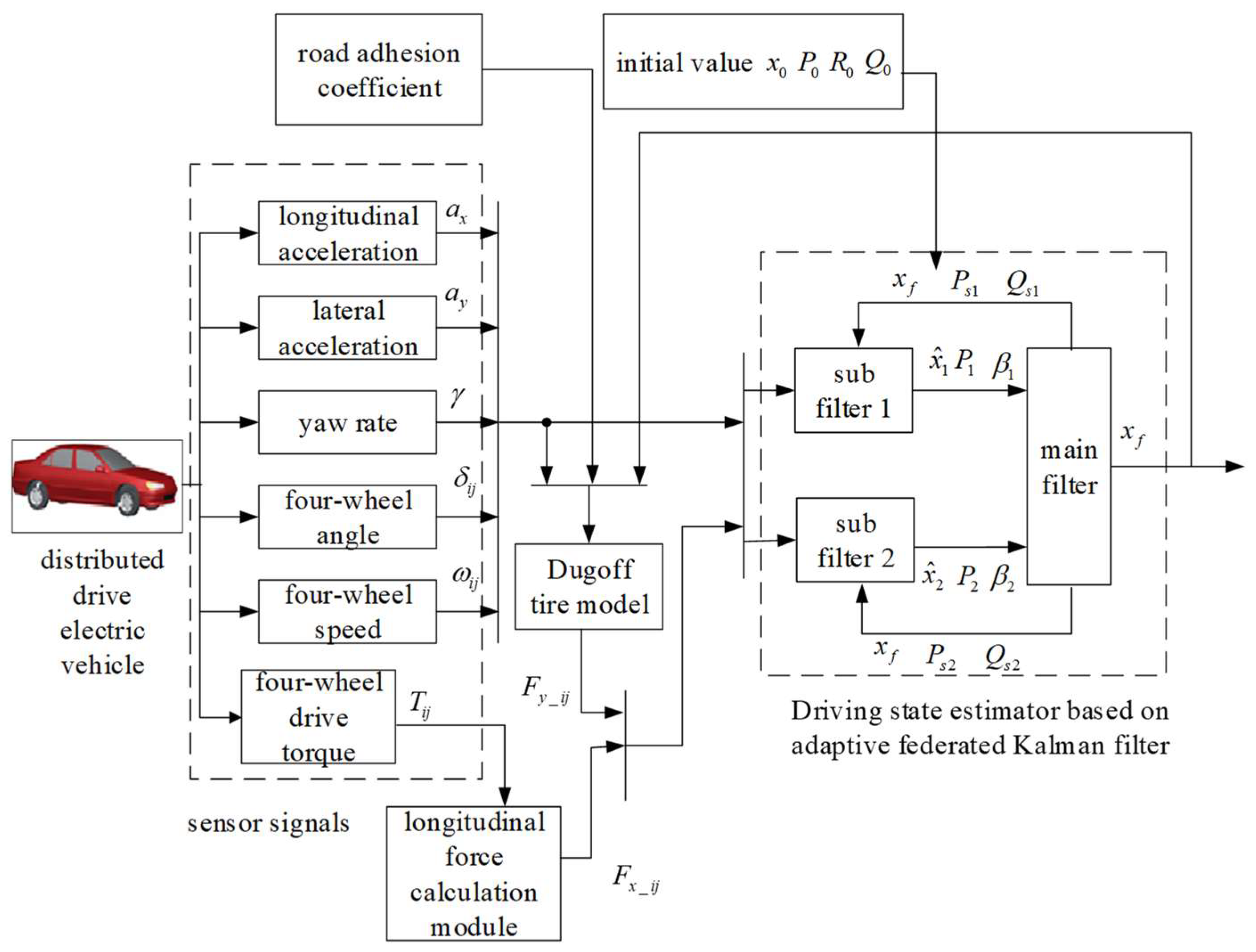
4. Driving State Estimation for Distributed Drive Electric Vehicles

4.1. Principle of Vehicle Traveling State Estimation

The estimation principle of the driving state of the distributed drive electric vehicle is shown in Figure 5.

The main process is: firstly, the on-board sensors are applied to obtain the required information and pass it as input to the vehicle driving state estimator and the Dugoff tire model. Then, the set road adhesion coefficient is input into the tire model, and, at the same time, the tire model calculates the input information to obtain the lateral force of the tire. In order to reduce the error caused by the model, the unique advantages of four-wheel independent drive and four-wheel independent steering are used to convert the four-wheel drive torque directly to obtain the longitudinal force of the tire, which is transmitted as an input to the vehicle driving state estimator. Finally, the driving state estimator obtains the global optimal estimated value through the four processes of information allocation, time update, measurement update, and information fusion. At the same time as the output, the global optimal estimated value will also continuously revise the tire model through feedback, thus forming a complete closed-loop feedback system. As time increases, the iterative process is completed again and again to achieve accurate estimates of longitudinal and lateral velocities, as well as centroid slip angle.

4.2. Estimation Process

The state equation and measurement equation are:

$$\begin{array}{l}{X}_{si,k}=f\left(X_{si,k-1},U_{si,k-1},W_{si,k-1}\right)\\ \begin{array}{cc}& \end{array} Z_{si,k}=h\left(X_{si,k},v_{si,k}\right)\end{array}$$

(34)

The state variables are: $X_{si,k}=[u,v,a_x,a_y,\gamma ,\Gamma ]$.

The measured variables of the two sub-filters are: $Z_{s1,k}=[a_x,a_y,\gamma ]$,$Z_{s1,k}=[a_y,\gamma ]$.

The control input variables are: $U_{s,k}=[{\delta }_{fl},{\delta }_{fr},{\delta }_{rl},{\delta }_{rr},{\omega }_{fl},{\omega }_{fr},{\omega }_{rl},{\omega }_{rr}]$.

The specific implementation steps of the method for estimating the driving state of the vehicle are as follows:

Step 1. Distribution of information in the main filter.

$$X_{{}_{si,k-1}}^{^}=X_{sf,k-1}$$

(35)

$$P_{si,k-1}^{-1}={\beta }_{si}{P}_{sf,k-1}^{-1}$$

(36)

$$Q_{si,k-1}^{-1}={\beta }_{si}{Q}_{sf,k-1}^{-1}$$

(37)

Step 2. Time update of localized filters.

Select the singular value decomposition method (SVD) to decompose the error covariance matrix, and calculate the cubature points:

$$P_{s,k-1}=A_{s,k-1}{\mathrm{\Lambda }}_{s,k-1}{A}_{s,k-1}^T$$

(38)

$$X_{sj,k-1}=A_{si,k-1}{S}_{si,k-1}{\xi }_j+X_{s,k-1}^{^}$$

(39)

The driving state variable in the paper is 6, then the corresponding cubature point set is expressed as:

$$\left\{\left[\begin{array}{l}1\\ 0\\ 0\\ 0\\ 0\\ 0\end{array}\right],\left[\begin{array}{l}0\\ 1\\ 0\\ 0\\ 0\\ 0\end{array}\right],\left[\begin{array}{l}0\\ 0\\ 1\\ 0\\ 0\\ 0\end{array}\right],\left[\begin{array}{l}0\\ 0\\ 0\\ 1\\ 0\\ 0\end{array}\right],\left[\begin{array}{l}0\\ 0\\ 0\\ 0\\ 1\\ 0\end{array}\right],\left[\begin{array}{l}0\\ 0\\ 0\\ 0\\ 0\\ 1\end{array}\right],\left[\begin{array}{l}-1\\ 0\\ 0\\ 0\\ 0\\ 0\end{array}\right],\left[\begin{array}{l}0\\ -1\\ 0\\ 0\\ 0\\ 0\end{array}\right],\left[\begin{array}{l}0\\ 0\\ -1\\ 0\\ 0\\ 0\end{array}\right],\left[\begin{array}{l}0\\ 0\\ 0\\ -1\\ 0\\ 0\end{array}\right],\left[\begin{array}{l}0\\ 0\\ 0\\ 0\\ -1\\ 0\end{array}\right],\left[\begin{array}{l}0\\ 0\\ 0\\ 0\\ 0\\ -1\end{array}\right]\right\}$$

Obtain a new cubature point through the system state transition model function:

$$X_{sj,k/k-1}^{\ast }=f\left(X_{sj,k/k-1},U_k\right)$$

(40)

The predicted value of the one-step state is:

$$X_{s,k/k-1}^{^}={\displaystyle \sum _{j=1}^m}\frac{1}{m}{X}_{sj,k/k-1}^{\ast }$$

(41)

The predicted value of the one-step error covariance matrix is:

$$P_{s,k/k-1}={\displaystyle \sum _{j=1}^m}\frac{1}{m}{X}_{sj,k/k-1}^{\ast }{X}_{sj,k/k-1}^{\ast T}-X_{s,k/k-1}^{^}{X}_{s,k/k-1}^{^T}+Q_s$$

(42)

where $Q_s$ is the process noise covariance matrix of the system.

Step 3. Measurement update of localized filters.

Calculate the cubature point:

$$P_{s,k/k-1}=A_{s,k/k-1}{\Lambda }_{s,k/k-1}{A}_{s,k/k-1}^T$$

(43)

$$X_{sj,k/k-1}=A_{si,k/k-1}{S}_{si,k/k-1}{\xi }_j+X_{s,k/k-1}^{^}$$

(44)

Substitute into the measurement model function to obtain a new cubature point:

$$Z_{sj,k/k-1}=h\left(X_{sj,k/k-1},X_{sj,k/k-1}^{^},U\left(k\right)\right)$$

(45)

Calculate the mean:

$$Z_{sj,k/k-1}^{^}={\displaystyle \sum _{j=1}^m}\frac{1}{m}{Z}_{sj,k/k-1}$$

(46)

The input to the fuzzy controller with its derivatives and the output regulation factor are calculated by fuzzy rules.

Calculate the adjusted new interest variance according to Equation (19).

The cross-covariance is:

$$P_{sxz,k/k-1}={\displaystyle \sum _{j=1}^m}\frac{1}{m}{X}_{sj,k/k-1}{Z}_{sj,k/k-1}^T-X_{s,k/k-1}^{^}{Z}_{s,k/k-1}^{^T}$$

(47)

The filter gain is:

$$K_{s,k}=P_{sxz,k/k-1}{P}_{szz,k/k-1}^{-1}$$

(48)

The updated error covariance matrix and state estimate are:

$$P_{s,k}=P_{s,k/k-1}-K_{s,k}{P}_{szz,k/k-1}{K}_{s,k}^T$$

(49)

$$X_{s,k}^{^}=X_{s,k/k-1}^{^}+K_{s,k}(Z_{s,k}-Z_{s,k/k-1}^{^})$$

(50)

The adaptive information allocation factor for each sub-filter is calculated from Equations (31) and (32).

Step 4. Information fusion for main filters: obtain the global optimal state estimate and error covariance matrix. Normalize the information allocation factor according to Equation (33).

$$P_{sf,k}^{-1}=P_{s1,k}^{-1}+P_{s2,k}^{-1}$$

(51)

$$X_{sf,k}^{^}=P_{sf,k}^{-1}\left(P_{s1,k}^{-1}{X}_{s1,k}^{^}+P_{s2,k}^{-1}{X}_{s2,k}^{^}\right)$$

(52)

The complete algorithm flow chart is given according to the above algorithm steps, as shown in Figure 6.

4.3. Simulation Verification

On the basis of the original model in CarSim, the whole vehicle model of the distributed drive electric vehicle is built by setting the parameters of the real vehicle and connecting the motor model. The main parameters of the real car are shown in

Table 2. Main parameters of vehicle model.

Symbol	Parameter Name	Value
m	Vehicle mass (kg)	830
m	Sprung mass (kg)	747
L	Wheelbase (m)	2.34
A	Distance from center of mass to front axle (m)	1.17
d1	Front wheel track (m)	1.416
d2	Rear wheel track (m)	1.416
r	Wheel radius (m)	0.278
h	Distance from the centroid to ground (m)	0.54
Iz	Rotational inertia (kg·m2)	1110

.

In the four-wheel proportional control strategy, the proportional coefficient is a function related to vehicle speed [29], as shown in Formula (53).

$$k=\frac{{\delta }_r}{{\delta }_f}=\frac{-b+[\frac{ma}{k_2(a+b)}]u^2}{a+[\frac{mb}{k_1(a+b)}]u^2}$$

(53)

Three experimental conditions with different road adhesion coefficients are selected, and simulation experiments are carried out to verify the vehicle driving state estimation algorithm based on the federated Kalman filter and the improved filter design, respectively.

• High-adhesion road conditions.

These conditions require that the road surface has good adhesion properties, and the vehicle speed should be selected as an appropriate value to prevent the vehicle from skidding and rollover during the simulation process, which can verify the response characteristics of the algorithm in extreme conditions. The experimental condition is the double line-shifting condition, with a road adhesion coefficient of 0.85. The initial vehicle speed is set to 40 km/h, and the sampling time is set to a fixed value of 0.02 s.

The setting of the initial value in the driving state estimation algorithm is:

$$\begin{array}{l}{X}_0=[40/3.6,0,0,0,0,0] P_{s1,0}=\mathrm{diag}\left(\right[1,1,1,1,1,1\left]\right) P_{s2,0}=\mathrm{diag}\left(\right[1,1,1,1,1,1\left]\right)\\ Q_{s1,0}=\mathrm{diag}\left(\right[1,1,1,1,1,1\left]\right)\ast 0.01 Q_{s2,0}=\mathrm{diag}\left(\right[1,1,1,1,1,1\left]\right)\ast 0.01\\ R_{s1.0}=\mathrm{diag}\left(\right[0.01,100,1\left]\right)\ast 0.1 R_{s2.0}=\mathrm{diag}\left(\right[0.1,10\left]\right)\ast 0.01 \end{array}$$

(54)

Figure 7 is a graph of the comparison between the estimated value of the vehicle’s driving state and the actual value obtained by the federated Kalman filter and the improved algorithm. Due to the low speed of the current vehicle, in order to reduce the turning radius of the vehicle and improve the passing ability of the vehicle, the four-wheel angles are turned in opposite directions. Figure 7a is the comparison curve of longitudinal vehicle speed. It can be seen from the curve that the maximum error of the estimation result based on adaptive Kalman filtering is about 0.1%, which has good tracking ability and real-time performance, and the estimation accuracy is significantly higher than that of the FKF. Figure 7b,c are the comparison curves between the estimated and actual values of the lateral vehicle speed and centroid slip angle, respectively. It can be clearly seen from the curve that the estimated value obtained by the improved algorithm is basically consistent with the actual value, and there is a small error at the peak and valley. However, the overall estimation effect is good, and the error remains within a reasonable range. In contrast, there is a large error between the estimated value obtained by the federated Kalman filter algorithm and the actual value, and the estimated value has obvious disadvantages in tracking effect, estimation accuracy, real-time performance, and convergence trend.

In order to compare the errors of the two algorithms quantitatively, the mean absolute error (MAE) and root mean square error (RMSE) of the estimated value relative to the true value are calculated, as shown in

Table 3. MAE and RMSE indicators of the simulation results of the two algorithms.

	MAE		RMSE
Estimated Parameters	FKF Algorithm	Improved Algorithm	FKF Algorithm	Improved Algorithm
Longitudinal speed vx (m/s)	0.0050	0.0009	0.0063	0.0012
Lateral speed vy (m/s)	0.0274	0.0024	0.0572	0.0040
Centroid slip angle $\beta$ (deg)	0.0025	0.0002	0.0051	0.0004

, and the calculation method is referred to [30].

From Table 3, it can be seen more intuitively that the estimation error of the vehicle driving state obtained by the improved algorithm is smaller, and it has more advantages in accuracy than the estimation algorithm designed based on the federated Kalman filter theory.

• Medium-adherent pavement conditions.

The initial vehicle speed is set to 70 km/h, and the road adhesion coefficient is set to 0.5. During the simulation process, the steering wheel is input with a sinusoidal angle signal, which can verify the adaptability and accuracy of the algorithm under continuous turning conditions.

The selection of the initial value in the driving state estimation algorithm is:

$$\begin{array}{l}{X}_{s,0}=[70/3.6,0,0,0,0,0] P_{s1,0}=\mathrm{diag}\left(\right[1,1,1,1,1,1\left]\right) P_{s2,0}=\mathrm{diag}\left(\right[1,1,1,1,1,1\left]\right)\\ Q_{s1,0}=\mathrm{diag}\left(\right[1,1,1,1,1,1\left]\right) Q_{s2,0}=\mathrm{diag}\left(\right[1,1,1,1,1,1\left]\right)\\ R_{s1.0}=\mathrm{diag}\left(\right[0.01,1,1\left]\right)\ast 0.1 R_{s2.0}=\mathrm{diag}\left(\right[0.1,0.1\left]\right)\ast 0.001 \end{array}$$

(55)

Figure 8 is a graph showing the comparison between the estimated value of the driving state and the actual value obtained using the federated Kalman filter and the improved estimation algorithm. Among them, Figure 8a is the comparison curve of the longitudinal vehicle speed. It can be seen from the curve in the figure that the estimation results of the two algorithms have relatively large errors when the steering wheel angle reaches the maximum. However, the estimated value obtained by the improved algorithm is closer to the actual value, and its overall estimation accuracy and stability are relatively better. Figure 8b,c are the comparison curves of the lateral vehicle speed and centroid side slip angle, respectively. It can be seen that simulation results obtained by the improved algorithm almost coincide with the real value curves. Tracking consistency is maintained during continuous cornering maneuvers, even when the steering wheel inputs a sinusoidal signal. Compared with the estimation result of the federated Kalman filter algorithm, it has more advantages in accuracy, and also maintains a good estimation effect in terms of real time and stability.

• Low-adhesion road conditions.

As the experimental condition was selected as a serpentine condition with a road adhesion coefficient of 0.3, the vehicle speed was also selected to be smaller to adapt to the road surface to prevent the vehicle from skidding and tailgating, and the initial vehicle speed was set to 30 km/h.

The initial value of the driving state estimation algorithm is selected as:

$$\begin{array}{l}{X}_{s,0}=[30/3.6,0,0,0,0,0]\\ P_{s1,0}=eye(6)\ast 100 P_{s2,0}=eye(6)\ast 100\\ Q_{s1,0}=eye(6) Q_{s2,0}=eye(6)\\ R_{s1.0}=\mathrm{eye}\left(3\right)\ast 0.001 R_{s2.0}=\mathrm{eye}\left(2\right)\ast 5\end{array}$$

(56)

Figure 9 shows the comparison of the estimated value and the actual value obtained by the federated Kalman filter and the improved algorithm, respectively. Figure 9a shows the simulation results of the longitudinal vehicle speed. It can be seen from the curve that, in the case of complex actual vehicle speed changes, the error of the estimated value obtained based on the federated Kalman filter algorithm increases with time, and gradually deviates from the true value in the later stage, and its stability is relatively poor. The state estimation value obtained by the improved algorithm can still follow the real value, and the error slightly increases with time, but remains within a reasonable range. Figure 9b,c are the comparison curves of the simulation results of the lateral vehicle speed and the centroid side slip angle, respectively. The estimated values obtained by the two estimation algorithms can track the actual values very well. The simulation results obtained based on the federated Kalman filter theory have a good fit within the first 8 s, and, with the increase in time, a small error gradually appears, and the error is the largest at the peak. However, the estimated value obtained by the improved algorithm basically coincides with the actual value curve, and a good fitting effect is also maintained at the peak. It can be proved that the improved adaptive Kalman filter algorithm based on the federated Kalman filter theory is feasible, and has more advantages in accuracy, stability, and real-time performance.

5. Hardware-in-the-Loop Experimental Verification

The validity and estimation accuracy of the designed algorithm are further verified based on the driving simulator experimental platform. Among them, the input signals of the target vehicle and the state estimation algorithm are provided by the real driver’s operating device, which mainly includes signals such as steering wheel angle, driving pedal, and brake pedal. During the simulation process, the driver needs to control the vehicle in real time through the dynamic road information displayed on the ring screen, based on subjective judgment and actual research, so it is difficult to ensure that the vehicle is in a constant speed, which further verifies the adaptability of the algorithm. Subject to the limitations of real driver maneuvering, two typical experimental conditions, double-shift line and snake, are selected for hardware-in-the-loop real-time simulation experiments.

• Variable speed double-shift line experimental conditions.

The double-shifted line surface was set up in CarSim, with its attachment factor set to 0.9. The selection of the initial value in the driving state estimation algorithm is:

$$\begin{array}{l}{X}_{s0}=[4/3.6,0,0,0,0,0]\\ P_{s1,0}=\mathrm{diag}\left(\right[1,1,1,1,1,1\left]\right) P_{s2,0}=\mathrm{diag}\left(\right[1,1,1,1,1,1\left]\right)\\ {\mathrm{Q}}_{s1,0}=\mathrm{diag}\left(\right[1,1,1,1,1,1\left]\right) Q_{s2,0}=\mathrm{diag}\left(\right[1,1,1,1,1,1\left]\right)\\ R_{s1.0}=\mathrm{diag}\left(\right[0.001,1,5\left]\right)\ast 0.1 R_{s2.0}=\mathrm{diag}\left(\right[0.1,1\left]\right)\ast 0.01\end{array}$$

(57)

Figure 10 is the comparison curve between the estimated value obtained by the vehicle driving state estimation algorithm and the actual value output of the vehicle simulation model. Figure 10a is a comparison curve of the longitudinal vehicle speed under double-lane-shifting conditions. It can be seen from the curve that the estimated value of the longitudinal speed is basically consistent with the actual value curve, and, even if the vehicle is in a continuous acceleration state, it can be tracked very well. Figure 10b,c are the comparison curves of the lateral vehicle speed and the centroid side slip angle, respectively. The estimated results of the two are generally consistent with the actual values, and the curves are basically consistent within 0–11 s, and the tracking effect at the peak is also good.

• Variable speed serpentine experimental conditions.

Set up the serpentine pavement in CarSim and set its pavement adhesion coefficient to 0.9. The selection of the initial value in the driving state estimation algorithm is:

$$\begin{array}{l}{X}_{s0}=[4.68/3.6 0 0 0 0 0]\\ P_{s1,0}=\mathrm{eye}\left(4\right)\ast 10 P_{s2,0}=\mathrm{eye}\left(4\right)\ast 10\\ Q_{s1,0}=eye(4) Q_{s2,0}=eye(4)\\ R_{s1.0}=\mathrm{diag}\left(\right[0.01,1,5\left]\right)\ast 0.1 R_{s2.0}=\mathrm{diag}\left(\right[0.1,1\left]\right)\ast 0.01\end{array}$$

(58)

Figure 11 shows the comparison curves of the estimated values of the longitudinal/lateral speed and center-of-mass lateral deflection angle obtained using the adaptive Kalman filter algorithm with the real values of the actual output of the simulation. Figure 11a shows the comparison curve of the longitudinal speed, and the curve shows that the two are basically in a synchronized state, indicating that the joint algorithm maintains a good estimation accuracy of the longitudinal speed estimation and has good real time and stability. Figure 11b,c show the comparison curves of lateral velocity and center-of-mass lateral deflection, respectively. It can be seen that, when the longitudinal velocity is in a lower state, the estimated values of lateral velocity and center-of-mass lateral deflection track the actual values better. With the increasing of longitudinal velocity, there is a small error between the estimated and actual values of the two, and, especially when the values reach the peak or the bottom, the deviation is more obvious, but they are all in a reasonable range, which is in line with the requirements of the actual project.

6. Conclusions

This paper takes the distributed electric drive vehicle as the research object, and at the same time considers the influence of road surface information, combines the estimation model of the vehicle, takes the adaptive Kalman filter as the theoretical support to design the vehicle driving state estimation algorithm, and realizes the accurate estimation of the driving state information. In order to improve the estimation accuracy of the algorithm, as well as the adaptability to the observation noise, the sub-filter of the federal Kalman filter adds a fuzzy controller on the basis of the volumetric Kalman filter to realize the adaptive adjustment of the statistical characteristics of the observation noise. At the same time, the information allocation coefficient is dynamically adjusted by combining the solution method of the adaptive factor to improve the fault-tolerance performance of the algorithm.

After experimental comparison and verification, the estimation algorithm designed in this paper has obvious advantages in terms of estimation accuracy and real-time performance, and achieves the expected results. However, due to the limitations of time, experimental conditions, and other factors, there are still shortcomings, and more in-depth research can be carried out subsequently:

(1)

In order to reduce the error caused by the model accuracy during the filtering process, and to make the model closer to reality, more degrees of freedom can be considered to be built.

(2)

Due to the limited authorization of experimental equipment and experimental sites, the algorithms involved have not been studied in depth in different initial states and real urban road scenes, and it is necessary to carry out real vehicle experiments under multiple working conditions to improve the adaptability and accuracy of the algorithms under actual driving conditions in future research.

(3)

In this paper, the design of the estimation algorithm is carried out on a distributed drive electric vehicle, which can be applied to other types of vehicles in the future to verify the portability of the algorithm.

References

1. Hooftman, N.; Oliveira, L.; Messagie, M.; Coosemans, T.; Van Mierlo, J. Environmental Analysis of Petrol, Diesel and Electric Passenger Cars in a Belgian Urban Setting. Energies 2016, 9, 84. [Google Scholar] [CrossRef]
2. Jochem, P.; Doll, C.; Fichtner, W. External costs of electric vehicles. Transp. Res. Part D Transp. Environ. 2016, 42, 60–76. [Google Scholar] [CrossRef]
3. Katsuyama, E.; Yamakado, M.; Abe, M. A state-of-the-art review: Toward a novel vehicle dynamics control concept taking the drive line of electric vehicles into account as promising control actuators. Veh. Syst. Dyn. 2021, 59, 976–1025. [Google Scholar] [CrossRef]
4. Chan, C. Renaissance and Electric Vehicles Development. In Mobility Engineering: Proceedings of CAETS 2015 Convocation on Pathways to Sustainability; Springer: Singapore, 2017; pp. 1–9. [Google Scholar]
5. Sun, C.; Sun, P.; Zhou, J.; Mao, J. Travel reduction control of distributed drive electric agricultural vehicles based on multi-information fusion. Agriculture 2022, 12, 70. [Google Scholar] [CrossRef]
6. Yao, Y.; Yan, Y.; Peng, L.; Han, D.; Wang, J.; Yin, G. Longitudinal and Lateral Coordinated Control of Distributed Drive Electric Vehicles Based on Model Predictive Control. In Proceedings of the 2022 6th CAA International Conference on Vehicular Control and Intelligence (CVCI), Nanjing, China, 28–30 October 2022; pp. 1–6. [Google Scholar]
7. Arndt, M.; Ding, E.; Massel, T. Observer based diagnosis of roll rate sensor. In Proceedings of the 2004 American Control Conference, Boston, MA, USA, 30 June–2 July 2004; pp. 1540–1545. [Google Scholar]
8. Yang, K.; Dong, D.; Ma, C.; Tian, Z.; Chang, Y.; Wang, G. Stability control for electric vehicles with four in-wheel-motors based on sideslip angle. World Electr. Veh. J. 2021, 12, 42. [Google Scholar] [CrossRef]
9. Chu, W. State Estimation and Coordinated Control for Distributed Electric Vehicles; Springer: Berlin/Heidelberg, Germany, 2015. [Google Scholar]
10. Pei, X.; Chen, Z.; Yang, B.; Chu, D. Estimation of states and parameters of multi-axle distributed electric vehicle based on dual unscented Kalman filter. Sci. Prog. 2020, 103, 0036850419880083. [Google Scholar] [CrossRef] [PubMed]
11. Marco, V.R.; Kalkkuhl, J.; Raisch, J. EKF for simultaneous vehicle motion estimation and IMU bias calibration with observability-based adaptation. In Proceedings of the 2018 Annual American Control Conference (ACC), Milwaukee, WI, USA, 27–29 June 2018; pp. 6309–6316. [Google Scholar]
12. Liu, Y.-H.; Li, T.; Yang, Y.-Y.; Ji, X.-W.; Wu, J. Estimation of tire-road friction coefficient based on combined APF-IEKF and iteration algorithm. Mech. Syst. Signal Process. 2017, 88, 25–35. [Google Scholar] [CrossRef]
13. Wenzel, T.A.; Burnham, K.; Blundell, M.; Williams, R. Dual extended Kalman filter for vehicle state and parameter estimation. Veh. Syst. Dyn. 2006, 44, 153–171. [Google Scholar] [CrossRef]
14. Liu, W.; He, H.; Sun, F. Vehicle state estimation based on minimum model error criterion combining with extended Kalman filter. J. Frankl. Inst. 2016, 353, 834–856. [Google Scholar] [CrossRef]
15. Yu, H.; Duan, J.; Taheri, S.; Cheng, H.; Qi, Z. A model predictive control approach combined unscented Kalman filter vehicle state estimation in intelligent vehicle trajectory tracking. Adv. Mech. Eng. 2015, 7, 1687814015578361. [Google Scholar] [CrossRef]
16. Cheng, S.; Li, L.; Chen, J. Fusion algorithm design based on adaptive SCKF and integral correction for side-slip angle observation. IEEE Trans. Ind. Electron. 2017, 65, 5754–5763. [Google Scholar] [CrossRef]
17. Wan, W.; Feng, J.; Song, B.; Li, X. Huber-Based Robust Unscented Kalman Filter Distributed Drive Electric Vehicle State Observation. Energies 2021, 14, 750. [Google Scholar] [CrossRef]
18. Ge, P.; Zhang, C.; Zhang, T.; Guo, L.; Xiang, Q. Maximum Correntropy Square-Root Cubature Kalman Filter with State Estimation for Distributed Drive Electric Vehicles. Appl. Sci. 2023, 13, 8762. [Google Scholar] [CrossRef]
19. Liu, Y.; Cui, D. Estimation algorithm for vehicle state estimation using ant lion optimization algorithm. Adv. Mech. Eng. 2022, 14, 16878132221085839. [Google Scholar] [CrossRef]
20. Kobayashi, T.; Sugiura, H.; Ono, E.; Katsuyama, E.; Yamamoto, M. Efficient direct yaw moment control of in-wheel motor vehicle. In Advanced Vehicle Control; CRC Press: Boca Raton, FL, USA, 2016; pp. 631–636. [Google Scholar]
21. Leng, B.; Jin, D.; Xiong, L.; Yang, X.; Yu, Z. Estimation of tire-road peak adhesion coefficient for intelligent electric vehicles based on camera and tire dynamics information fusion. Mech. Syst. Signal Process. 2021, 150, 107275. [Google Scholar] [CrossRef]
22. Zhang, L.; Chen, H.; Huang, Y.; Wang, P.; Guo, K. Human-centered torque vectoring control for distributed drive electric vehicle considering driving characteristics. IEEE Trans. Veh. Technol. 2021, 70, 7386–7399. [Google Scholar] [CrossRef]
23. Heidfeld, H.; Schünemann, M. Optimization-based tuning of a hybrid ukf state estimator with tire model adaption for an all wheel drive electric vehicle. Energies 2021, 14, 1396. [Google Scholar] [CrossRef]
24. Chindamo, D.; Lenzo, B.; Gadola, M. On the vehicle sideslip angle estimation: A literature review of methods, models, and innovations. Appl. Sci. 2018, 8, 355. [Google Scholar] [CrossRef]
25. Luo, Q.; Yan, X.; Wang, C.; Shao, Y.; Zhou, Z.; Li, J.; Hu, C.; Wang, C.; Ding, J. A SINS/DVL/USBL integrated navigation and positioning IoT system with multiple sources fusion and federated Kalman filter. J. Cloud Comput. 2022, 11, 18. [Google Scholar] [CrossRef]
26. Liu, W.; Liu, Y.; Bucknall, R. A robust localization method for unmanned surface vehicle (USV) navigation using fuzzy adaptive Kalman filtering. IEEE Access 2019, 7, 46071–46083. [Google Scholar] [CrossRef]
27. Huang, B.; Fu, X.; Wu, S.; Huang, S. Calculation algorithm of tire-road friction coefficient based on limited-memory adaptive extended Kalman filter. Math. Probl. Eng. 2019, 2019, 1056269. [Google Scholar] [CrossRef]
28. Zhi-qiang, L.; Yi-qun, L. Estimation algorithm for road adhesion coefficient using adaptive fading unscented Kalman filter. China J. Highw. Transp. 2020, 33, 176. [Google Scholar]
29. Zhao, W.; Qin, X.; Wang, C. Yaw and lateral stability control for four-wheel steer-by-wire system. IEEE/ASME Trans. Mechatron. 2018, 23, 2628–2637. [Google Scholar] [CrossRef]
30. Regression Evaluation Indicators MSE, RMSE, MAE, R-Squared. Available online: https://blog.csdn.net/skullFang/article/details/79107127 (accessed on 19 January 2018).
Figure 1. The vehicle dynamic model.
Sustainability 15 13446 g001
Figure 2. The tire characteristic diagram: (a) tire longitudinal slip characteristic diagram; (b) tire cornering characteristic diagram.
Sustainability 15 13446 g002
Figure 3. Input membership function: (a) the membership function of the input α ; (b) the membership function of the input α ˙ .
Sustainability 15 13446 g003
Figure 4. Output membership function.
Sustainability 15 13446 g004
Figure 5. The schematic diagram of driving state estimation.
Sustainability 15 13446 g005
Figure 6. Flow chart of adaptive federated Kalman filter algorithm.
Sustainability 15 13446 g006
Figure 7. Comparison of simulation results of two vehicle driving state estimation algorithms: (a) comparison of actual output and estimated value of longitudinal speed; (b) comparison of actual output and estimated value of lateral speed; (c) comparison of actual output and estimated value of centroid side slip angle.
Sustainability 15 13446 g007
Figure 8. Comparison of simulation results of two vehicle driving state estimation algorithms: (a) comparison of actual output and estimated value of longitudinal speed; (b) comparison of actual output and estimated value of lateral speed; (c) comparison of actual output and estimated value of centroid side slip angle.
Sustainability 15 13446 g008aSustainability 15 13446 g008b
Figure 9. Comparison of simulation results of two vehicle driving state estimation algorithms: (a) comparison of actual output and estimated value of longitudinal speed; (b) comparison of actual output and estimated value of lateral speed; (c) comparison of actual output and estimated value of centroid side slip angle.
Sustainability 15 13446 g009
Figure 10. Simulation results of joint estimation algorithm: (a) comparison of actual output and estimated value of longitudinal speed; (b) comparison of actual output and estimated value of lateral speed; (c) comparison of actual output and estimated value of centroid side slip angle.
Sustainability 15 13446 g010
Figure 11. Simulation results of joint estimation algorithm: (a) comparison of actual output and estimated value of longitudinal speed; (b) comparison of actual output and estimated value of lateral speed; (c) comparison of actual output and estimated value of centroid side slip angle.
Sustainability 15 13446 g011