Analysis of Machine Learning Models for Wastewater Treatment Plant Sludge Output Prediction

Abstract

With China’s significant investment in wastewater treatment plants, urban sewage is effectively collected and treated, resulting in a substantial byproduct—sludge. As of 2021, a total of 2827 wastewater treatment plants have been constructed across 31 provinces, municipalities, and autonomous regions in China, with a processing capacity of 60.16 billion cubic meters. The production of dry sludge amounts to 14.229 million tons. The treatment and utilization of sludge pose significant challenges. The scientific calculation of sludge production is the basis for the reduction at the source and the design of sludge treatment and energy utilization. It is directly related to the construction scale, structure size, and equipment selection of the sludge treatment and utilization system and affects the operation and environmental management of the sludge treatment system. The wastewater treatment process using microbial metabolism is influenced by various known and unknown parameters, exhibiting highly nonlinear characteristics. These complex characteristics require the use of mathematical modeling for simulations and control. In this study, nine types of machine learning algorithms were used to establish sludge production prediction models. The extreme gradient boosting tree (XGBoost) and random forest models had the best prediction accuracies, with the former having RMSE, MAE, MAPE, and R² values of 4.4815, 2.1169, 1.7032, 0.0415, and 0.8218, respectively. These results suggested a superiority of ensemble learning models in fitting highly nonlinear data. In addition, the contribution and influence of various input features affecting sludge output were also studied for the XGBoost model, and the daily wastewater inflow volume and surrounding temperature features had the greatest impact on sludge production. The innovation of this study lies in the application of machine learning algorithms to achieve the prediction of sludge production in wastewater treatment plants.

1. Introduction

With the rapid development of wastewater treatment facilities in China, the amount of sludge being produced annually has been increasing. In 2021, the amount of dry urban sludge in China reached 14,229,015 tons [1], posing a huge challenge in terms of its treatment and utilization. The scientific calculation of sludge production is the basis for the reduction at source and the design of sludge treatment and energy utilization. It is directly related to the construction scale, structure size, and equipment selection of the sludge treatment and utilization system, and affects the operation and environmental management of the sludge treatment system [2].

At present, the ‘Technical Specifications for Application and Issuance of Pollutant Discharge Permit’ [3] for the water treatment industry in China mainly manages the emission concentration and total amount of pollutants such as COD and ammonia nitrogen. These indicators can be obtained by using online monitoring equipment. However, the production of sludge from wastewater treatment plants is not among them. Therefore, studies on sludge output prediction based on the collection, collation, and simulation of actual operational data would have significant implications for future sludge management.

The current sludge production calculation is based on a physical mechanism model, including the calculation methods for urban sewage sludge production rate provided by the Code for design of outdoor wastewater engineering (China), German ATV and the International Water Association (IWA). However, these methods have numerous parameters [4] and complex procedures. Additionally, the input conditions are design parameters, such as sludge age or sludge load, rather than actual operational data [5,6]. This makes it difficult to meet the prediction requirements for sludge quantity calculation aimed at wastewater treatment energy recovery. It is well known that sludge is the product of sewage treatment through microbial metabolic processes, and the biological treatment of wastewater exhibits highly nonlinear characteristics influenced by various known and unknown parameters. These complex characteristics require the use of mathematical models for simulations and control; machine learning (ML) models have been proven to be highly accurate tools for dealing with such complex systems. They have been successfully applied in the fields of environment and energy, such as using Extreme Gradient Boosting (XGBoost) to predict PM2.5 [7], employing the K-Nearest Neighbors (KNN) algorithm to forecast new types of pollutants [8], and using machine learning to establish high-performance energy cost models for wastewater treatment plants [9].

In wastewater treatment plants, ML prediction models are mainly used to simulate the characteristics of influent/effluent wastewater. These models primarily include Artificial Neural Networks (ANN) [10,11], Random Forest [12,13], and Support Vector Regression [14], among others. Various algorithms are often used in research to compare and select models with optimal predictive performance. For instance, Wang et al. [15] utilized nine machine learning algorithms (KNN, Support Vector Regression (SVR), Linear Regression, Ridge Regression, Lasso, Decision Tree, Deep Neural Network (DNN), Random Forest, and GBDT) for constructing predictive models of effluent COD, total phosphorus (TP), total nitrogen (TN), and pH values. Their study found that the prediction accuracy of effluent TN/TP/pH based on KNN and GBDT algorithms was relatively close. Bagherzadeh et al. [16] employed Artificial Neural Networks (ANN), Random Forest (RF), and Gradient Boosting Machine (GBM) to predict total nitrogen in wastewater treatment plants and discovered that decision tree algorithms (GBM, RF) exhibited better performance compared to ANN (10%). Miao et al. [17] applied three machine learning algorithms—LSTM, GRU, and SVR—to predict the changing trend of chemical oxygen demand (COD) in the effluent of a chemical plant. They found that the GRU model outperformed LSTM and SVR in terms of predictive performance. Furthermore, hybrid models have been utilized for water quality prediction research [18,19].

In existing machine learning studies related to sludge prediction, the focus mainly involves the combustion behavior of sludge [20], models for the variation of specific substances within sludge (such as sludge expansion [21]), emission of pollutants from sludge thermal decomposition [22], sludge management strategies [23], and so on. According to our literature search, there is limited research on the application of machine learning for predicting sludge production in wastewater treatment plants.

The purpose of this study is to achieve sludge quantity prediction in wastewater treatment plants. With this objective in mind, we developed machine learning models utilizing real-world influent volume, water temperature [24], and wastewater quality [25] from actual wastewater treatment plants, along with environmental temperature [2] and rainfall [2] as influencing variables. The influence effects of important factors on the sludge production predictions were clarified through the sensitivity analysis between the input and output values.

2. Materials and Methods

2.1. Data Collection and Preprocessing

A wastewater treatment plant in Liaoning, China, was chosen for this case study. The plant uses A²O technology to purify the surrounding wastewater at a rate of 80,000 m³/d. The quality of the treated effluent meets the Grade A standards of the ‘Pollutant Discharge Standard of Urban Wastewater Treatment Plant (GB 18918-2002)’ [26]. The A²O process is a typical denitrification and phosphorus removal process employed in up to 33% of wastewater treatment plants nationwide in China [27].

Based on the sludge generation mechanism and influencing factors, three categories of data were collected, including water-quality data, sludge quantity data, and environmental data. The primary quality detection indicators, i.e., COD, biochemical oxygen demand (BOD₅), suspended solids (SS), ammonia nitrogen, total nitrogen (TN), and total phosphorus (TP), in

Table 1. Quality monitoring indicators for the wastewater treatment plant.

Monitoring Indicator	Mean Value	Minimum Value	Maximum Value	Median Value	Standard Deviation
Sludge quantity, (m3/d)	42.04	23.46	51.42	43.38	5.00
Water Quantity of influent water, (m3/d)	80497.48	38139	95472	81948	9711.95
COD of influent water (mg/L)	225.18	88	604	217	58.54
BOD of influent water (mg/L)	118.71	47.94	265.76	115.65	27.81
Ammonia Nitrogen of influent water (mg/L)	17.47	4.35	37.22	17.41	4.01
TP of influent water (mg/L)	4.03	1.58	17.26	3.84	1.21
TN of influent water (mg/L)	32.19	13.65	60.07	32.16	6.00
SS of influent water (mg/L)	177.27	48	476	180	54.04
COD of effluent water (mg/L)	14.42	6.5	26.4	14.6	2.29
BOD of effluent water (mg/L)	1.52	0.98	2.56	1.53	0.21
Ammonia Nitrogen of effluent water (mg/L)	0.26	0.01	3.02	0.09	0.39
TP of effluent water (mg/L)	0.12	0.03	0.27	0.11	0.05
TN of effluent water (mg/L)	10.38	4.46	13.7	10.47	1.56
SS of effluent water (mg/L)	2.01	0.2	5.2	2	0.93
Temperature (°C)	12.18	−14.8	28.72	13.24	9.73
Rainfall (mm)	8.09	0	247	0	28.19

represent the actual operational data of the wastewater treatment plant. The data for the influent and effluent water-quality indicators were obtained once every hour based on online measurement equipment with the national standard method (Editorial Board of Water and Wastewater Monitoring and Analysis Method, 2002 [28]). Based on hourly monitoring data, the daily water-quality data used as water-quality feature inputs can be obtained by averaging the collected hourly water-quality data. Sludge volume indicators were measured once a day with a weighbridge, which was used as model outputs. The raw rainfall and ambient temperature data, recorded every three hours, originated from the National Meteorological Center of China Meteorological Administration for the city where the plant is located. The daily temperature data can be then achieved by averaging the temperature data, and the daily rainfall data can be calculated by summing the recorded rainfall data in one day. The obtained daily temperature and rainfall data are used as environmental feature inputs. The collection period of all the data was from January 2020 to December 2021. Thus, the collected data were converted and fused on a daily basis to form 731 raw data samples, which include 15 feature inputs and 1 model output. Table 1 provides the variable names of the collected data and summarizes a statistical overview of the dataset after the preprocessing.

2.2. Model Building

2.2.1. Machine Learning Algorithms

In this study, nine machine learning algorithms (ML) were analyzed for the prediction of sludge production, namely lasso regression, kernel ridge regression, decision tree (DT), support vector regression (SVR), k-nearest neighbor (KNN) regression, single and bi-layer fully connected neural networks (FCNNs), random forest (RF), and extreme gradient boosting tree (XGBoost). Considering the explanations for these algorithms have already been thoroughly provided elsewhere [7,15], this work would not explain the mathematical interpretations and architectural details of each machine learning model applied here.

Lasso and Kernel Ridge Regression

The lasso [29] and kernel ridge [30,31] regression algorithms are modified standard linear regression algorithms with altered loss functions. Both methods are solved using the coordinate descent method and aim to avoid overfitting by penalizing the coefficients of the model. Lasso and kernel ridge regressions add an L1 and L2 regularization term to the loss function, respectively. In practice, the optimal regularization parameter $\gamma$ can be chosen through cross-validation. Specifically, we can divide the dataset into training and validation sets, train the model on the training set using coordinate descent, and then evaluate the performance of the model on the validation set. By trying different regularization parameters, we can choose the optimal regularization parameter and thereby achieve the best model performance.

DT

The objective of the DT algorithm [32] is to divide the target variable value based on the division of the input variables. The optimization process recursively constructs a binary DT containing internal nodes, leaf nodes, and directed edges. The key part of the DT construction is the branching points of each branch, which organizes the data in a structured manner and brings the prediction result closer to the real value.

Support Vector Regression

Support vector regression (SVR) [33] uses nonlinear kernel functions to map data to high-dimensional feature spaces to find the minimum error. While minimizing the model complexity, a boundary region is defined such that the error between the predicted and actual value is less than or equal to a certain threshold $ϵ$. The training process then obtains the optimal hyperplane by solving the above optimization problem. In practical applications, we can choose the optimal regularization parameter $C$ and boundary region width $ϵ$ through cross-validation to achieve the best model performance.

KNN Regression

The KNN regression algorithm [34] is one of the most basic and theoretically mature ML algorithms. It predicts the output value of new data points by finding the K nearest samples. In KNN regression, the distance $d(x,x_i)$ between the new data point $x$ and all data points $y_i$ in the training set is calculated, and then the K nearest data points are chosen as the reference for the prediction value. Finally, the predicted value for the new data point $\widehat{y}$ is obtained by weighted averaging the output values $y_i$ for these K data points. The best model performance is achieved by choosing the optimal K value and weight function through cross-validation. To improve the KNN regression performance, K-dimensional (KD) trees or ball trees can be used to speed up distance calculation, and/or feature selection can be used to reduce data dimensions.

FCNN

FCNN is an artificial neural network (ANN) structure where each neuron is connected to all the neurons in the previous layer, i.e., each neuron receives the output from all the neurons of the previous layers and computes its output through a weighted sum and activation function. The training process updates the weights and biases through backpropagation to minimize the loss function. The FCNN performance can be improved by adjusting the network structure, selecting appropriate activation functions, and regularization methods. Techniques such as batch normalization and dropout, are also employed to speed up the training process.

RF

The RF [35], an ensemble learning algorithm, is a collection of individual DTs, each making its prediction based on the input features. The final output is determined through voting amongst all the trees. The RF selects the training samples as well as extracts features randomly, thereby increasing the variance between individual models and enhancing their independence.

XGBoost

The XGBoost [36] is an ensemble learning algorithm widely used for classification and regression tasks. It is a new implementation of the gradient boosting decision tree (GBDT) algorithm that can improve robustness and prevent overfitting.

2.2.2. Standardization of Original Data

Due to the significant disparity in the order of magnitude and dimensions of the original data, certain ML models used in this study had a large influence on the system response (model convergence speed and accuracy) due to the differences between the features. Based on this, the raw data of water quality and quantity were standardized using Z-Score normalization based on the mean and standard deviation. Its primary purpose is to normalize data of different magnitudes to improve comparability, measured uniformly by the calculated Z-Score value. For numerical sequences x₁, x₂, …, x_n, the normalization can be expressed as the following transformation:

$$y_i=\frac{x_i-\overline{x}}{s},$$

(1)

where y₁, y₂, …, y_n is the new sequence with a mean of 0 and variance of 1, and

$$\overline{x}=\frac{1}{n}{\displaystyle \sum _{i=1}^n{x}_i},$$

(2)

$$s=\sqrt{\frac{1}{n-1}{\displaystyle \sum _{i=1}^n(x_i}-\overline{x}{)}^2}.$$

(3)

2.2.3. Feature Enhancement Based on Sludge Generation Mechanism

Considering that the wastewater treatment plant was located at the river mouth, the sludge output during the treatment process was expected to be influenced by the surrounding temperature. Moreover, the plant had not implemented rainwater and wastewater diversion. The amount of residual sludge in the wastewater treatment plant is closely related to the amount of treated wastewater, the treatment process, and the quality indicators of the inflowing and outflowing water (COD, BOD₅, SS, ammonia nitrogen, TN, and TP). Based on this, the study incorporated temperature and rainfall runoff time series data—multi-source temperature and rainfall runoff data obtained from the National Meteorological Station were joined by reconstructing heterogeneous data—into the sludge output simulation study. The original data was also used to calculate the reduction concentration (D), removal rate (R), and reduction quantity (Q) of pollutants, realizing the feature enhancement process. These indicators were calculated using the following expressions:

D_i = O_i − I_i,

(4)

R_i = (O_i − I_i)/I_i,

(5)

Q_i = q_i × (O_i − I_i),

(6)

where O_i and I_i represent the water quality of the effluent and influent and q_i and i represent water quantity and the different pollutant indicators, respectively.

2.2.4. Feature Filtering

After feature enhancement, the related features of the water quality indicators increased significantly. Although this step is used for enhancing the prediction accuracy of the model, considering the actual sample volume and monitoring the noise interference and increase in model complexity, excessive water quality indication features were also expected to cause data redundancy and overfitting of model response. Furthermore, too many features also challenge the interpretability of the model and increase the computation time cost. Based on this, different categories of correlation techniques (linear, ordinal, and nonlinear) and feature contributions to the ML methods were analyzed to extract highly sensitive input features of water quality and quantity.

After preprocessing, the features were selected using correlation analysis methods based on the feature contribution. In the field of statistics, the degree of correlation between two variables is described by the correlation coefficient. The correlation analysis methods used in this study included Pearson’s correlation analysis [37], Spearman’s correlation analysis [38], maximum information coefficient correlation analysis [39], and DT-based feature contribution analysis.

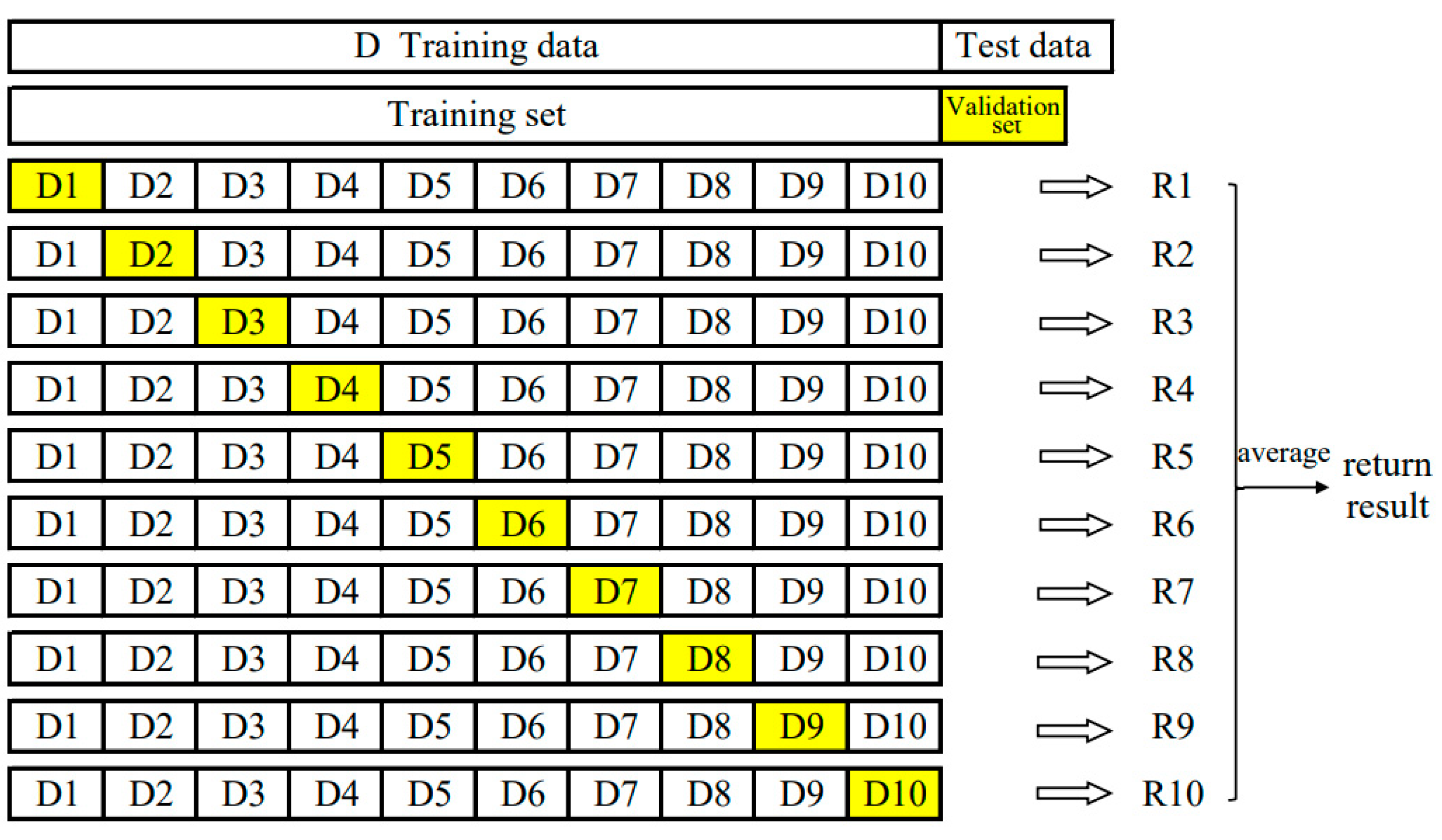
2.2.5. Model Hyperparameter Optimization

In this study, we combined K-fold cross-validation, grid search, and random search for hyperparameter optimization. Based on the 2-year period of water quality and sludge monitoring data, a 10-fold cross-validation method was used to tune the parameters of the ML models with hyperparameters to find the optimal hyperparameter values to improve the generalization performance (Figure 1). The data set was randomly divided into a training (80%) and testing (20%) set. Thus, the training and testing data sets in this study contained 584 and 147 data samples, respectively. The training set was divided into ten folds for parameter optimization, and each fold was used for training and validation in one iteration. The accuracy was evaluated using the coefficient of determination (R²). During the cross-validation process, the training iterations were set to 300.

2.2.6. Model Metrics

A variety of ML model metrics were used for the evaluation process, including root mean squared error (RMSE, m³/d), mean absolute error (MAE, m³/d), mean absolute percentage error (MAPE, p.u.), and decisive factor (R², p.u.):

$$RMSE=\sqrt{\frac{1}{m}{\displaystyle \sum _{i=1}^m{(f_i-y_i)}^2}},$$

(7)

$$MAE=\frac{1}{m}{\displaystyle \sum _{i=1}^m\left|f_i-y_i\right|},$$

(8)

$$MAPE=\frac{100\%}{m}{\displaystyle \sum _{i=1}^m\left|\frac{f_i-y_i}{y_i}\right|},$$

(9)

$$R^2=1-\frac{{\displaystyle \sum _{i=1}^m{(f_i-y_i)}^2}}{{\displaystyle \sum _{i=1}^m{({\overline{y}}_i-y_i)}^2}},$$

(10)

where m represents the total number of predictions, f is the predicted value, and y is the true value. An R² value closer to 1 indicates a greater correlation between the predicted and true values, indicating a better fit. For all the other metrics [Equations (7)–(10)], a smaller value indicates a smaller deviation and a better model performance. MAPE measures the accuracy of the model; RMSE evaluates the precision of the prediction and is sensitive to both extremely large and small errors in the result; and MAE measures the quality of the model prediction.

2.2.7. Modeling Process

Nine algorithms (as mentioned in Section 2.2.1) were used to predict sludge production from wastewater treatment. The main process included fusion and preprocessing of multi-source data, feature engineering (enhancement and filtering) of sample data, construction of ML models, and model evaluation and selection, described as follows:

• Data fusion and preprocessing: Fusion and preprocessing of multi-source data included time scale matching, deduplication, and filling/deleting missing values to form a sample set containing features and system response.
• Sample feature enhancement: The data set was normalized using Z-score normalization. Simultaneously, based on the sewage treatment process, we calculated the water quality concentration difference, reduction percentage, and indicator reduction amount before and after sewage treatment and added temperature and rainfall data under the corresponding time scale to achieve feature enhancement.
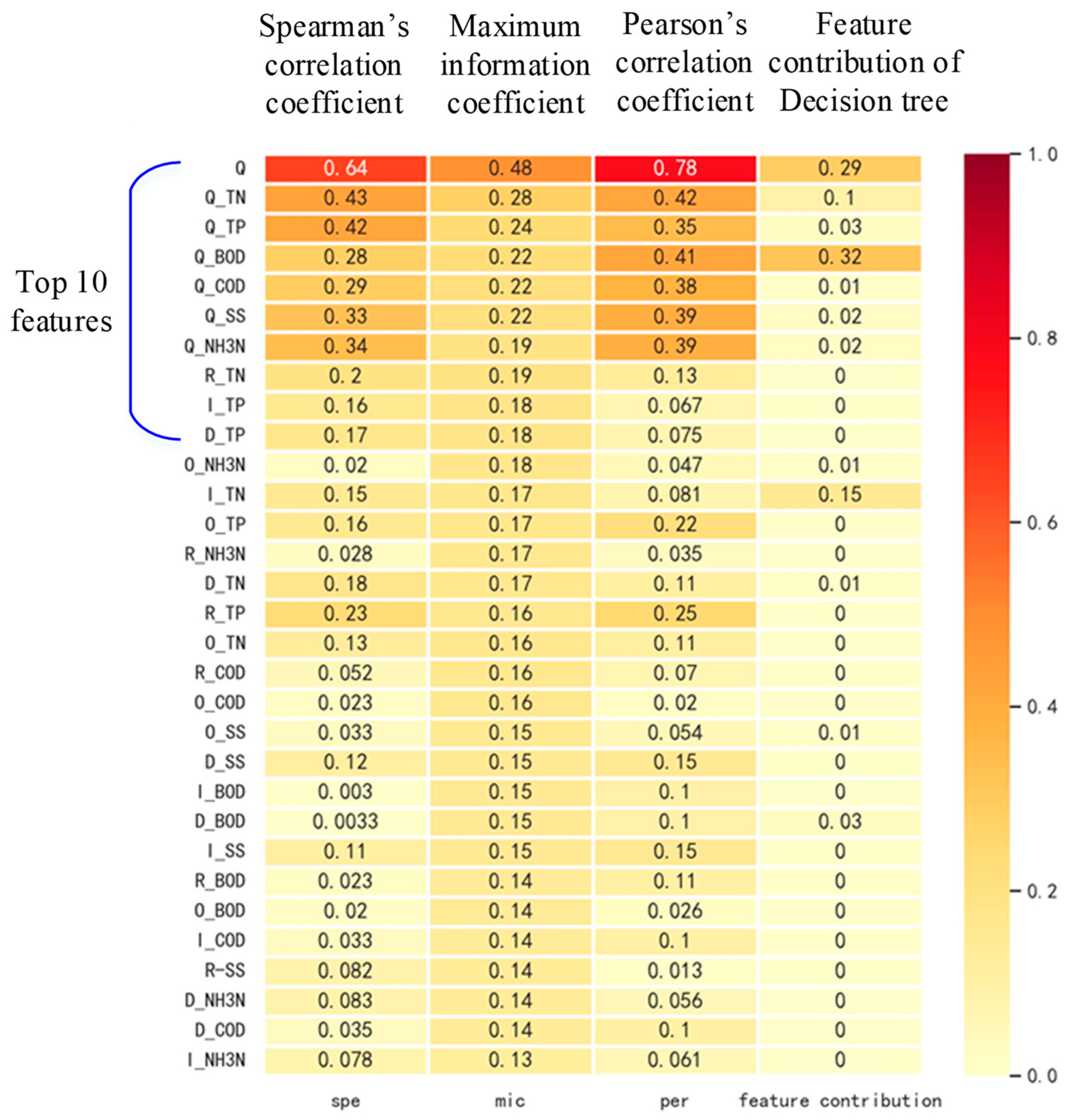
• Feature filtering: Multiple linear and nonlinear correlation analyses and feature contribution analyses were utilized to jointly filter out factors with lower sensitivity to the system response.
• ML model construction: All ML algorithms mentioned in Section 2.2.1 were combined with K-fold, grid search, and random search hyperparameter optimization to confirm the optimal structure for each type of model.
• Model evaluation and selection: MAP, RMSE, MAPE, and R² were used to evaluate the prediction performance of each model.

All the algorithms and analysis processes are implemented with the aid of the scikit-learn, XGBoost, minepy, and PyTorch libraries in Python 3.7, and a variety of standard packages such as pandas and Numpy are also utilized to perform the basic work of data processing.

3. Results and Discussion

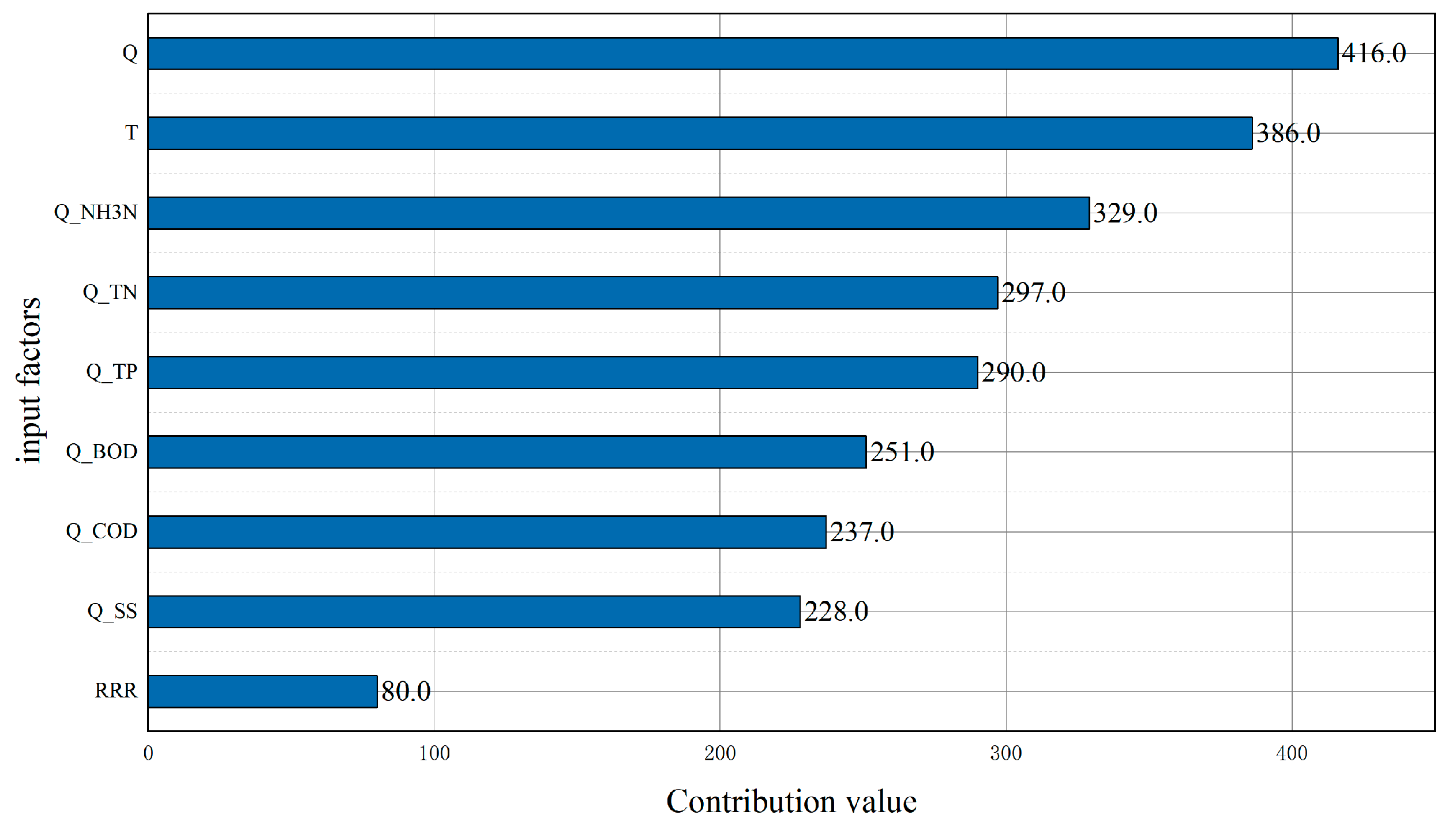
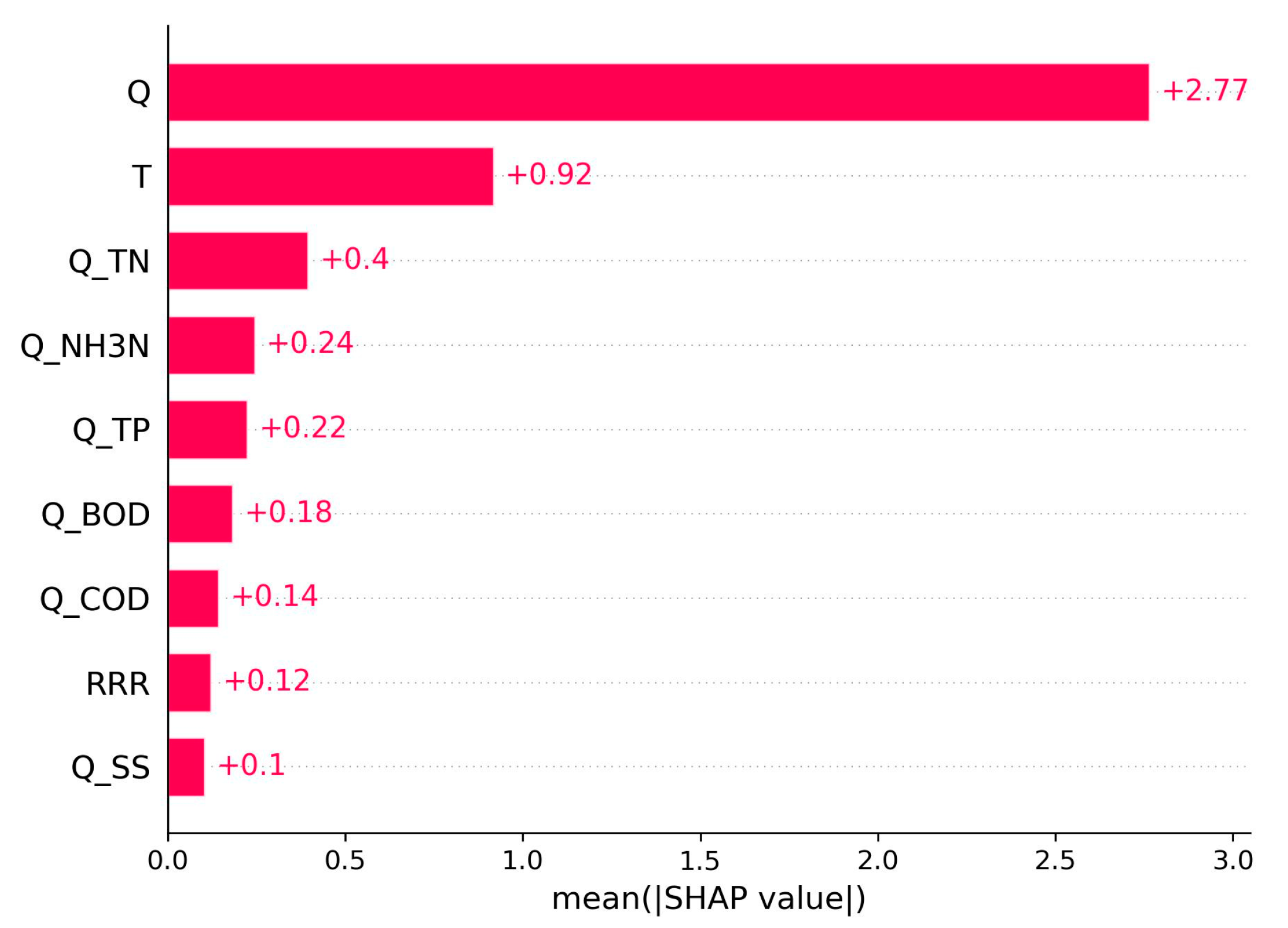
3.1. Feature Engineering Analysis

Figure 2 provided feature association results with the aid of the heatmap method. From Figure 2, it can be seen that the top 10 features from the four analyses all included the same water-quality indicators, such as water volume, TP removal, TN removal, BOD removal, COD removal, SS removal, and ammonia nitrogen removal. Out of these, the water-quality variables with the highest sensitivity to system response (sludge production amount) were obtained, and the feature-enhanced data set was filtered. At the same time, temperature and rainfall features are also considered, bringing about a total of 9 features to be used as inputs for the next stage of prediction modeling.

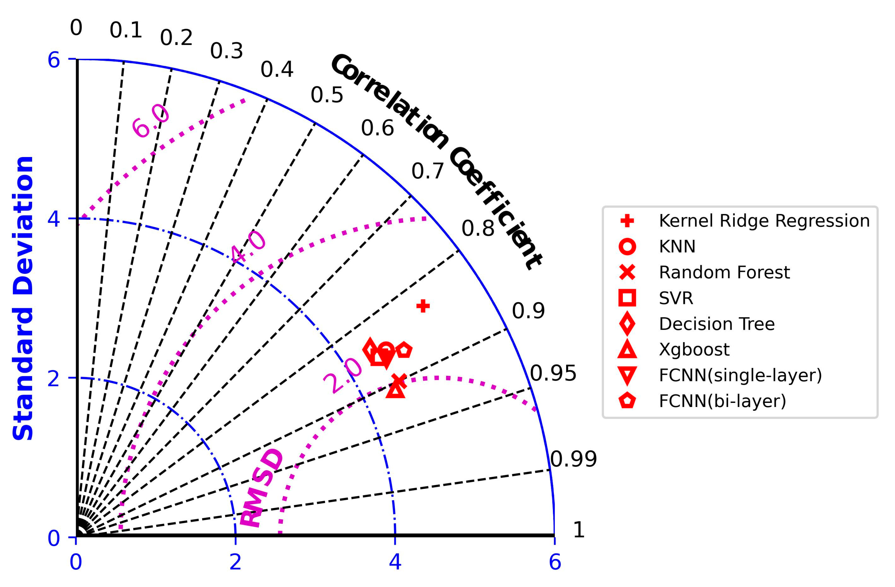
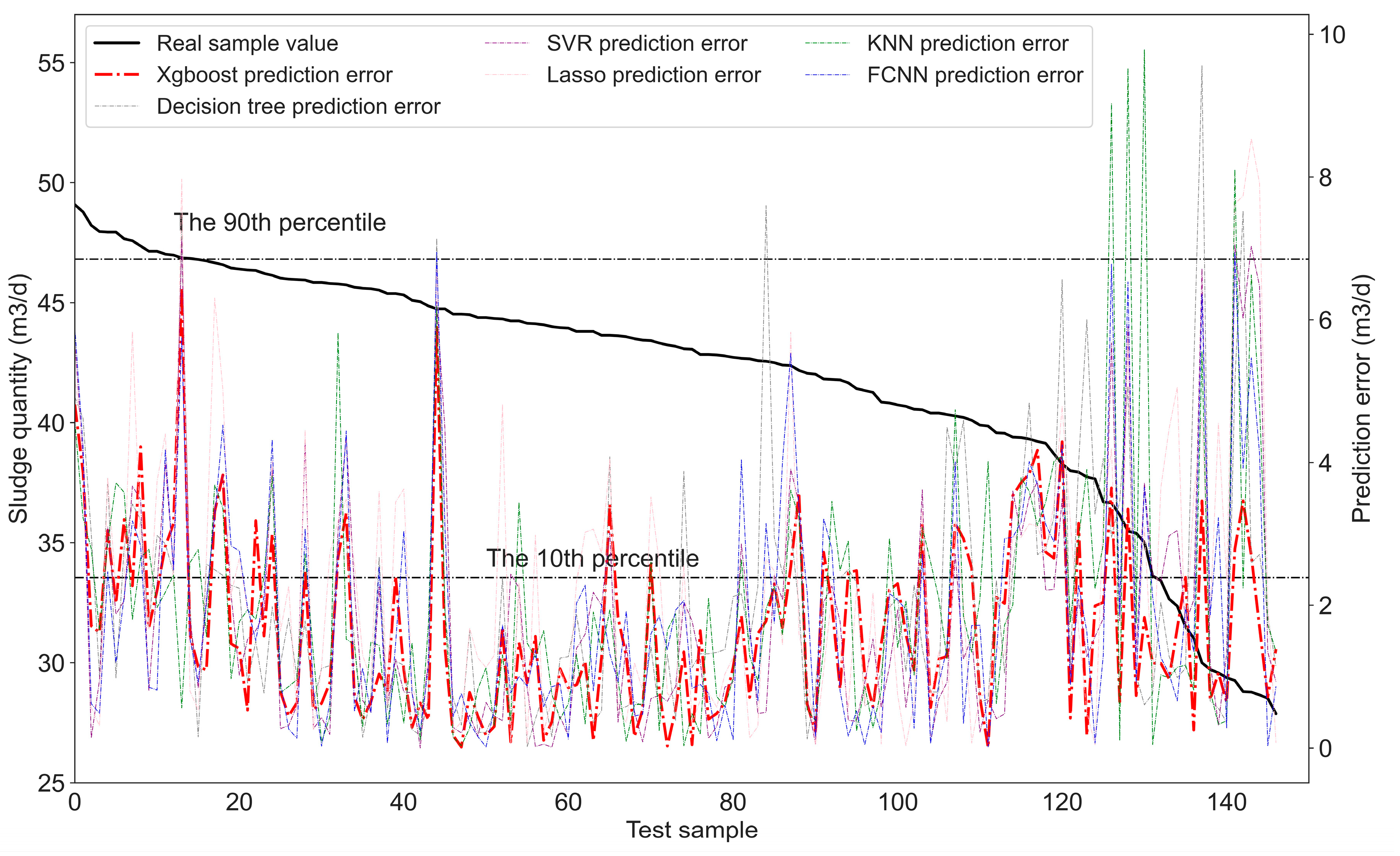
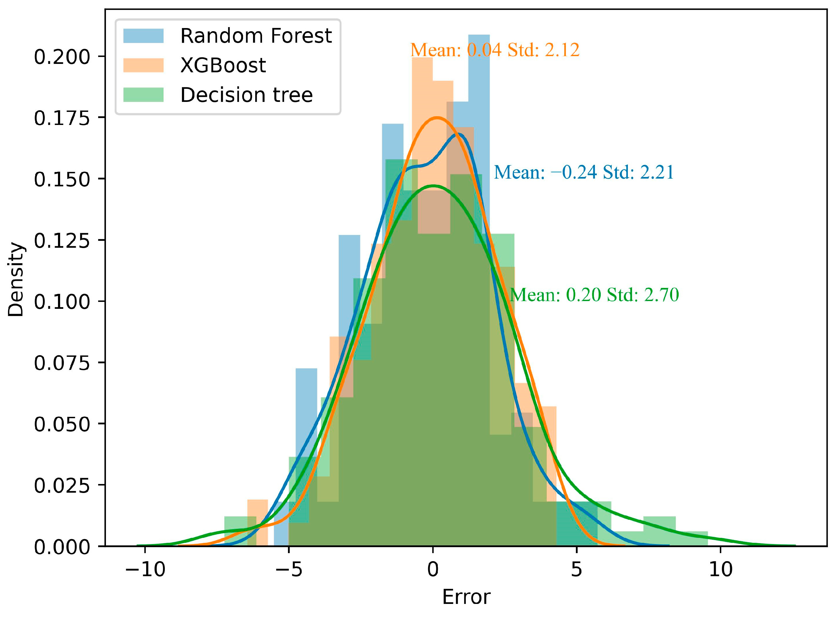
3.2. Optimal Result Analysis

After hyperparameter optimization based on the training set, the metrics for the sludge generation capacity predicted by each model showed significant variations (

Table 2. Performance evaluation of different ML/ensemble learning sludge production prediction models on the test data set.

Model	Factors Selected for Hyperparameter Optimization	RMSE (m3/d)	MAE (m3/d)	MAPE (p.u.)	R2 (p.u.)
Lasso Regression	alpha = 0.01	2.9891	2.1147	0.05149	0.6470
Kernel Ridge Regression	kernel = ‘polynomial’ alpha = 0.7333333 degree = 3	2.0723	2.7216	0.05112	0.7074
DT	max_features = 6 max_depth = 5	2.7085	2.0878	0.05201	0.7083
SVR	C = 1 gamma = 0.1 epsilon = 0.01	2.5850	1.9793	0.04809	0.7360
KNN Regression	n_neighbors = 9	2.6187	2.0260	0.04949	0.7291
FCNN (single-layer)	weight_decay = 0.005 momentum = 0.9 learning_rate = 0.01 epoch = 10,000 network structure = 1024	2.5198	1.9546	0.04743	0.7492
FCNN (bi-layer)	weight_decay = 0.005 momentum = 0.9 learning_rate = 0.01 epoch = 10,000 network structure = 1024 × 1024	2.2464	1.7707	0.04319	0.8006
RF	max_features = 7 max_depth = 7 n_estimators = 365	2.2090	1.7710	0.04297	0.8072
XGBoost	learning_rate = 0.1147 n_estimators = 90 max_depth = 5	2.1169	1.7032	0.0415	0.8218

). The RMSE, MAE, MAPE, and R² values were in the range of 2.1169–2.9891, 1.7032–2.7216, 0.0415–0.05201, and 0.6470–0.8218, respectively. Evaluating the variations of these values revealed poor prediction results for the lasso regression, kernel ridge regression, and DT models. For example, the MAPE value for the DT model was 0.05201, and the MAE value for the kernel ridge regression was 2.7216, the highest value in these categories. In comparison, the metrics for the ensemble learning model, XGBoost, were ranked significantly better than all the other models. Its RMSE, MAE, MAPE, and R² values were 2.1169, 1.7032, 0.0415, and 0.8218, respectively. Although RF, another ensemble learning model, was inferior to the XGBoost model, it still had a better predictive capability compared to the other models. Its RMSE, MAE, MAPE, and R² values were 2.2090, 1.7710, 0.04297, and 0.8072, respectively.

Therefore, compared to traditional ML algorithms such as SVR, DT, KNN regression, lasso, and kernel ridge regressions, ensemble learning algorithms had a clear advantage in prediction performance. Unlike FCNNs, ensemble learning was slightly superior to NNs. The RMSE, MAE, MAPE, and R² values for the bi-layer neural network with 1024 neurons per layer were 2.2464, 1.7707, 0.04319, and 0.8072, respectively, slightly poor compared to those of RF and XGBoost. Considering the factor of random noise, this has a minor impact on the practical application of wastewater treatment engineering and scientific research in the sludge field. However, by adding the analysis of the model complexity and computation time, the performance of the ensemble learning models based on DTs was significantly better than that of FCNN models. Specifically, the computation time, from the beginning to the end of the optimization training, for the FCNN and XGBoost models were 191.21 s and 123.50 s, i.e., the sludge prediction capability of XGBoost was faster by 35.41%. This effect was mainly because of the XGBoost model adopting a parallel computing method, reducing the overall computation time. By comparing the evaluation metrics individually for each model, the complex ensemble models were found to have a significantly higher ability to predict sludge production than the simpler basic ML models (or base learners), for example, RF/XGBoost vs. DT and bi-layer FCNN vs. single-layer FCNN.

Simultaneously, we provide Taylor diagrams (Figure 3) to visually compare model performances. Based on the Taylor diagrams, it is evident that the models of XGBoost and Random Forest perform well, with the XGBoost model exhibiting the best performance. It has the smallest root mean squared error (RMSE), a standard deviation closer to zero, and the highest correlation between predicted and actual values in the test dataset. On the other hand, other models, especially the Ridge Regression model, exhibit relatively poorer performance, indicated by higher RMSE, larger standard deviation, and lower correlation coefficient. Other models, such as Decision Tree, K-Nearest Neighbors (KNN), and Support Vector Regression (SVR), exhibit performance metrics between those of the XGBoost and Ridge Regression models. The diagram of performance by different ML/ensemble learning sludge production prediction models is presented in Figure 3.

Figure 4 shows the sludge production prediction for the DT and XGBoost models. The DT prediction ability was relatively general for the water quality–sludge sample set, with some samples having large prediction errors. In some cases, such as the 2530–4550 interval, multiple true values corresponded to the same prediction results. This effect was mainly determined by the DT features, i.e., by the division of features on each node and the corresponding division point. Similar test samples falling into a particular leaf node had the same predicted value (average of all training samples that fall in that node). In addition, the sludge prediction of the DT was prone to outliers. Ensemble learning models, i.e., RF and XGBoost, which use DTs as the base learners, can take advantage of the strengths of DTs and compensate for their limitations through the combination of bagging or boosting methods, thereby achieving a closer fit (smaller RMSE, and MAPE) or a more accurate restoration of the true sample situation (higher R²). The fitting effect of the XGBoost model on the sludge quantity was significantly better than that of the DT model. The predicted values were closer to the true value of the sample sludge production and were densely distributed on both sides of the regression line.

Generally, the model performance is often evaluated using model metrics such as RMSE, MAE, MAPE, and R². To further highlight the superiority of our chosen model (i.e., the XGBoost model), we analyzed the performance of each model on extreme samples in the test set (arranged in descending order) by using the absolute errors of predictions (Figure 5). From the dual-axis graph (where the left y-axis represents sludge quantity and the right y-axis represents absolute prediction errors), it could be seen that the XGBoost model performs well on extreme samples in the test set. In the case of extreme minimum value samples (such as the samples with sludge quantity below the 10th percentile, 33.54 m³/d), the XGBoost model exhibited lower absolute prediction errors compared to other models, with errors all below 4 m³/d. In the case of extreme maximum value samples (such as the samples with sludge quantity above the 90th percentile, 46.82 m³/d), the absolute prediction errors of the XGBoost model were all below 7 m³/d, still lower than most of the other models.

We also analyzed the prediction error distribution of the XGBoost, Random Forest, and Decision Tree models, as shown in Figure 6. It could be observed that the errors of the models showed approximately normal distribution, consistent with expectations. The mean errors of the models were all around 0, with XGBoost having the smallest bias while Random Forest had the largest bias. In terms of the standard deviation of model errors, XGBoost had the smallest variance, while Decision Tree exhibited the largest. These results further demonstrated the superior predictive performance of the XGBoost model chosen in this study.

Using the XGBoost model with the optimal prediction performance for sludge production, we further analyzed the contribution of each feature in the input model to the system response (sludge amount; Figure 7). The contributions were calculated using the weight method to measure their importance. This method counts the number of times each feature is called when the subtrees of all base learners (DTs) are split, and the final contribution ranking results are obtained through sorting.

Daily wastewater treatment volume feature had the greatest impact on the prediction results (Figure 7) as the magnitude of sludge production is directly related to the quantity of inflowing water. The temperature feature also had a strong influence as it affects the assimilation and dissimilation of microorganisms. The sludge decay coefficient increased with increasing temperature, leading to the reduction of the apparent sludge yield coefficient. On the other hand, factors such as seasonal variations and abnormal temperature changes directly caused fluctuations in sludge production. The influent contains various basic organic and inorganic substances needed to form sludge. According to the results, the various water quality indicators were ranked (from highest to lowest) according to their influence on sludge production, such as ammonia nitrogen, TN, TP, BOD₅, COD, and SS. The rainfall feature also had an impact as the wastewater treatment plant did not separate stormwater and wastewater, and the generation of sludge also included certain substances brought in by rainwater.

SHAP (SHapley Additive exPlanations) analysis is an important method for model interpretation. Through the SHAP values of attributes, the impact of each attribute on predictions can be explained, revealing the sensitivity of the model to attributes. We conducted a SHAP value analysis on the XGBoost model and obtained Figure 8. From the SHAP plot, it is evident that the attribute with the most significant impact is still the influent wastewater volume (Q), followed by environmental temperature (T). These results align with the input feature contributions of the XGBoost model itself. However, when comparing to Figure 7, it can be observed that the importance of Q_TN has increased in the SHAP analysis of water quality indicators, while the importance of Q_SS has decreased. This discrepancy is due to SHAP values focusing more on the contribution of each feature within each sample, while the model’s feature contribution reflects the feature’s weight (optimized through overall prediction bias), resulting in differing results between the two methods.

The comparison of evaluation results of the models with different complexities indicated that the lower the model complexity, the poorer the evaluation metrics for the test set. These metrics for the testing set were closer to those for the training set (i.e., the metrics in

Table 3. Performance evaluation of different ML/ensemble learning sludge production prediction models on the train data set.

Model	Factors Selected for Hyperparameter Optimization	RMSE (m3/d)	MAE (m3/d)	MAPE (p.u.)	R2 (p.u.)
Lasso Regression	alpha = 0.01	2.7901	2.1218	0.05324	0.6875
Kernel Ridge Regression	kernel = ‘polynomial’ alpha = 0.7333333 degree = 3	2.5106	1.9268	0.04780	0.7470
DT	max_features = 6 max_depth = 5	2.0847	1.6389	0.0393	0.8255
SVR	C = 1 gamma = 0.1 epsilon = 0.01	2.3173	1.6148	0.04026	0.7841
KNN Regression	n_neighbors = 9	2.4501	1.8520	0.04572	0.7590
FCNN (single-layer)	weight_decay = 0.005 momentum = 0.9 learning_rate = 0.01 epoch = 10,000 network structure = 1024	1.9060	1.4605	0.03602	0.8539
FCNN (bi-layer)	weight_decay = 0.005 momentum = 0.9 learning_rate = 0.01 epoch = 10,000 network structure = 1024 × 1024	1.7695	1.3694	0.03342	0.8743
RF	max_features = 7 max_depth = 7 n_estimators = 365	1.2015	1.4862	0.02905	0.9112
XGBoost	learning_rate = 0.1147 n_estimators = 90 max_depth = 5	1.1723	1.4925	0.02852	0.9106

), reflecting that the models with a lower complexity had a lower variance in prediction results and a larger bias. On the contrary, the models with a higher complexity had a larger discrepancy between the test and training set evaluation metrics, suggesting that models with a higher complexity had a higher variance in prediction results and a smaller bias.

More specifically, the XGBoost model will also have better prediction ability than the RF model with a fast learning speed and high accuracy from previous literature [7]. XGBoost is an ensemble learning algorithm based on decision trees. It generates multiple weak learners through continuous iteration; each weak learner fits on the previous weak learner’s prediction error, and finally, the leaf values on all weak estimators are weighted and summed directly to get the final prediction result. Compared with the XGBoost model, RF selects features and samples randomly to build each decision tree, and the generated multiple decision trees are averaged or voted to get the final prediction result. The XGBoost model has faster training and prediction speed than RF and can fine-adjust hyper-parameters to get better prediction results.

4. Conclusions

This study innovatively combined various data-driven techniques to realize the effective prediction of sludge production using water quality and volume, temperature, and rainfall data through data fusion, feature enhancement and filtering, and model screening.

The comparison of metrics for the different categories of ML and ensemble learning models shows that the prediction effect of the XGBoost model is better than that of the others. Its RMSE, MAE, MAPE, and R² values are 4.4815, 2.1169, 1.7032, 0.0415, and 0.8218, respectively. The RF model prediction performance is second only to the XGBoost model, reflecting the superiority of ensemble learning in fitting highly nonlinear data. The traditional base learners, such as DTs, lasso regression, and kernel ridge regression, have mediocre predictive performances for sludge production. On the other hand, more complex models, such as FCNNs, have a large number of parameters, which also leads to longer training times. Compared to XGBoost and RFs, NNs are not cost-effective, even though their prediction accuracies are quite similar. Therefore, we can infer that the relatively complex ensemble learning models have a superior prediction accuracy compared to the traditional base learners, especially on small and medium-scale datasets. Furthermore, compared to other high-complexity models, such as FCNNs, ensemble learning models have a superior computational efficiency.

By analyzing the importance of each input model feature to system response (sludge volume), the effectiveness of feature engineering using complex correlation techniques (Pearson’s correlation coefficient, Spearman’s correlation coefficient, and maximum information coefficient correlation analyses) was verified. Simultaneously, the selected XGBoost model also provided the contribution ranking of each feature. The daily wastewater treatment volume and temperature features had the greatest impact on sludge production. This analysis further verifies the feasibility, interpretability, and efficiency of using high-complexity models on small- and medium-sized samples.

References

1. Ministry of Housing and Urban-Rural Development of the People’s Republic of China. 2021 China Urban-Rural Construction Statistical Yearbook. Available online: https://www.mohurd.gov.cn/gongkai/fdzdgknr/sjfb/index.html (accessed on 30 May 2023).
2. Wang, L. Analysis of seasonal variation and influencing factors of sludge yield in municipal sewage plant. Water Purif. Technol. 2018, 37, 36–40. [Google Scholar]
3. Ministry of Ecology and Environment of the People’s Republic of China. Technical Specification for Application and Issuance of Pollutant Permit-Wastewater Treatment (on Trial). [EB/OL]. Available online: https://www.mee.gov.cn/ywgz/fgbz/bz/bzwb/pwxk/201811/t20181115_673874.shtml (accessed on 31 May 2023).
4. Henze, M.; Grady, C., Jr.; Gujer, W.; Matsuo, T. Activated Sludge Model No.1: IWA Scientific and Technical Report No.1; IAWPRC: London, UK, 1987. [Google Scholar]
5. Zhou, B.; Zhou, D.; Zhang, L.W.; Yu, F.H. Discussion on the design calculation method of activated sludge process. China Water Wastewater 2001, 17, 45–49. [Google Scholar]
6. GB50014-2021; Standard for Design of Outdoor Wastewater Engineering. China Planning Press: Beijing, China, 2021.
7. Jian, P.; Han, H.S.; Yi, Y.; Huang, H.; Xie, L. Machine learning and deep learning modeling and simulation for predicting PM2.5 concentrations. Chemosphere 2022, 308, 136353. [Google Scholar]
8. Quintelas, C.; Melo, A.; Costa, M.; Mesquita, D.; Ferreira, E.; Amaral, A. Environmentally-friendly technology for rapid identification and quantification of emerging pollutants from wastewater using infrared spectroscopy. Environ. Toxicol. Phar. 2020, 80, 103458. [Google Scholar] [CrossRef] [PubMed]
9. Torregrossa, D.; Leopold, U.; Hernández-Sancho, F.; Hansen, J. Machine learning for energy cost modelling in wastewater treatment plants. J. Environ. Manag. 2018, 223, 1061–1067. [Google Scholar] [CrossRef]
10. Vyas, M.; Kulshrestha, M. Artificial neural networks for forecasting wastewater parameters of a common effluent treatment plant. Int. J. Environ. Waste Manag. 2019, 24, 313–336. [Google Scholar] [CrossRef]
11. Ozkan, O.; Ozdemir, O.; Azgin, T.S. Prediction of Biochemical Oxygen Demand in a Wastewater Treatment Plant by Artificial Neural Networks. Chem. Asian. J. 2009, 21, 4821–4830. [Google Scholar]
12. Dong, W.; Sven, T.; Ulrika, L.; Jiang, L.; Trygg, J.; Tysklind, M.; Souihi, N. A machine learning framework to improve effluent quality control in wastewater treatment plants. Sci. Total. Environ. 2021, 784, 147138. [Google Scholar]
13. Zhou, P.; Li, Z.; Snowling, S.; Baetz, B.W.; Na, D.; Boyd, G. A random forest model for inflow prediction at wastewater treatment plants. Stoch Environ. Res. Risk Assess. 2019, 33, 1781–1792. [Google Scholar] [CrossRef]
14. Liu, Z.-J.; Wan, J.-Q.; Ma, Y.-W.; Wang, Y. Online prediction of effluent COD in the anaerobic wastewater treatment system based on PCA-LSSVM algorithm. Evnviron. Sci. Pollution Res. 2019, 26, 12828–12841. [Google Scholar] [CrossRef]
15. Wang, R.; Yu, Y.; Chen, Y.; Pan, Z.; Li, X.; Tan, Z.; Zhang, J. Model construction and application for effluent prediction in wastewater treatment plant: Data processing method optimization and process parameters integration. J. Environ. Manag. 2022, 302, 114020. [Google Scholar] [CrossRef] [PubMed]
16. Bagherzadeh, F.; Mehrani, M.-J.; Basirifard, M.; Roostaei, J. Comparative study on total nitrogen prediction in wastewater treatment plant and effect of various feature selection methods on machine learning algorithms performance. J. Water Process Eng. 2021, 41, 102033. [Google Scholar] [CrossRef]
17. Miao, S.; Zhou, C.; AlQahtani, S.A.; Alrashoud, M.; Ghoneim, A.; Lv, Z. Applying machine learning in intelligent sewage treatment: A case study of chemical plant in sustainable cities. Sustain. Cities Soc. 2021, 702, 103009. [Google Scholar] [CrossRef]
18. Mehrani, M.-J.; Bagherzadeh, F.; Zheng, M.; Kowal, P.; Sobotka, D.; Mąkinia, J. Application of a hybrid mechanistic/machine learning model for prediction of nitrous oxide (N2O) production in a nitrifying sequencing batch reactor. Process Saf. Environ. 2022, 162, 1015–1024. [Google Scholar] [CrossRef]
19. Wu, X.; Zheng, Z.; Wang, L.; Li, X.; Yang, X.; He, J. Coupling process-based modeling with machine learning for long-term simulation of wastewater treatment plant operations. J. Environ. Manag. 2023, 341, 118116. [Google Scholar] [CrossRef] [PubMed]
20. Arslan, K.; Imtiaz, A.; Wasif, F.; Naqvi, S.R.; Mehran, M.T.; Shahid, A.; Liaquat, R.; Anjum, M.W.; Naqvi, M. Investigation of combustion performance of tannery sewage sludge using thermokinetic analysis and prediction by artificial neural network. Case Stud. Therm. Eng. 2022, 40, 102586. [Google Scholar]
21. Usman, S.; Jorge, L.; Hai-Tra, N.; Yoo, C. A hybrid extreme learning machine and deep belief network framework for sludge bulking monitoring in a dynamic wastewater treatment process. J. Water Process Eng. 2022, 46, 102580. [Google Scholar]
22. Bi, H.; Wang, C.; Jiang, X.; Jiang, C.; Bao, L.; Lin, Q. Thermodynamics, kinetics, gas emissions and artificial neural network modeling of co-pyrolysis of sewage sludge and peanut shell. Fuel 2021, 284, 118988. [Google Scholar] [CrossRef]
23. Flores-Alsina, X.; Ramin, E.; Ikumi, D.; Harding, T.; Batstone, D.; Brouckaert, C.; Sotemann, S.; Gernaey, K.V. Assessment of sludge management strategies in wastewater treatment systems using a plant-wide approach. Water Res. 2021, 190, 116714. [Google Scholar] [CrossRef]
24. Xu, Z. Study on influencing factors of initial sludge yield in municipal sewage treatment. Urban Roads Bridges Flood Control. 2014, 3, 80–82. [Google Scholar]
25. Wu, H.M. A Study on Sludge Production in City Sewage Treatment Works. China Munic. Eng. 1998, 83, 40–42. [Google Scholar]
26. Ministry of Ecology and Environment of the People’s Republic of China. Discharge Standard of Pollutants for Municipal Wastewater Treatment Plant (GB 18918-2002). [EB/OL]. Available online: https://www.mee.gov.cn/ywgz/fgbz/bz/bzwb/shjbh/swrwpfbz/200307/t20030701_66529.shtml (accessed on 1 June 2023).
27. China Urban Water Association. Annual Report of Chinese Uran Water Utilities (2019); China Architecture & Building Press: Beijing, China, 2020; pp. 130–140. [Google Scholar]
28. State Environmental Protection Administration of China. Water and Wastewater Monitoring and Analysis Methods, 4th ed.; China Environmental Science Press: Beijing, China, 2002; pp. 210–213. [Google Scholar]
29. Robert, T. Regression shrinkage and selection via the lasso. J. R. Statist. Soc. 1996, 58, 267–288. [Google Scholar]
30. Miller, A. Subset Selection in Regression, 2nd ed.; Chapman & Hall/CRC: New York, NJ, USA, 2002. [Google Scholar]
31. Draper, N.R.; Smith, H. Applied Regression Analysis, 3rd ed.; Wiley: Hoboken, NJ, USA, 1998. [Google Scholar]
32. Hunt, E.B.; Marin, J.; Stone, P.J. Experiments in induction. Acad. Press 1966, 80. [Google Scholar]
33. Vapnik, V. The Nature of Statistical Learning Theory; Springer: New York, NY, USA, 1999. [Google Scholar]
34. Denoeux, T. A k-nearest neighbor classification rule-based on dempster-shafer theory. IEEE Trans. Syst. Man Cybern. 1995, 25, 804–813. [Google Scholar] [CrossRef]
35. Breiman, L. Random forests. Mach. Learn. 2001, 45, 5–32. [Google Scholar] [CrossRef]
36. Chen, T.Q.; Guestrin, C. Xgboost: A Scalable Tree Boosting System. In Proceedings of the 22nd ACM SIGKDD International Conference on Knowledge Discovery and Data Mining, San Francisco, CA, USA, 13–17 August 2016; pp. 785–794. [Google Scholar]
37. Pearson, K. Notes on regression and inheritance in the case of two parents. Proc. R. Soc. Lond. 1895, 58, 240–242. [Google Scholar]
38. Fieller, E.C.; Hartley, H.O.; Pearson, E.S. Tests for rank correlation coefficients I. Biometrika 1957, 44, 470–481. [Google Scholar] [CrossRef]
39. Reshef, D.N.; Reshef, Y.A.; Finucane, H.K.; Grossman, S.R.; McVean, G.; Turnbaugh, P.J.; Lander, E.S.; Mitzenmacher, M.; Sabeti, P.C. Detecting novel associations in large data sets. Science 2011, 334, 1518–1524. [Google Scholar] [CrossRef] [PubMed]
Figure 1. Schematic representation of the ten-fold cross-validation method.
Sustainability 15 13380 g001
Figure 2. Feature association results heatmap.
Sustainability 15 13380 g002
Figure 3. Taylor diagram of performance by different ML/ensemble learning sludge production prediction models.
Sustainability 15 13380 g003
Figure 4. Comparison of the true sludge production values and values predicted by (a) DT and (b) XGBoost; Correlation between the predicted and true values of (c) DT and (d) XGBoost.
Sustainability 15 13380 g004
Figure 5. Comparison of different methods for test sample value in descending order.
Sustainability 15 13380 g005
Figure 6. Histogram of error distribution between actual and predicted values.
Sustainability 15 13380 g006
Figure 7. Input feature contributions for sludge production prediction using XGBoost. (Note: Q for Wastewater Quantity, T for Temperature, NH3N for Ammonia Nitrogen, RRR for Rainfall).
Sustainability 15 13380 g007
Figure 8. Input feature importance for sludge production prediction using XGBoost.
Sustainability 15 13380 g008