Sustainable Financial Fraud Detection Using Garra Rufa Fish Optimization Algorithm with Ensemble Deep Learning

Abstract

Sustainable financial fraud detection (FD) comprises the use of sustainable and ethical practices in the detection of fraudulent activities in the financial sector. Credit card fraud (CCF) has dramatically increased with the advances in communication technology and e-commerce systems. Recently, deep learning (DL) and machine learning (ML) algorithms have been employed in CCF detection due to their features’ capability of building a powerful tool to find fraudulent transactions. With this motivation, this article focuses on designing an intelligent credit card fraud detection and classification system using the Garra Rufa Fish optimization algorithm with an ensemble-learning (CCFDC-GRFOEL) model. The CCFDC-GRFOEL model determines the presence of fraudulent and non-fraudulent credit card transactions via feature subset selection and an ensemble-learning process. To achieve this, the presented CCFDC-GRFOEL method derives a new GRFO-based feature subset selection (GRFO-FSS) approach for selecting a set of features. An ensemble-learning process, comprising an extreme learning machine (ELM), bidirectional long short-term memory (BiLSTM), and autoencoder (AE), is used for the detection of fraud transactions. Finally, the pelican optimization algorithm (POA) is used for parameter tuning of the three classifiers. The design of the GRFO-based feature selection and POA-based hyperparameter tuning of the ensemble models demonstrates the novelty of the work. The simulation results of the CCFDC-GRFOEL technique are tested on the credit card transaction dataset from the Kaggle repository and the results demonstrate the superiority of the CCFDC-GRFOEL technique over other existing approaches.

1. Introduction

Financial fraud can be considered as any criminal activity related to payment processes, or any fraud targeting financial institutions such as banks, lending institutions, crypto exchanges, and fintechs. Financial fraud detection refers to protocols set in place to avoid the damage caused by fraudulent activities taking place within financial service providers. This can include credit card fraud, money laundering, identity theft, and other forms of payment fraud [1]. Credit card fraud is one of the easier varieties. Without any risk or the knowledge of the user, a considerable amount of money can be withdrawn in a small amount of time [2]. The fraudster operates by trying to make each successive transaction valid, and detecting this can be a very complex and challenging task [3]. A credit card is vulnerable to cybercrime, leading to credit card fraud. The fraudster performs fraudulent activity by gaining unauthorized access to credit card data and this activity causes a financial loss for the customer and company. Therefore, the challenges of fraudulent activity increase the demand for systems to identify credit card fraud (CCF) [4]. Research workers are attempting to construct fraud detection systems through data mining (DM), deep learning (DL), and machine learning (ML) methodologies to identify either whether the transaction is genuine or fraudulent, based on a dataset that includes transaction details. However, CCF detection (CCFD) becomes challenging because fraudulent transactions on a card can appear more and more like authorized ones [5]. To resolve these issues, credit card providers should apply increasingly complex techniques to identify fraudulent transactions. The most important problem is the lack of datasets. The datasets available for these problems have many unknown fields for private insurance and are imbalanced, making it hard for the programmer to understand them and to construct a better model that resolves these challenges [6].

With the enormous capacity of credit card transactions, automatically authenticating each transaction to identify fraud becomes impracticable for the credit card issuer [7]. As a result, statistical learning or ML techniques are most frequently used to automatically identify fraudulent transactions. There exists a great deal of positive feedback based on the ML technique in fraudulent recognition [8]. For supervised learning, prior studies mainly inspected statistical models with shallow architecture, for instance, hidden Markov chains, neural networks (NN), support vector machines (SVM), logistic regression (LR), and models with one hidden layer (HL). The shallow architecture model has single layer of non-linear conversion [9]. The non-linear conversion maps the raw input dataset from its original space into the feature space. As a natural extension to the shallow architecture model, the deep architecture model, called the DL algorithm, applies more than one layer of non-linear alteration and stacks those non-linear conversion layers in threes in a hierarchical model from which the output of the lower layer was processed as an input to the second layer. Recently, a deep architecture model has been reported to outperform conventional ML techniques for representation learning and pattern recognition in different fields involving image and speech coding, information retrieval, and image and speech recognition [10]. Thus, there was some discussion about whether DL is being effectively used for fraudulent detection.

This article focuses on the design of an intelligent credit card fraud detection and classification using the Garra Rufa Fish optimization algorithm with an ensemble-learning (CCFDC-GRFOEL) model. The CCFDC-GRFOEL model performs a Z-score data normalization process to convert the input dataset into a uniform format. Next, the CCFDC-GRFOEL method derives a new GRFO-based feature subset selection (GRFO-FSS) approach for selecting a set of features. The ensemble-learning process, comprising an extreme learning machine (ELM), bidirectional long short-term memory (BiLSTM), and autoencoder (AE) with pelican optimization algorithm (POA), is used for the detection of fraudulent transactions. The simulation results of the CCFDC-GRFOEL technique are tested on a credit card transaction dataset from the Kaggle repository.

The rest of the paper is organized as follows. Section 2 provides the related works and Section 3 offers the proposed model. Then, Section 4 gives the results analysis and Section 5 concludes the paper.

2. Related Works

Prabhakaran and Nedunchelian [11] introduced an Oppositional-Cat-Swarm-Optimization-based aspect selection procedure with a DL method for CCFD, abbreviated as the OCSODL-CCFD method. In this study, the Chaotic Krill Herd Algorithm (CKHA) and Bi-directional Gated Recurrent Unit (BiGRU) method were adapted for the categorization of CCF. The hyperparameters of the BiGRU method were fine-tuned with the implementation of the CKHA method. In [12], the authors primarily concentrated on processing the unbalanced records by employing an under-sampling method to acquire high accuracy, precision, and better outcomes through diverse ML procedures. The authors suggested an agenda based on combining the databases and by implementing the fuzzy C-means algorithm to choose the relevant fraud and standard illustrations with similar aspects that promise veracity amongst the data aspects. The authors of [13] proposed three innovative contributions. The first improvement was a data-balanced Deep Stacking Autoencoder (DSA) for FD that functions on the basis of the Harris Grey Wolf (HGW) network. In this study, the HGW network was suggested as a means to educate the DSA. The proposed HGW-based DSA was found to be the most efficient procedure in recognizing fraudulent activities by enforcing a fitness method. This fitness method practices to generate a few mistakes and calculates the maximum resolution over a series of repetitions.

Ileberi et al. [14] proposed an ML-based CCF identification engine, using the Genetic Algorithm (GA) method in order to select the aspect. After the selection of maximized factors, the suggested method employed the subsequent ML categorizers: Decision Tree (DT), LR, Naive Bayes (NB), Artificial Neural Network (ANN), and Random Forest (RF). Kajal and Kaur [15] conducted a study to identify the CCF transmissions via ML methods like NB and DT. The aim of the study was to provide a balance over the database with a Near-Miss under-sampling procedure. For the purpose of Feature Selection (FS), the data gain procedure was enforced. In [16], an innovative procedure called SVM, with Information Gain (SVMIG), was suggested to enhance the precision of detecting fraudulent communications with a huge true positive frequency. The model was proposed to identify the fraudulent activities in credit cards. In this work, a min–max normalization approach was implemented to regulate the characteristics, whereas the aspect set of the characteristics was minimized by implementing the data-gain-based character selection process. In [17], the authors suggested a novel structure for CCF identification based on the chronological modeling of records and by implementing an Attention Module (AM) and an LSTM Deep Recurrent Neural Network (DRNN). Specifically, the vigorousness of our proposed method is based on its bringing together the strengths of three sub-procedures, which are Uniform Manifold Approximation and Projection (UMAP), to select the major beneficial prediction aspects; LSTM networks, for the integration of transmission orders; and an AM to improve the LSTM accomplishments.

The authors of [18] developed a set of ML models such as Logistic Regression, decision tree, XGBoost, Naive Bayes, and Random Forest to detect credit card fraud. Devi et al. [19] introduced a novel, fully connected neural network system in combination with oversampling of the classes to detect fraud. The deep, fully connected neural network was developed while the actual dataset was fitted to extract the fraud class. In this study, the class distribution was investigated and validated on imbalanced target data distribution. In [20], a novel Unsupervised-Attentional-Anomaly-Detection-Network-based CCF classification model (UAAD-FDNet) was introduced. Various transactions occur in a day while fraudulent transactions among them are considered as abnormal instances. In this scenario, autoencoders with Feature Attention and GANs can be employed as part of the effective classification of huge volumes of transaction data. In [21], the authors offered an ML model for the prediction of user click fraud. The model helps in differentiating the fraudulent and legitimate clicks, thereby finding the fraudulent users among the legitimate ones. The authors of [22] employed two unpublished datasets that might unravel novel knowledge, and four machine learning methods, including Support Vector Machines (SVM), Decision Trees (DT), Random Forest (RF), and Multilayer Perceptron (MLP) to determine the ML models used for the detection of medical fraud.

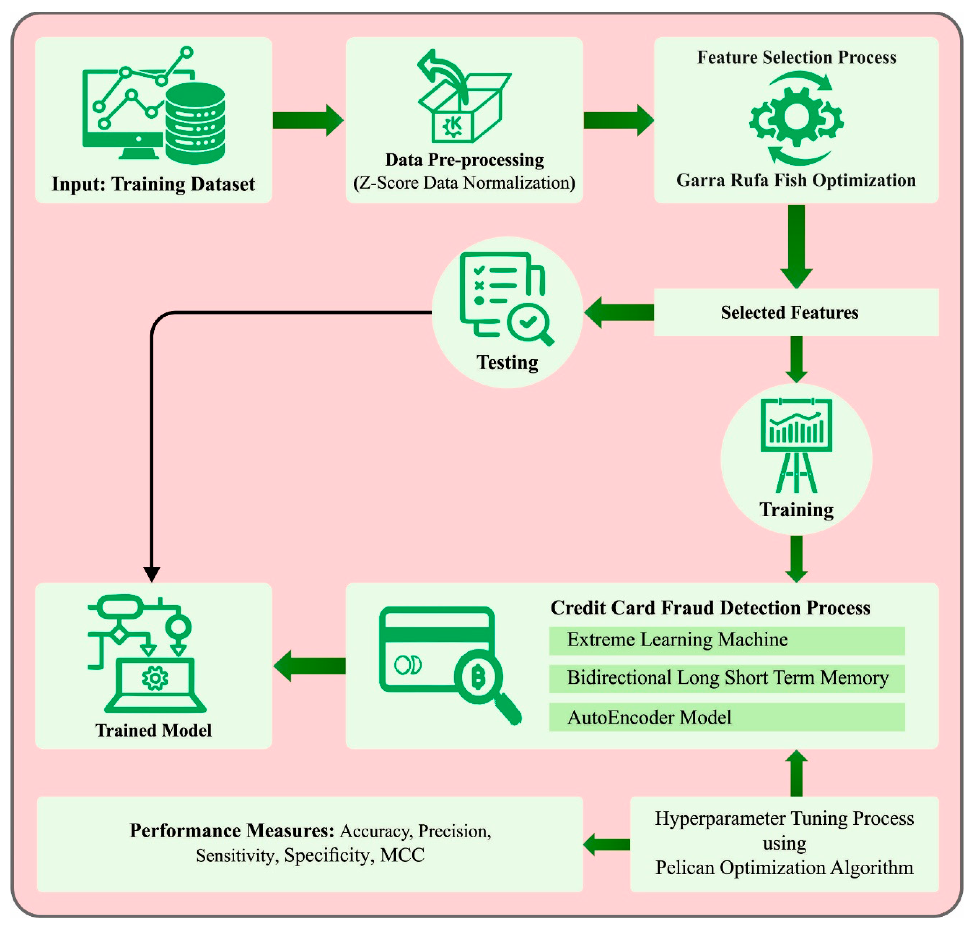
3. The Proposed Model

In this study, a new CCFDC-GRFOEL method has been introduced for both detection and classification of credit card fraud. The presented CCFDC-GRFOEL technique follows a three-stage process involving Z-score normalization, GRFO-based feature subset selection, ensemble-learning classification, and POA-based parameter tuning. Figure 1 illustrates the overall flow of the proposed CCFDC-GRFOEL method.

3.1. Data Normalization

During the primary stage, the Z-score normalization process is applied to measure the input dataset for which the formula is shown in Equation (1):

$$X_{stand}=\frac{X-mean \left(X\right)}{Standard Deviation \left(X\right)}$$

(1)

This Z-score normalization approach is highly effective for several optimization methods, namely Gradient Descent (GD), and is being increasingly applied in ML techniques.

3.2. Feature Selection Using GRFO Algorithm

In order to improve the classification results, the CCFDC-GRFOEL approach applies the GRFO-FSS approach for the selection of a set of features. GRFO is a new optimization technique, proposed on the basis of the distinctive movement of Garra Rufa fish, envisioned as moving between a submerged pair of legs, through ‘fish rubbing assembly’ [23]. Here, the particles are divided into groups, among which the best one is identified from each of the groups. Some of these particles are allowed to adjust the group, according to the fitness of their group leader. The mobility among those groups is determined by the amount of fish in all the groups. The fish are arranged in distinct groups and when finding their food, all the groups have their way to find the operational point of the system. All the groups are combined with their leader, and a similar amount of particles, which are called followers. According to the value, the followers change their group during each iteration. In the presented work, the GRFO technique is exploited to evaluate the reference that exists in the integrated PV-PEV technique. The working process of the GRFO technique is as follows

Step 1:

Initialization

In this phase, the voltage values, currents, and load demands are initialized.

Step 2:

Random generation

The initialized parameter is generated in an arbitrary fashion by the matrix.

Step 3:

Fitness calculation

Based on the objectives of the system, fitness computation is performed as given below.

$$F_i=\mathrm{M}\mathrm{i}\mathrm{n}\left(e\right),$$

(2)

Here, $e$ denotes the error function and it restores the system parameter, according to the Fitness Function (FF).

Step 4:

Resort the parameter

According to the FF, the parameters of the system are resorted.

Step 5:

Check the iteration

Check whether the maximal iteration and the optimum reference values are attained.

The number of leaders, used for the selection process, increases the complexity of the problem whereas the expected number has an optimum point for the objective method. Every time, a specific group of fish travels from one group to the other, it is better to pay the optimum fare between the enabled groups. If not, then the maximal iterations are accomplished and then return to the following steps.

Step 6:

Upgrade the parameter

Upgrade the amount of particles for all the groups as defined below.

$$N_f=\frac{n-N_L}{N_L},$$

(3)

In Equation (3), $n$ denotes the overall number of particles, $N_f$ shows the number of represented followers, and $N_L$ indicates the number of leaders.

Step 7:

Find the best and the worst leaders

The worst leader is defined as follows.

$$N_f=int(\alpha \times rand),$$

(4)

$$m_{ij}=\mathrm{m}\mathrm{a}\mathrm{x}\left(\left(m_{ij-1}-N_f\right), 0\right),$$

(5)

Now, $M_{ij}$ denotes the mobile fish for the $i$-$th$ leader. The best leader is defined as follows.

$$N_1=\sum _2^n{N}_i,$$

(6)

$$m_{1j}=m_{1_d-1}+N_1.$$

(7)

Step 8:

Upgrade the position as well as the speed

Both location and velocity are defined using the following expressions.

$$v_i(t+1)=\omega v_i\left(t\right)+c_1{R}_1\left(p_i\right(t)-X_i(t\left)\right)+c_2{R}_2\left(g_i\left(t\right)-X_i\left(t\right)\right),$$

(8)

$$X_i\left(t+1\right)=X_i\left(t\right)+v_i\left(t+1\right),$$

(9)

In these expressions, $V_i$ denotes the speed of the $i$-$th$ atom, $\omega$ represents the inactivity mass parameter, and $C_1,$ and $C_2$ indicate the acceleration coefficients. After updating the equations, the loop is interconnected to Step 3.

The FF considers the number of selected features as well as the classifier’s accuracy. It minimizes the set size of the selective features and maximizes the classification accuracy. Thus, the FF is used to assess the individual solution as given below.

$$Fitness=\alpha \ast ErrorRate+\left(1-\alpha \right)\ast \frac{\#SF}{\#All\_F}$$

(10)

Now, $ErrorRate$ indicates the classifier’s error rate.$ErrorRate$ is calculated as a percentage of improper classifications to the whole classifications made and is indicated as a value within [$\mathrm{0,1}$], $\#SF$ denotes the chosen features and $\#All\_F$ denotes the overall attributes in the original dataset. $\alpha$ is used to control the significance of classifier’s quality and subset length. In this experiment, the value $\alpha$ is considered to be 0.9.

3.3. Ensemble-Learning Process

In this work, the weight ensemble-voting strategy is used for the CCFDC process. Three classifiers are combined and the maximal outcome is preferred by the weighted voting technique. Considering $D$ base classification and the number of classes as $n$ for voting, the prediction class $c_k$ of the weighted voting for all the instances, $k$, is defined follows.

$$c_k=\arg \underset{j}{\max }\sum _{i=1}^D({\mathsf{\Delta }}_{ji}\times w_i)$$

(11)

$$Acc=\frac{{\sum }_k\left\{1|c_k \mathrm{i}\mathrm{s} \mathrm{t}\mathrm{h}\mathrm{e} \mathrm{t}\mathrm{r}\mathrm{u}\mathrm{e} \mathrm{c}\mathrm{l}\mathrm{a}\mathrm{s}\mathrm{s} \mathrm{o}\mathrm{f} \mathrm{i}\mathrm{n}\mathrm{s}\mathrm{t}\mathrm{a}\mathrm{n}\mathrm{c}\mathrm{e} k\right\}}{\mathrm{S}\mathrm{i}\mathrm{z}\mathrm{e} \mathrm{o}\mathrm{f} \mathrm{t}\mathrm{e}\mathrm{s}\mathrm{t} \mathrm{i}\mathrm{n}\mathrm{s}\mathrm{t}\mathrm{a}\mathrm{n}\mathrm{c}\mathrm{e}\mathrm{s}}\times 100\%.$$

(12)

The expression ${\mathsf{\Delta }}_{ji}$ shows the binary parameter. When $i$-$\mathrm{t}\mathrm{h}$ base classification categorizes the $k$ samples under $j$-$\mathrm{t}\mathrm{h}$ class, then ${\mathsf{\Delta }}_{ji}=1$, or otherwise, ${\mathsf{\Delta }}_{ji}=0.$ $w_i$, depicts the weight of the $i$-$\mathrm{t}\mathrm{h}$ base classification.

3.3.1. ELM Model

The implementation procedure of the ELM technique is followed as per the literature [24]. Assume $N$ samples, ${(x}_j,t_j$) $(j=1,2,\dots ,N)$, for which the ELM with $L$ hidden node is represented by the following expression.

$$\sum _{i=1}^L{\beta }_i{g}_j\left(x_j\right)=\sum _{i=1}^L{\beta }_{i}g\left(w_i{x}_j+b_i\right)=t_j,j=\mathrm{1,2},\dots ,N$$

(13)

In Equation (13), $w_i$ denotes the weight connecting the vector from the input layer to the HLs, ${\beta }_i$ indicates the weight connecting the vector from HL to the output layers, and $b_i$ represents the thresholding node for HL $Z$. Figure 2 depicts the framework of ELM. The objective of a Single-layer Feed-Forward Neural Network (SLFN) is to make the actual output considerably closer to the predictable output,$t_j$.

$$\sum _{i=1}^L{\beta }_{i}g\left(w_i{x}_j+b_i\right)=t_j,j=\mathrm{1,2},\dots ,N$$

(14)

The $N$ equation is given herewith.

$$H\beta =T$$

(15)

In Equation (15),$H$ shows the output matrix of the HLs, whereas $T$ and $\beta$ show the target expected output and weight matrices of the output layer.

$$\begin{gathered} H=H\left(w_1,w_2,\dots ,w_{L^{\mathrm{’}}}{b}_1,b_2,\dots ,b_{L^{\mathrm{’}}}{x}_{1^{\mathrm{’}}}{x}_2,\dots ,x_N\right) \\ \hspace{1em}={\left[\begin{array}{ccc}g\left(w_1\cdot x_1+b_1\right)& \dots & g\left(w_L{x}_N+b_1\right)\\ ⋮& \dots & ⋮\\ g\left(w_1\cdot x_1+b_1\right)& \dots & \mathrm{g}\left(w_{\mathrm{L}}{x}_N+b_{\mathrm{L}}\right)\end{array}\right]}_{N\times L} \end{gathered}$$

(16)

$$\beta ={\left[\begin{array}{c}{\beta }_1^T\\ ⋮\\ {\beta }_L^T\end{array}\right]}_{L\times m},T={\left[\begin{array}{c}{t}_1^T\\ ⋮\\ t_L^T\end{array}\right]}_{N\times m}$$

(17)

Here, the weights of the input and the HLs are biased due to random assignment. The training of the ELM model is transformed into a least square solution problem to resolve the output weight $\beta$, where the computation equation of the output weight $\beta$ is given as follows.

$$\beta =H^{+}T$$

(18)

In Equation (18), $H^{+}$ denotes the generalized inverse matrix of $H$. Once the $N$ instances are provided, the ELM with $L$ hidden nodes is determined as follows:

• Random assignment of the input layer weight and HL bias;
• Computation of the resultant matrix of HL, $H=g(WX+B)$;
• Computation of the resultant weight, $\beta =H^{+}T.$

3.3.2. AE Model

An Autoencoder (AE) is a kind of unsupervised DL model that expresses the original information containing complicated features of higher dimension into an abstract form of data at a low dimension, via multilevel NN (MLNN) [25]. An AE is commonly utilized for data dimension reduction and modeling, automatic learning of the non-linear data features, and effective coding. The architecture of the AE is primarily a three-layer network architecture containing HL, input, and the output layers. The amount of neurons in both the input and the output layers must be similar. The amount of neurons in the HL is $n$, and the amount of neurons in the input and output layers is $m$; the input dataset is denoted as $X=\{x_1,x_2, \dots , x_m\}$, whereas the HL dataset is characterized as $H=\{h_1,h_2, \dots ,h_n\}$. The output layer represents $X^{\prime }=\{x_1^{\prime },x_2^{\prime }, \dots ,x_m^{\prime }\}$.

The basic framework of the AE is divided into encoding and decoding parts. The network that transforms the high-dimension dataset $X$ of input layers into the low-dimension HL is named as the encoding function. The function $f$ corresponds to deterministic mapping and is formulated as follows.

$$H=f\left(x\right)=s_f\left(WX+b\right)$$

(19)

Here, $W$ shows the mapping weight matrix of the $n\times m$ dimension. $s_f$ denotes the encoder’s activation function. $b\in R^n$ represents a bias vector. The decoding function transforms the HL data $H$ via the $g$ function to attain the reconstruction output layer dataset, $X^{\prime }$. This procedure is formulated as follows.

$$X^{\prime }=g\left(H\right)=s_g\left(W^{\prime }H+b^{\prime }\right)$$

(20)

In Equation (20), $b^{\prime }\in R^m$ corresponds to the bias vector. $s_g$ characterizes the activation function and $W^{\prime }$ indicates the mapping weight matrices of $m\times n$ dimension. The $s_f$ and $s_g$ encoder and decoder activation functions are performed well in the feature learning process through nonlinear activation functions. The AE frequently trains the input datasets $X$ and $X^{\prime }$ to minimize the reconstructed error terms in such a way that both $X$ and $X^{\prime }$ are closer to accomplishing better reconstruction outcomes. In general, the cross-entropy computation reconstructs the error term and is shown as follows.

$$E(X,X^{\prime })=-\sum _{i=1}^n({x^{\prime }}_i\mathrm{l}\mathrm{o}\mathrm{g}{x}_{\acute{i}}+(1-x_i)\mathrm{l}\mathrm{o}\mathrm{g}(1-{x^{\prime }}_i))$$

(21)

AE defines the mapping between low- and high-dimensional datasets without the loss of basic data. Thus, the amount of neurons in the input layer $m$ is greater than the amount of neurons in the HL of the AE.

3.3.3. BiLSTM Model

LSTM is a better option to handle the sequential tasks. The memory cell of every LSTM block has four key elements [26]. The collaboration of this component allows the cells to learn and memorize long-dependency features. The computing process of the conventional LSTM block is represented herewith:

$$i_t=\sigma \left(U^{\left(i\right)}{x}_t+W^{\left(i\right)}{h}_{t-1}+b_i\right)$$

(22)

$$f_t={\sigma (U}^{\left(f\right)}{x}_t+W^{\left(f\right)}{h}_{t-1}+b_f)$$

(23)

$$o_t=\sigma \left(U^{\left(0\right)}{x}_t+W^{\left(0\right)}{h}_{t-1}+b_o\right)$$

(24)

$${\tilde{s}}_t=Tanh\left(U^{\left(c\right)}{x}_t+W^{\left(c\right)}{h}_{t-1}+b_c\right)$$

(25)

$$s_t=f_t\circ s_{t-1}+i_t\circ {\tilde{s}}_t$$

(26)

$$h_t=o_t\circ Tanh\left(s_t\right)$$

(27)

where ${\tilde{s}}_t$ denotes the neuron with self-recurrent cell. $i_t$ signifies the input gate, which defines the new data input in the memory cell. $s_t$ represents the internal memory cell of the LSTM blocks that is added using two major parts. $f_t$ indicates the forget gate that determines the amount of data to be rejected. $0_t$ shows the output gate that determines the quantity of data that must be transferred to the output or to the next time step. The initial part is evaluated using the prior internal memory state $s_{t-1}$, and forget gate $f_t$. $h_t$ denotes the HL of the LSTM block. The next part is evaluated through component-wise multiplication of the $i_t$s input gate and the $\tilde{s}$ self-recurrent state. The drawback of the conventional LSTM is that it exploits the prior context of the series dataset. Simultaneously, the BiLSTM executes the time sequence data in two different directions using two individual HLs. Those datasets are concatenated and given into the output layer. Then, the BiLSTM iteratively processes the time series information in two different directions, such as forward and backward directions.

$${\overrightarrow{i}}_t=\sigma {\overrightarrow{(U}}^{\left(i\right)}{\overrightarrow{x}}_t+{\overrightarrow{W}}^{\left(i\right)}{\overrightarrow{h}}_{t-1}+{\overrightarrow{b}}_i)$$

(28)

$${\overrightarrow{f}}_t=\sigma {\overrightarrow{(U}}^{\left(f\right)}{\overrightarrow{x}}_t+{\overrightarrow{W}}^{\left(f\right)}{\overrightarrow{h}}_{t-1}+{\overrightarrow{b}}_f)$$

(29)

$${\overrightarrow{o}}_t=\sigma {\overrightarrow{(U}}^{\left(o\right)}{\overrightarrow{x}}_t+{\overrightarrow{W}}^{\left(o\right)}{\overrightarrow{h}}_{t-1}+{\overrightarrow{b}}_o)$$

(30)

$${\overrightarrow{\tilde{s}}}_t=\tanh \left({\overrightarrow{U}}^{\left(c\right)}{\overrightarrow{x}}_t+{\overrightarrow{W}}^{\left(c\right)}{\overrightarrow{h}}_{t-1}+{\overrightarrow{b}}_c\right)$$

(31)

$${\overrightarrow{s}}_t=\overrightarrow{f}\circ \overrightarrow{S}+\overrightarrow{i}\circ {\overrightarrow{\tilde{s}}}_t$$

(32)

$${\overrightarrow{h}}_t={\overrightarrow{o}}_t\circ tanh\left({\overrightarrow{s}}_t\right)$$

(33)

$${\overleftarrow{i}}_t=\sigma \left({\overleftarrow{U}}^{\left(i\right)}{\overleftarrow{x}}_t+{\overleftarrow{W}}^{\left(i\right)}{\overleftarrow{h}}_{t-1}+{\overleftarrow{b}}_i\right)$$

(34)

$${\overleftarrow{f}}_t=\sigma \left({\overleftarrow{U}}^{\left(f\right)}{\overleftarrow{x}}_t+{\overleftarrow{W}}^{\left(f\right)}{\overleftarrow{h}}_{t-1}+{\overleftarrow{b}}_f\right)$$

(35)

$${\overleftarrow{o}}_t=\sigma \left({\overleftarrow{U}}^{\left(o\right)}{\overleftarrow{x}}_t+{\overleftarrow{W}}^{\left(o\right)}{\overleftarrow{h}}_{t-1}+{\overleftarrow{b}}_o\right)$$

(36)

$${\overleftarrow{\tilde{s}}}_t=tanh\left({\overleftarrow{U}}^{\left(c\right)}{\overleftarrow{x}}_t+{\overleftarrow{W}}^{\left(c\right)}{\overleftarrow{h}}_{t-1}+{\overleftarrow{b}}_c\right)$$

(37)

$${\overleftarrow{s}}_t={\overleftarrow{f}}_t\circ {\overleftarrow{s}}_{t-1}+{\overleftarrow{i}}_t\circ {\overleftarrow{\tilde{s}}}_t$$

(38)

$${\overleftarrow{h}}_t={\overleftarrow{o}}_t\circ tanh\left({\overleftarrow{s}}_t\right)$$

(39)

$$h_t={\overrightarrow{h}}_t\circ {\overleftarrow{h}}_t$$

(40)

The abovementioned expressions demonstrate the layer function of BiLSTM, whereas the two direction arrows correspondingly represent the backward and forward processes. $h_t$ denotes the last hidden part of the BiLSTM, which is the concatenated vector of backward output and the forward output, ${\overrightarrow{h}}_t$. BiLSTM learns the previous and future features of the time sequence data and the prediction output is produced based on historical and future contexts.

3.4. Parameter Tuning Using POA

During the final stage, the POA is used for fine-tuning of the parameters involved in all the three classifiers. POA corresponds to a population-based metaheuristic optimization technique that is stimulated by the swarming behaviors of pelicans. This technique is used to identify the better catalyst quantity, electrolysis time, and electric voltage in order to maximize the hydrogen generation from water electrolysis [27]. This algorithm is divided into two subsequent phases.

Stage 1:

moving towards the prey (exploration stage)

The pelican locates the prey and proceeds towards it, after a random initialization, in the selected search region. During this phase, the prey is randomly created, which allows the pelican seeking method to traverse the entire search space. This process is mathematically formulated using Equation (41):

$${\chi }_{i,new1}=\left\{\begin{array}{ll}xi+r(p-I\cdot x_i)& f_p<f_{i,new1}\\ {\chi }_i+r(x_i-p)& else\end{array}\right.$$

(41)

Here, ${\chi }_i$ represents the position of the $i$-$th$ pelican, $p$ shows the location of the prey, $r$ indicates a random number, $I$ indicates a random integer equivalent to 1 or 2, $f_p$ shows the fitness of the prey, and $f_i$ represents the fitness of the $i$-$th$ pelican. The final position is upgraded according to their fitness as given below.

$$x_i=\left\{\begin{array}{ll}{x}_{i,new1}& f_{i,new1}<f_i\\ {\chi }_i& else\end{array}\right.$$

(42)

Stage 2:

winging on the water surface (exploitation stage)

Once the pelican moves towards the pond’s surface, it spreads its wings to lift the fish upwards and swings the fish up into its gullet. Due to this, the pelican catches numerous fishes in the targeted region. This procedure increases the possibilities for exploitation. The area adjacent to the pelican is quantitatively explored to procure a highly accurate response. This hunting behavior is formulated as follows.

$$x_{i,new2}=x_i+R\left(1-\frac{t}{t_{\mathrm{m}\mathrm{a}\mathrm{x}}}\right)\left(2\cdot r-1\right)x_i$$

(43)

Here, $R=0.2,$ $t$ denotes the present iteration count, and $t_{\mathrm{m}\mathrm{a}\mathrm{x}}$ indicates the maximum number of iterations. A similar process, as in stage 1, improves the last position.

The POA method not only derives the FF to obtain the best performance of the classifier, but it also ascertains a positive integer to represent the best performance of the candidate solution. The reduction of the classification error rate is considered as the FF and is determined as follows.

$$\begin{gathered} fitness\left(x_i\right)=Classifier Error Rate\left(x_i\right) \\ =\frac{number of misclassified samples}{Total number of samples}\ast 100 \end{gathered}$$

(44)

4. Experimental Validation

The proposed model was simulated in Python 3.6.5 tool on a PC with i5-8600k, GeForce 1050Ti 4GB, 16GB RAM, 250GB SSD, and 1TB HDD configuration. The parameter settings are as follows: learning rate, 0.01; dropout, 0.5; batch size, 5; epoch count, 50; and activation, ReLU. In this section, both fraudulent and non-fraudulent transaction detection results achieved by the presented method are discussed. For this study, the Kaggle dataset [28] containing 900 samples pertaining to two classes was utilized. The original dataset includes 30 attributes whereas the GRFO technique selected a set of 16 features. For experimental validation, the authors used a ten-fold cross validation technique.

Table 1. Dataset details.

Parameter	Value
Mean	3.046538594859702
Median	0.0037348229952574
Mode	0.1653518004028392
Range	(−27.09050638644751, 906.7002687825046)
Variance	2158.3034791158266
Standard Deviation	46.26638560626861
Skewness	1.9831378890382467
Kurtosis	143.9746801155737
Count (Number of Classes)	2

provides the details of the dataset.

In Figure 3, the confusion matrices generated via the proposed CCFDC-GRFOEL method, in terms of differentiating the fraudulent and non-fraudulent transactions, are given. The outcomes indicate that the CCFDC-GRFOEL method accurately categorizes the fraudulent and non-fraudulent transactions under all epochs.

Table 2. Detection outcomes of the CCFDC-GRFOEL approach under varying number of epochs.

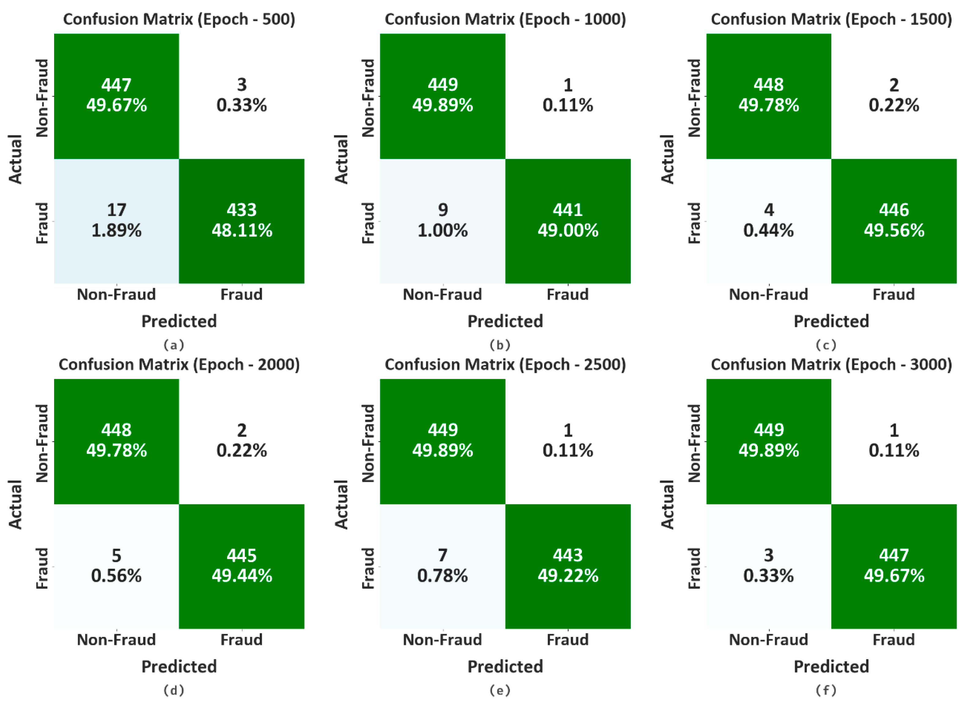
Class	Accuracy	Precision	Sensitivity	Specificity	MCC
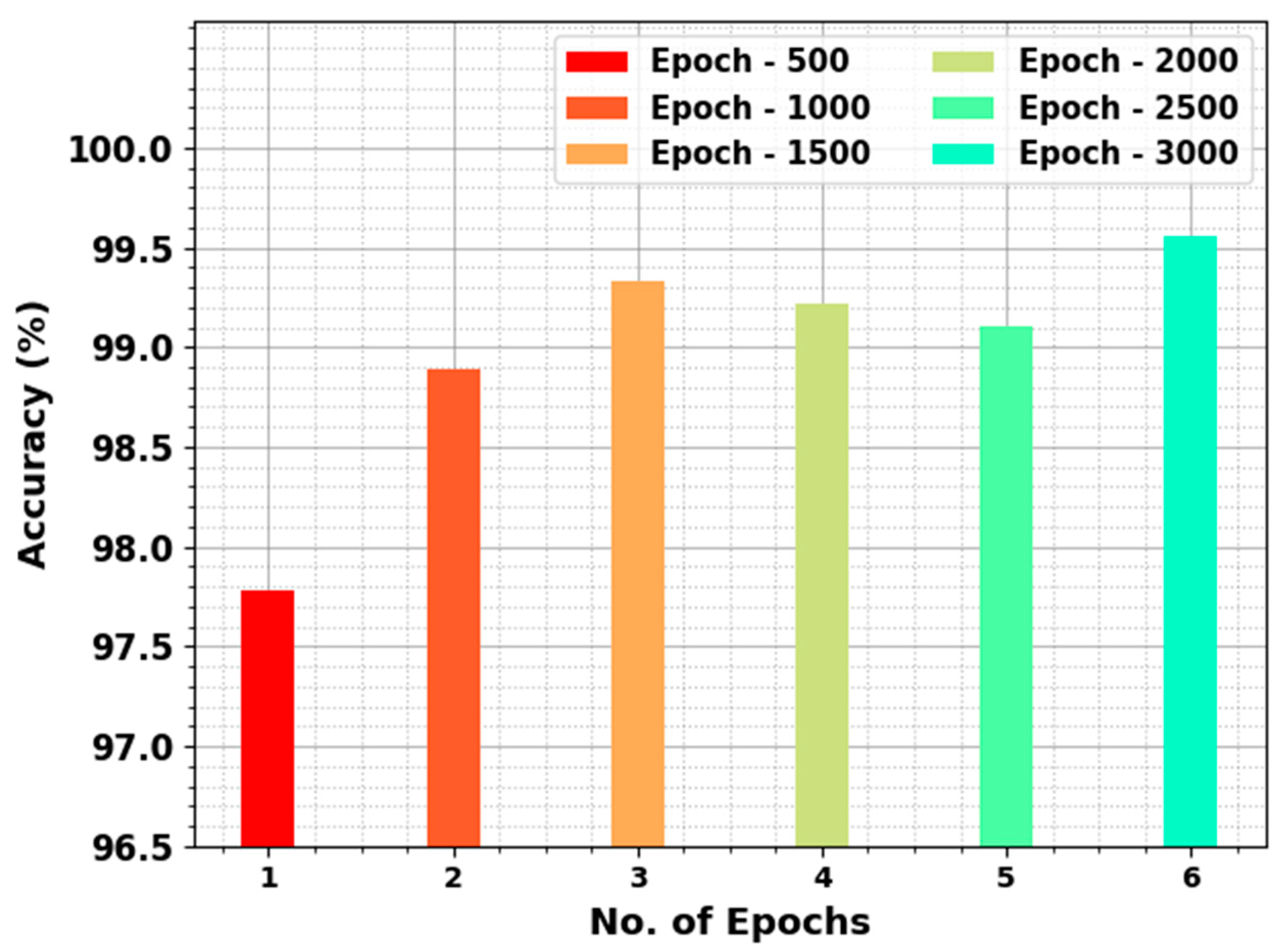
Epoch—500
Non-Fraud	99.33	96.34	99.33	96.22	95.60
Fraud	96.22	99.31	96.22	99.33	95.60
Average	97.78	97.82	97.78	97.78	95.60
Epoch—1000
Non-Fraud	99.78	98.03	99.78	98.00	97.79
Fraud	98.00	99.77	98.00	99.78	97.79
Average	98.89	98.90	98.89	98.89	97.79
Epoch—1500
Non-Fraud	99.56	99.12	99.56	99.11	98.67
Fraud	99.11	99.55	99.11	99.56	98.67
Average	99.33	99.33	99.33	99.33	98.67
Epoch—2000
Non-Fraud	99.56	98.90	99.56	98.89	98.45
Fraud	98.89	99.55	98.89	99.56	98.45
Average	99.22	99.22	99.22	99.22	98.45
Epoch—2500
Non-Fraud	99.78	98.46	99.78	98.44	98.23
Fraud	98.44	99.77	98.44	99.78	98.23
Average	99.11	99.12	99.11	99.11	98.23
Epoch—3000
Non-Fraud	99.78	99.34	99.78	99.33	99.11
Fraud	99.33	99.78	99.33	99.78	99.11
Average	99.56	99.56	99.56	99.56	99.11

and Figure 4 report the overall detection performance of the CCFDC-GRFOEL method under a varying number of epochs. The results demonstrate the effective performance of the proposed CCFDC-GRFOEL method on all the epochs. For example, with 500 epochs, the CCFDC-GRFOEL technique attained an average $acc{u}_y$ of 97.78%, a $pre{c}_n$ of 97.82%, a $sen{s}_y$ of 97.78%, a $spe{c}_y$ of 97.78%, and an MCC of 95.60%. In parallel, with 1,500 epochs, the CCFDC-GRFOEL method reached an average $acc{u}_y$ of 99.33%, a $pre{c}_n$ of 99.33%, a $sen{s}_y$ of 99.33%, a $spe{c}_y$ of 99.33%, and an MCC of 98.67%. At the same time, with 3,000 epochs, the CCFDC-GRFOEL algorithm accomplished an average $acc{u}_y$ of 99.56%, a $pre{c}_n$ of 99.56%, a $sen{s}_y$ of 99.56%, a $spe{c}_y$ of 99.56%, and an MCC of 99.11%.

Figure 5 shows the performance of the CCFDC-GRFOEL approach in both training and validation processes on the test dataset. The figure highlights that the CCFDC-GRFOEL method obtained the maximum outcome values over epochs. Furthermore, the maximum validation outcomes over training accuracy demonstrate that the CCFDC-GRFOEL approach efficiently learnt from the test dataset.

The loss analysis results of the CCFDC-GRFOEL method during training and validation phases upon the test dataset are shown in Figure 6. The outcome illustrates that the CCFDC-GRFOEL approach obtained closer training and validation loss values.

A detailed PR analysis was conducted for the CCFDC-GRFOEL technique using the test dataset, and the results are shown in Figure 7. The experimental outcomes illustrate that the CCFDC-GRFOEL model produced the maximum PR values. In addition to this, the CCFDC-GRFOEL approach obtained the maximum PR values on all the classes.

In Figure 8, the ROC analysis curve obtained via the CCFDC-GRFOEL technique on the test dataset is shown. The figure suggests that the CCFDC-GRFOEL model produced better ROC values. In addition to this, the CCFDC-GRFOEL approach attained the maximum ROC values for all the classes.

The experimental results indicate that the existing techniques such as DSGBT, DTGBT, DTDS, RFGBT, MLP, DT, and the DTNB models obtained the least $acc{u}_y$ values, such as 98.25%, 98.99%, 98.90%, 98.93%, 98.03%, 99.91%, and 98.30%. Simultaneously, the OCSODL-CCFD method accomplished a closer performance with an $acc{u}_y$ of 99.23%. However, the CCFDC-GRFOEL method achieved the maximum $acc{u}_y$ of 99.56%. These outcomes confirm the promising outcomes of the CCFDC-GRFOEL technique over other classifier algorithms.

5. Conclusions

In the current study, a new CCFDC-GRFOEL method has been developed for both the recognition and classification of credit card fraud. The presented CCFDC-GRFOEL technique follows a three-stage process encompassing Z-score normalization, GRFO-based feature subset selection, an ensemble-learning classifier, and POA-based parameter tuning. In order to improve the classification results, the CCFDC-GRFOEL applies the GRFO-FSS approach, which selects a set of features. The ensemble-learning process, comprising ELM, AE, and BiLSTM models, is applied for the detection of fraudulent transactions. Finally, the POA is utilized as a parameter optimizer for all three classifiers. The CCFDC-GRFOEL technique was experimentally validated using a credit card transaction dataset, sourced from the Kaggle repository. The simulation results established the outstanding performance of the proposed technique, while the outcomes from the comprehensive comparison analysis validated the superiority of the CCFDC-GRFOEL technique over other existing approaches. In the future, the Reinforcement Learning (RL) techniques can be applied to design adaptive fraud detection systems that learn from feedback and take suitable actions to prevent the fraud in real-time. By framing the fraud detection problem as a sequential decision-making process, the RL models can optimize the strategies to handle the transactions based on their risk scores.

References

- Strelcenia, E.; Prakoonwit, S. Improving Classification Performance in Credit Card Fraud Detection by Using New Data Augmentation. AI 2023, 4, 172–198. [Google Scholar] [CrossRef]
- Han, S.; Zhu, K.; Zhou, M.; Cai, X. Competition-driven multimodal multiobjective optimization and its application to feature selection for credit card fraud detection. IEEE Trans. Syst. Man Cybern. Syst. 2022, 52, 7845–7857. [Google Scholar] [CrossRef]
- Zhang, X.; Han, Y.; Xu, W.; Wang, Q. HOBA: A novel feature engineering methodology for credit card fraud detection with a deep learning architecture. Inf. Sci. 2021, 557, 302–316. [Google Scholar] [CrossRef]
- Fanai, H.; Abbasimehr, H. A novel combined approach based on deep Autoencoder and deep classifiers for credit card fraud detection. Expert Syst. Appl. 2023, 217, 119562. [Google Scholar] [CrossRef]
- Alam, M.N.; Podder, P.; Bharati, S.; Mondal, M.R.H. Effective machine learning approaches for credit card fraud detection. In Innovations in Bio-Inspired Computing and Applications: Proceedings of the 11th International Conference on Innovations in Bio-Inspired Computing and Applications (IBICA 2020) Held during December 16–18, 2020; Springer International Publishing: Berlin/Heidelberg, Germany, 2021; Volume 11, pp. 154–163. [Google Scholar]
- Chang, V.; Di Stefano, A.; Sun, Z.; Fortino, G. Digital payment fraud detection methods in digital ages and Industry 4.0. Comput. Electr. Eng. 2022, 100, 107734. [Google Scholar] [CrossRef]
- Mustaqim, A.Z.; Adi, S.; Pristyanto, Y.; Astuti, Y. The effect of recursive feature elimination with cross-validation (RFECV) feature selection algorithm toward classifier performance on credit card fraud detection. In Proceedings of the 2021 International Conference on Artificial Intelligence and Computer Science Technology (ICAICST), Yogyakarta, Indonesia, 29–30 June 2021; pp. 270–275. [Google Scholar]
- Malik, E.F.; Khaw, K.W.; Belaton, B.; Wong, W.P.; Chew, X. Credit card fraud detection using a new hybrid machine learning architecture. Mathematics 2022, 10, 1480. [Google Scholar] [CrossRef]
- Fragkos, G.; Minwalla, C.; Plusquellic, J.; Tsiropoulou, E.E. Age Appropriate Digital Services for Young People: Major Reforms. IEEE Consum. Electron. Mag. 2021, 10, 81–89. [Google Scholar] [CrossRef]
- Sharma, P.; Banerjee, S.; Tiwari, D.; Patni, J.C. Machine learning model for credit card fraud detection-a comparative analysis. Int. Arab J. Inf. Technol. 2021, 18, 789–796. [Google Scholar] [CrossRef]
- Prabhakaran, N.; Nedunchelian, R. Oppositional Cat Swarm Optimization-Based Feature Selection Approach for Credit Card Fraud Detection. Comput. Intell. Neurosci. 2023, 2023, 2693022. [Google Scholar] [CrossRef] [PubMed]
- Ahmad, H.; Kasasbeh, B.; Aldabaybah, B.; Rawashdeh, E. Class balancing framework for credit card fraud detection based on clustering and similarity-based selection (SBS). Int. J. Inf. Technol. 2023, 15, 325–333. [Google Scholar] [CrossRef]
- Gradxs, G.P.B.; Rao, N. Behaviour Based Credit Card Fraud Detection Design And Analysis By Using Deep Stacked Autoencoder Based Harris Grey Wolf (Hgw) Method. Scand. J. Inf. Syst. 2023, 35, 1–8. [Google Scholar]
- Ileberi, E.; Sun, Y.; Wang, Z. A machine learning based credit card fraud detection using the GA algorithm for feature selection. J. Big Data 2022, 9, 1–17. [Google Scholar] [CrossRef]
- Kajal, D.; Kaur, K. Credit card fraud detection using imbalance resampling method with feature selection. Int. J. 2021, 10, 2061–2071. [Google Scholar]
- Poongodi, K.; Kumar, D. Support vector machine with information gain based classification for credit card fraud detection system. Int. Arab J. Inf. Technol. 2021, 18, 199–207. [Google Scholar]
- Benchaji, I.; Douzi, S.; El Ouahidi, B.; Jaafari, J. Enhanced credit card fraud detection based on attention mechanism and LSTM deep model. J. Big Data 2021, 8, 1–21. [Google Scholar] [CrossRef]
- Velicheti, S.S.; Pavan, A.S.H.; Reddy, B.T.; Srikala, N.V.; Pranay, R.; Kannaiah, S.K. The Hustlee Credit Card Fraud Detection using Machine Learning. In Proceedings of the 2023 7th International Conference on Computing Methodologies and Communication (ICCMC), Erode, India, 21–23 February 2023; pp. 139–144. [Google Scholar]
- Shyamala Devi, M.; Arun Pandian, J.; Ramesh, P.S.; Prem Chand, A.; Raj, A.; Raj, A.; Thakur, R.K. Oversampled Deep Fully Connected Neural Network Towards Improving Classifier Performance for Fraud Detection. In Advances in Data and Information Sciences: Proceedings of ICDIS 2022; Springer Nature: Singapore, 2022; pp. 363–371. [Google Scholar]
- Jiang, S.; Dong, R.; Wang, J.; Xia, M. Credit Card Fraud Detection Based on Unsupervised Attentional Anomaly Detection Network. Systems 2023, 11, 305. [Google Scholar] [CrossRef]
- Makkineni, N.; Ciripuram, A.; Subhani, S.; Kakulapati, V. Fraud Detection of AD Clicks Using Machine Learning Techniques. J. Sci. Res. Rep. 2023, 29, 84–89. [Google Scholar] [CrossRef]
- Nalluri, V.; Chang, J.R.; Chen, L.S.; Chen, J.C. Building prediction models and discovering important factors of health insurance fraud using machine learning methods. J. Ambient. Intell. Humaniz. Comput. 2023, 14, 9607–9619. [Google Scholar] [CrossRef]
- Reddy, C.S.R.; Prasanth, B.V.; Chandra, B.M. Active power management of grid-connected PV-PEV using a Hybrid GRFO-ITSA technique. Sci. Technol. Energy Transit. 2023, 78, 7. [Google Scholar] [CrossRef]
- Zhu, H.; Li, D.; Yang, M.; Ye, D. Prediction of Microstructure and Mechanical Properties of Atmospheric Plasma-Sprayed 8YSZ Thermal Barrier Coatings Using Hybrid Machine Learning Approaches. Coatings 2023, 13, 602. [Google Scholar] [CrossRef]
- Zhu, H.; Shang, Y.; Wan, Q.; Cheng, F.; Hu, H.; Wu, T. A Model Transfer Method among Spectrometers Based on Improved Deep Autoencoder for Concentration Determination of Heavy Metal Ions by UV-Vis Spectra. Sensors 2023, 23, 3076. [Google Scholar] [CrossRef] [PubMed]
- Du, S.; Li, T.; Yang, Y.; Horng, S.J. Deep air quality forecasting using hybrid deep learning framework. IEEE Trans. Knowl. Data Eng. 2019, 33, 2412–2424. [Google Scholar] [CrossRef]
- Rezk, H.; Olabi, A.G.; Abdelkareem, M.A.; Alahmer, A.; Sayed, E.T. Maximizing Green Hydrogen Production from Water Electrocatalysis: Modeling and Optimization. J. Mar. Sci. Eng. 2023, 11, 617. [Google Scholar] [CrossRef]
- Available online: https://www.kaggle.com/datasets/mlg-ulb/creditcardfraud (accessed on 21 February 2023).