Article

Supply and Demand Patterns Investigations of Water Supply Services Based on Ecosystem Service Flows in a Mountainous Area: Taihang Mountains Case Study

1
Key Laboratory of Agricultural Water Resources, Center for Agricultural Resources Research, Institute of Genetic and Developmental Biology, Chinese Academy of Sciences, Shijiazhuang 050021, China
2
College of Horticulture Science and Technology, Hebei Normal University of Science & Technology, Qinhuangdao 066004, China
3
College of Advanced Agricultural Sciences, University of Chinese Academy of Sciences, Beijing 100049, China
*
Author to whom correspondence should be addressed.
These authors contributed equally to this work.
Sustainability 2023, 15(17), 13248; https://doi.org/10.3390/su151713248
Submission received: 13 July 2023 / Revised: 27 August 2023 / Accepted: 31 August 2023 / Published: 4 September 2023

Abstract

:
The study of water service supply, demand, and flow in the Taihang Mountains in China can elucidate its supply and demand patterns, which are important for the sustainable utilization of water resources. We chose Gangnan Reservoir Basin in the Taihang Mountains as the research area. First, we evaluated the supply and demand of water supply services using the InVEST model and statistical methods. Then, ecosystem service flows were calculated based on river networks and altitude. Finally, the supply and demand pattern of water supply services based on ecosystem service flows was analyzed. The results showed the following. (1) The total supply and demand of water supply services in Gangnan Reservoir Basin were 8.18 × 10⁸ m3 and 3.52 × 10⁸ m3, respectively. (2) At the sub-basin scale, the minimum flow of both static and dynamic water supply services was the same, and the mean was significantly different. The maximum flow was also significantly different. Static water supply service flows were not significantly correlated with altitude, whereas dynamic water supply service flows were significantly correlated with altitude. (3) The demand area in the supply and demand pattern of water supply services based on dynamic ecosystem service flows was notably less than that based on static ecosystem service flows. The supply and demand patterns of water supply services defined the actual water shortage area, the area that pays for ecosystem services, and the areas of ecosystem service ecological compensation, providing a scientific basis for the safe and rational utilization of water resources in mountainous areas.

1. Introduction

The Taihang Mountains are the source, or upstream area, of many rivers, and are part of the Yellow River Basin and Haihe River Basin in China. They are an important water supply area for the North China Plain [1,2]. Socioeconomic development and climate change have a large impact on water supply services [3]. The Taihang Mountains are an important ecological barrier area of the Beijing, Tianjin, Hebei, and Henan provinces in China. Water shortages have been a key factor restricting vegetation restoration and reconstruction in the Taihang Mountains [4,5]. Zhu et al. [6] analyzed the vertical gradient characteristics of the supply and demand for water supply services in the Taihang Mountains, but the supply and demand patterns of water supply services based on ecosystem service flows remain unclear.
Mountainous areas are known as “water towers”. Water supply services are one of the important ecosystem services provided by mountainous regions, on which a large proportion of the world’s population depends for their water [7,8,9]. China is a mountainous country, with mountainous areas accounting for 65% of its total land area [10]. Mountain areas in China are irreplaceable in terms of water supply services and play a vital role in freshwater supply for themselves and the surrounding lowlands. Water supply services of mountain areas around the world face multiple challenges due to environmental and socio-economic changes. In terms of water supply, mountain ecosystems are vulnerable to rising temperatures due to the amplification of global warming at high altitudes, resulting in melting glaciers and changes in runoff [11]. In terms of water demand, urbanization intensifies the demand for freshwater resources [12]. The changes in water resource supply and demand affect the supply and demand patterns of water supply services [13]. In addition, the vulnerability, diversity, and unique vertical gradient patterns of mountain areas can make defining the supply and demand patterns of water supply services difficult [14,15].
Water supply service research initially focused on water supply evaluation [16,17]. The integrated valuation of ecosystem services and tradeoffs (InVEST) model has been widely applied in water supply service evaluation [18,19,20]. The soil and water assessment tool (SWAT) model is also used in water supply service assessments, and its assessment process has a major focus on hydrological processes [21,22]. The SWAT model requires more complex data than the InVEST model [23,24]. As the relationship between ecosystem services and human welfare becomes increasingly close, the demand for water supply services has become another focus of the field of ecosystem services [25,26,27]. At present, expert knowledge scoring, questionnaire surveying, and statistical analysis based on land use and statistical data have mainly been used to estimate and analyze the temporal and spatial characteristics of water supply service demand [28,29,30,31]. There is a lack of studies on the supply and demand pattern of water supply services in the context of water supply service flows [32,33].
There is no clear definition of water supply service flow, and research has focused on the spatial flow of water supply services. Zhu et al. [19] defined the water security index (WSI) as the ratio of freshwater service provision and consumption, which serves as the metric linking ecosystem services and human demand. To compare the conventional static and dynamic water flow models, they calculated the WSI both with and without considering the amount of upstream freshwater services. The results showed that there was no significant difference between dynamic and static WSI in the forest belt, whereas there was a significant difference outside the forest belt. Sun et al. [24] studied the supply and demand patterns of water supply services considering the spatial flow of water supply services and defined the freshwater supply area, the freshwater benefit area, and neither supply nor benefit area of the Yellow River Basin. In addition to supply and demand, the analysis of water supply service flows in the above studies also includes the inflow of upstream water supply services. It is not clear how the inflow of upstream water supply services will affect the supply and demand patterns of water supply services [24,34].
This study chose Gangnan Reservoir Basin in the Taihang Mountains as a case study. We attempted to define the concept of water supply service flows and quantitatively evaluate the characteristics of static and dynamic water supply service flows, then analyze the supply and demand patterns of water supply services based on ecosystem service flows. First, the supply of water supply services was modeled using InVEST and water consumption services were calculated using available statistical data. Second, the spatial flow of the water ecosystem service was quantified using a simplified water flow model. Finally, we defined the supply and demand patterns of water supply services based on ecosystem service flows. The main objectives of this paper are (1) to evaluate the spatial distribution characteristics of water supply services’ supply and demand; (2) to quantify the spatial flow of water resources in different sub-basins; and (3) to identify which areas are supply areas and which are demand areas.

2. Materials and Methods
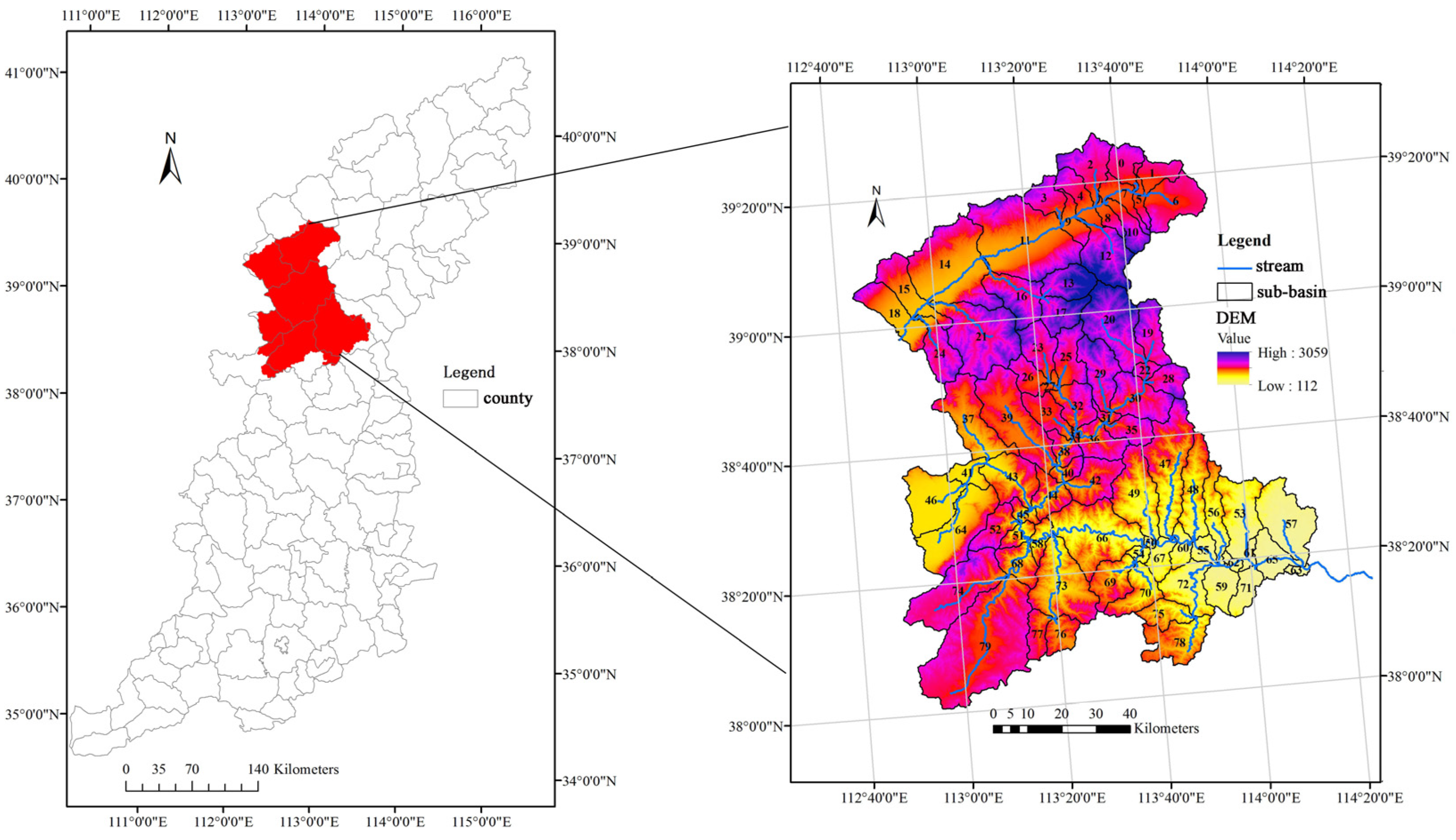
2.1. Study Area

The Taihang Mountains, a natural barrier and important water source of the North China Plain, are located in the central and eastern part of China. It extends across 101 counties in four provinces (Beijing, Hebei, Shanxi, and Henan) (Figure 1), covering an area of about 14,000 km2. They are steep in the east and gentle in the west, high in the north and low in the south. The highest elevation is about 3000 m, the lowest elevation is about 10 m, and the average elevation is 860 m. The Taihang Mountains are influenced by the East Asian Monsoon climate. The summer is warm and rainy, and the winter is cold and dry. The average annual rainfall is 570 mm, and the average annual temperature is 10 °C. The main land use types are cultivated land, forest land, grassland, and buildings, accounting for more than 90% of the total area [35].
The Gangnan Reservoir Basin is located in the central and western part of the Taihang Mountains, with an elevation span of 112–3059 m. The main land use type is similar to that of the Taihang Mountains [36], and it is a typical representative basin of the Taihang Mountains. The basin is located at 38°00′–39°30′ E and 112°40′–114°20′ N, encompassing seven counties in Shanxi and Hebei and covering an area of about 11,864 km2. The elevation is higher in the middle and lower in the north and south, with the highest elevation being 3059 m and the lowest being about 112 m. It is divided into 80 sub-basins, and the water resources of the sub-basins flow through the river network (Figure 1).

2.2. Data Sources

The land use data of Gangnan Reservoir Basin in 2015 were interpreted using a 30 m resolution Landsat TM (Table 1) satellite image, which was provided by the National Basic Research Program (973 Program) of China. The DEM data were downloaded from the Resources and Environment Science Data Center of the Chinese Academy of Sciences (http://www.resdc.cn) (accessed on 6 May 2022) and were used for topographic analysis and watershed division. Precipitation data for 2013–2017 were obtained from provincial weather bureaus. The global MODIS land evapotranspiration product data (MOD16) released by the NASA Earth Observation System were used for potential evapotranspiration data from 2013 to 2017. Soil attribute data were derived from the National Earth System Science Data Sharing Service Platform (http://www.geodata.cn) (accessed on 6 July 2020) and were used to calculate the water available to plants. The runoff data of the basin from 2013 to 2017 were derived from the Annual Report of Hebei Soil and Water Conservation Bulletin, which was used to verify the water yield results. Data on water demand per person per year came from the water resources communique of Shanxi and Hebei provinces from 2013 to 2017. The grid data of the population in 2015 were derived from the National Earth System Science Data Sharing Service Platform (http://www.geodata.cn) (accessed on 6 June 2018).

2.3. Research Methodology

To reveal the supply and demand patterns of water supply services in Gangnan Reservoir Basin, we performed the following data analyses. The databases, computational tools, methods, main research content, and overall framework are shown in Figure 2.

2.3.1. Assessment of Water Supply Service Supply

We employed the water yield module in InVEST to calculate the water supply services based on the following Equations (1)–(3) [31,37]. The InVEST model was developed by Stanford University. The water yield module uses a basic hydrological model that subtracts evapotranspiration from combined infiltration and runoff without differentiating between surface, subsurface, and base flow.
W Y x = 1 A E T x P x × P x  
A E T x P x = 1 + P E T x P x 1 + P E T x P x w 1 w
w = Z × A W C x P x + 1.25  
In the equation, W Y x   is the average annual water supply on grid x; P x   is the average annual precipitation on grid x; A E T x   is the average annual actual evapotranspiration on grid x; w is a dimensionless non-physical parameter that characterizes the natural climatic soil properties; Z is the Zhang coefficient (seasonality factor), which captures the local precipitation patterns and additional hydrogeological characteristics, which should be adjusted based on the simulation results of water yield and the annual runoff observations in the model validation; and A W C x is the soil effective water content (mm) and is determined based on the plant available water content, as well as the maximum root depth of the soil and the minimum root depth of the plant.
Based on an assessment of supply of water supply services at the grid scale, ArcGIS 10.2 software was used to statistically analyze the supply of water supply services at the sub-basin scale.

2.3.2. Model Verification

Water services supply ( W Y x   ) is the sum of inflow and water supply service demand ( W D x ). The average annual inflow and water demand of Gangnan Reservoir Basin from 2013 to 2017 were used to verify the simulation results. The seasonality constant (Z) was calibrated in order to obtain an optimized output. When the Z of the InVEST model was 5.86, the results of the water yield simulation were the best. The total simulated water yield was 8.18 × 10⁸ m3, and the total observed water yield (4.63 × 10⁸ m3 water inflow and 3.52 × 10⁸ m3 water consumption) was 8.15 × 10⁸ m3, with an error of only 0.03 × 10⁸ m3. The InVEST model has 99.6% accuracy, indicating its good performance.

2.3.3. Assessment of Water Supply Service Demand

The water supply services demand was obtained by multiplying the municipal comprehensive water consumption per person per year by population, and the population raster data of 2015 were used to realize the spatialization of the demand. The calculation Equation (4) is as follows [6]:
W D x = H B a v e r a g e × P O P x  
In the equation, W D x   represents the annual water demand on grid x; H B a v e r a g e represents the annual comprehensive water consumption of each person at the municipal level; and P O P x represents the number of people on grid x.
Based on an assessment of the demand for water supply services at the grid scale, ArcGIS 10.2 software was used to statistically analyze the demand for water supply services at the sub-basin scale.

2.3.4. Quantification of Water Supply Service Flows

The flow pathways and direction were traced via the downhill and downstream runoff according to a digital elevation model and river network data. Matrices were used to simulate flow. The supply matrix was populated with the total amount of water supply service at the sub-basin scale (Figure 3a). The demand matrix showed the spatial distribution of human demand for water, also at the sub-basin scale (Figure 3b). Figure 3c showed a simulation of the flow of water supply services. The static water supply service surplus (SWS) was the residual amount of water supply service after balancing water demand (Figure 3d). The dynamic water supply service surplus (DWS) was the residual amount of water supply service after balancing water demand (WD) and upstream DWS (Figure 3e).
We analyzed the water supply service flow from both static and dynamic perspectives. We assumed that each sub-basin preferentially uses its own water yield (WY) to balance its own demand. Static water supply service flow (SWF) is the static water supply service surplus (SWS). An SWS ≥ 0 of the sub-basin indicates a supply area, and an SWS < 0 of the sub-basin indicates a demand area. Dynamic water supply service flow (DWF) is the dynamic water supply service surplus (DWS). A DWS ≥ 0 of the sub-basin indicates a supply area, and a DWS < 0 of the sub-basin indicates a demand area.

2.3.5. Global Spatial Autocorrelation of Water Supply Service Supply, Demand, and Flow

Global spatial autocorrelation is the analysis and description of the overall spatial features of geographical elements in a research area and can clearly represent the degree of spatial interdependence of geographical variables. A common measure of global spatial autocorrelation is the global Moran’s I index, which lies in the range of [−1, 1]. If its value is positive, it indicates that there is a positive spatial autocorrelation; that is, the research object and the neighboring object have the same change trend. A negative number indicates that there is a negative spatial autocorrelation; that is, the trend of change of the research object and the neighboring object are the opposite. A zero indicates that there is no spatial autocorrelation. The global Moran’s I is calculated as in (5) [38]:
I = N i = 1 N j = 1 N w i j ( x i x ¯ ) ( x j x ¯ ) ( i = 1 N j = 1 N w i j ) i = 1 N ( x i x ¯ ) 2  
where N equals the number of observations; wij is the weight between locations i and j; xi and xj are the values at locations i and j; and x ¯   is the average over all locations of the variable.

3. Results

3.1. Water Supply Service Supply and Demand

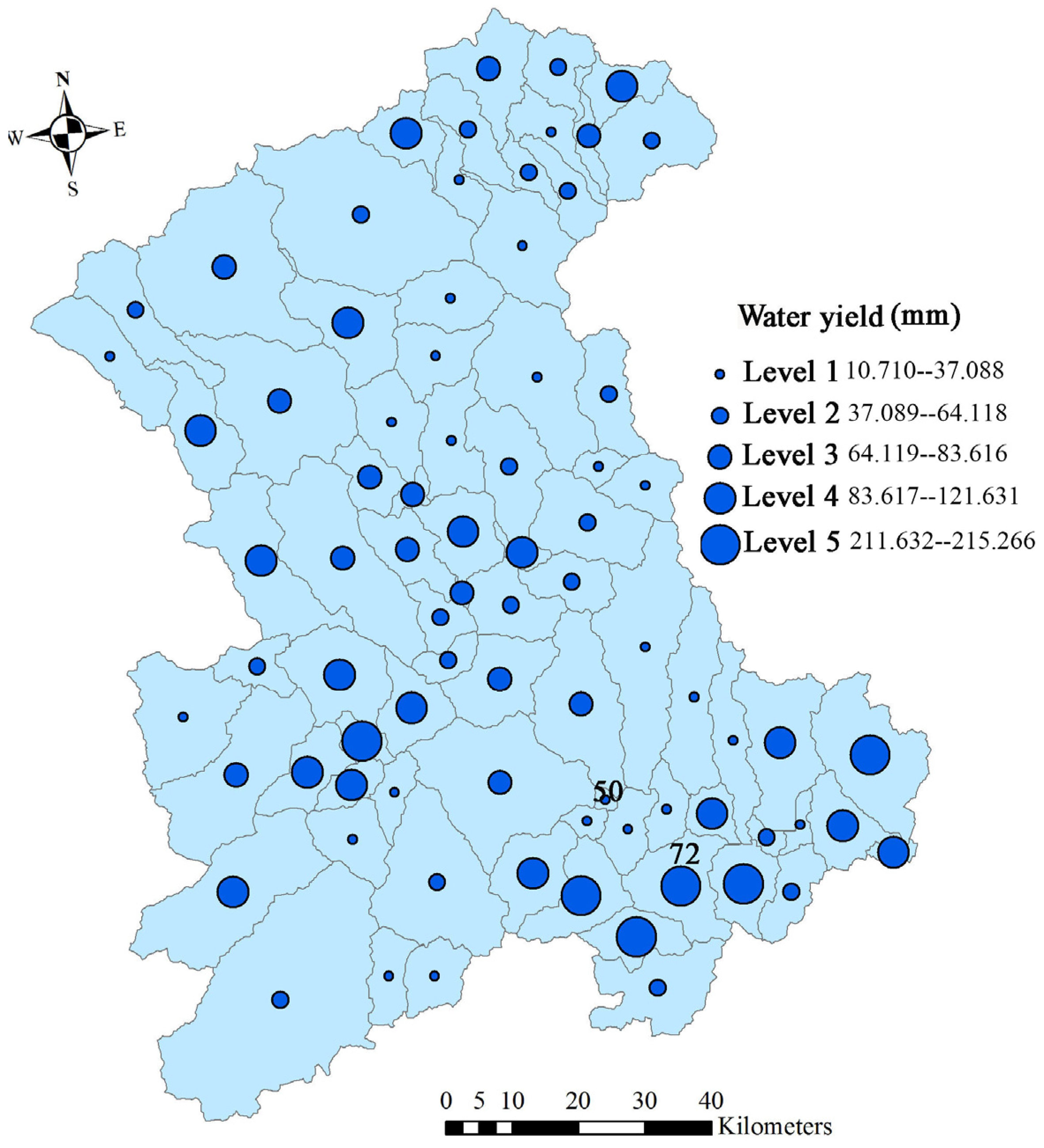
3.1.1. Water Supply Service Supply

The average water yield of Gangnan Reservoir Basin was found to be 69 mm. On the scale of sub-basin, sub-basin 72 had the largest water yield of 215 mm, while sub-basin 50 had the smallest water yield of 11 mm. The number of sub-basins at level 1 of water yield accounted for the largest proportion, with a total of 24 sub-basins, followed by level 2, with a total of 20 sub-basins. The number of sub-basins at level 5, with the maximum water yield, was the smallest, with only six sub-basins. The number of sub-basins at level 3 and level 4 of water yield was 14 and 17 sub-basins, respectively (Figure 4). The global Moran’s I index value of average water yield is 0.16, and the Z test value is 2.65, with p = 0.008 (p < 0.05), indicating that there is a significant positive spatial autocorrelation of average water yield. The total water yield of Gangnan Reservoir Basin was 8.18 × 10⁸ m3. On the scale of sub-basin, sub-basin 57 had the largest total water yield (4.46 × 10⁷ m3), while sub-basin 50 had the smallest total water yield (1.03 × 10⁵ m3). The number of sub-basins at level 5 was the largest, with 12 sub-basins, followed by level 2, with 11 sub-basins (Figure 5). The global Moran’s I index value and Z test value of total water yield were 0.11 and 1.91, with p = 0.57 (p > 0.05), indicating that there was no significant global spatial autocorrelation of water yield.

3.1.2. Water Supply Service Demand

The catchment of Gangnan Reservoir covers four cities, and the annual water consumption per person is shown in Table 2. The annual water consumption per person in Shijiazhuang city was the largest. There are 19 sub-basins in Shijiazhuang city, namely 47, 48, 49, 50, 53, 54, 55, 56, 57, 59, 60, 61, 62, 63, 65, 67, 70, 71, and 72 (Figure 6). The annual water consumption per person of Yangquan city was the smallest, including nine sub-basins, namely 58, 66, 68, 69, 73, 76, 77, 78, and 79. The annual water consumption per person in Taiyuan city was 175 m3, including one sub-basin (74). The annual water consumption per person in Yizhou city was 209 m3, including 51 sub-basins, accounting for 65% of the total sub-basins (Table 2).
The total demand for water supply service in Gangnan Reservoir Basin was 3.52 × 10⁸ m3. On the scale of sub-basin, sub-basin 64 had the largest water demand (1.75 × 10⁷ m3), while sub-basin 34 had the smallest water demand (1.16 × 10⁵ m3). The number of sub-basins at level 6 accounted for the largest proportion, with a total of 12 sub-basins, followed by level 5 with 11 sub-basins (Figure 6). The global Moran’s I index value of water supply services demand is 0.19 and the Z test value is 3.17, with p = 0.001 (p < 0.05), indicating that there is a significant positive spatial autocorrelation of demand for water supply services.

3.2. Water Supply Service Flows

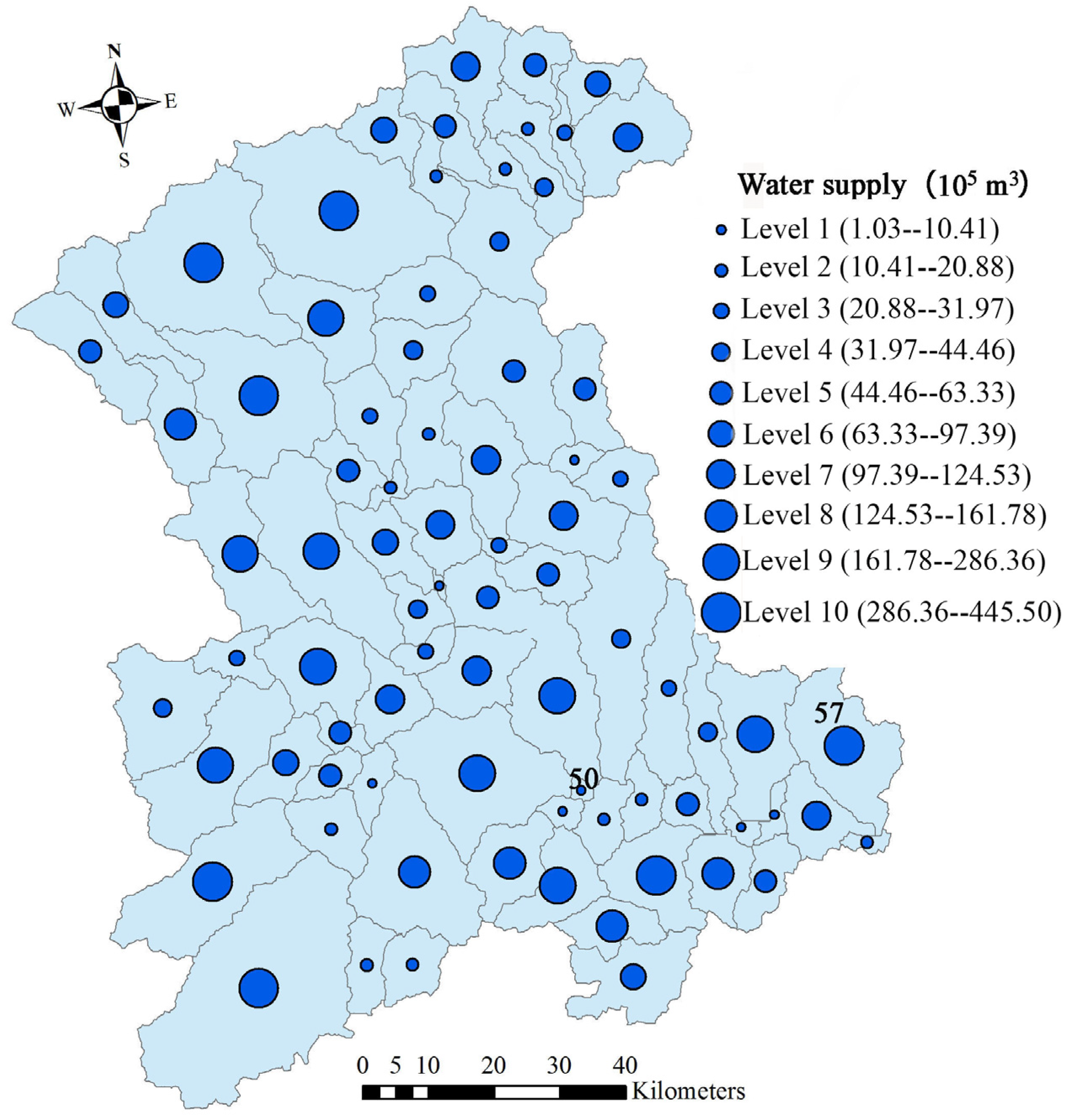
3.2.1. Water Supply Service Flow Characteristics

The minimum static water supply service flow was 2.00 × 10⁵ m3 in sub-basin 23, and the maximum was 3.00 × 10⁷ m3 in sub-basin 79 (Figure 7). The average value of static water supply service flow in all sub-basins was 5.83 × 10⁶ m3. The static water supply service flow of sub-basin 1 was 5.77 × 10⁶ m3, which was closest to the average value. Among the flow levels, level 1 contained the largest number of sub-basins, with 20. This was followed by level 2, with 17, while level 5 had the least, with five.
The dynamic water supply service flow is based on the physical flow process of water, which is characterized by the size and the direction of the flow. The flow direction of water supply service flow was from high altitude to low altitude. Among the flow levels, level 1 contained the largest number of sub-basins, with 29. This was followed by level 2 with 19, and level 5 had the least, with six. The minimum dynamic water supply service flow was 2.00 × 10⁵ m3 in sub-basin 23, and the maximum was 4.61 × 10⁸ m3 in sub-basin 63 (Figure 8). The average value of dynamic water supply service flow in all sub-basins was 7.69 × 10⁷ m3. The dynamic water supply service flow of sub-basin 44 was 8.31 × 10⁷ m3, which was closest to the average value.
In summary, compared with dynamic water supply service flow, static water supply service flow did not exhibit the characteristics of flow direction. For static and dynamic water supply service flows at the sub-basin scale, the minimum flow was not different, whereas the mean and maximum flow differed significantly between static and dynamic water supply service flows. The maximum flow of static water supply service flow was 6.51% of the maximum flow of dynamic water supply service flow. The average flow of static water supply service flow was 7.58% of the average flow of dynamic water supply service flow.

3.2.2. Spatial Distribution Characteristics of Water Supply Service Flows

The global Moran’s I index value and Z test value of static water supply service flow were 0.11 and 1.91, with p = 0.06 (p > 0.05), indicating that there was no significant global spatial autocorrelation. On the vertical gradient, static water supply service flow was negatively correlated with altitude, but not significantly (Figure 9). The average elevations of the sub-basins contained by the water supply service flows at the first, second, third, fourth, and fifth levels were 1204 m, 1170 m, 1206 m, 1139 m, and 930 m, respectively.
The global Moran’s I index value of dynamic water supply service flow was 0.61 and the Z test value was 9.49, with p = 0.000 (p < 0.05), indicating that there was a significant positive spatial autocorrelation. On the vertical gradient, the flow direction of dynamic water supply service flow was from high altitude to low altitude, and there was a significant negative correlation between flow and altitude (Figure 10). The higher the altitude, the smaller the water supply service flow. The average elevation of the sub-basins contained by the water supply service flows at level 1 and level 2 was similar, at 1348 m and 1341 m, respectively. Level 3 had an average elevation of 1181m. Levels 4 and 5 had an average elevation of 1006 m and 452 m, respectively.
In summary, the static and dynamic water supply service flows all have positive spatial autocorrelations. In terms of elevation gradient, both static and dynamic water supply service flows were negatively correlated with altitude. Static water supply service flow demonstrated no significant correlation with altitude, while dynamic water supply service flow had a significant correlation with altitude.

3.3. Characteristics of Supply and Demand Pattern of Water Supply Services Based on Ecosystem Service Flows

In the supply and demand pattern based on static water supply service flow in Gangnan Reservoir Basin, 16 sub-basins were demand areas and the rest were supply areas (Figure 11). A demand area is a sub-basin whose own water yield cannot meet its own demand; that is, SWS < 0. A demand area needs to utilize the water supply services of other sub-basins, which means they need to obtain water supply services. The supply area refers to the water yield of the sub-basin that meets its own demand and has a surplus; that is, SWS ≥ 0, and this area can provide water supply services to other sub-basins. Therefore, the supply area is the potential water supply service supply area, though whether it is the actual supply area depends on the situation.
In the supply and demand pattern based on dynamic water supply service flows in Gangnan Reservoir Basin, six sub-basins were demand areas and the rest were supply areas (Figure 12). The demand area is a sub-basin whose own water yield and upstream inflow of dynamic water supply service surplus cannot meet its own demand; that is, DWS < 0. The demand area constitutes the actual water shortage area. The supply area is a sub-basin whose own water yield and upstream inflow of dynamic water supply service surplus can meet its own demand; that is, DWS ≥ 0. The supply area can provide water supply services. The residual amount of dynamic water supply services in the supply area reflects the potential maximum water supply, which is not the actual water supply due to counting upstream DWS multiple times.
Based on static and dynamic ecosystem service flows, the supply and demand patterns of water supply services exhibited significant differences in Gangnan Reservoir Basin. The number of sub-basins in the supply area and that in the demand area are 64 and 16, respectively, based on static ecosystem service flows. However, the number of sub-basins in the supply area and that in the demand area are 73 and 7, respectively, based on dynamic ecosystem service flows. The demand area in the supply and demand pattern of water supply service based on dynamic ecosystem service flows was evidently less than that based on static ecosystem service flows. Sub-basins 7, 41, 46, 50, 54, 60, 61, 67, and 68 were transformed from demand areas to supply areas. In the supply and demand pattern based on dynamic water supply service flow, only sub-basins 12, 20, 22, 25, 47, 48, and 56 were demand areas, while the other 73 sub-basins were supply areas.

4. Discussion

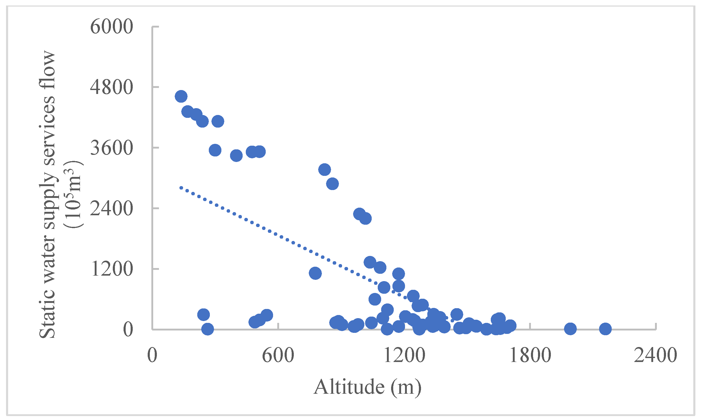
4.1. The Difference between Water Supply Service Flow and Water Physical Flow

Water supply service flow processes can be determined according to physical river flows [19,30]. However, the actual physical flow of water differs from that of the water supply service flow. Ecosystem service flows assumed that after the demand within the region had been met, the remaining ecosystem services would form an ecosystem service flow. Sub-basin 47 of Gangnan Reservoir Basin was determined as the demand area (Figure 9 and Figure 10). There is no dynamic or static water supply and service flow, but there is water physical flow. According to the principle of isotope conservation, the water physical flow characteristics of sub-basin 47 were analyzed using the following Equations (6) and (7) [39]:
f p × δ 18 O p + ( 1 f p ) × δ 18 O h = δ 18 O l
δ 18 O p = i = 1 n w i × δ 18 O p i
In the equation, f p   is the proportion of rainfall in the water volume of low-altitude rivers; 1 f p is the proportion of inflow of high-altitude rivers to the water volume of low-altitude rivers; δ 18 O p is the average oxygen isotope of precipitation;   δ 18 O h is the average oxygen isotope of high-altitude river runoff; δ 18 O l is the mean value of oxygen isotope in low-altitude runoff; w i is the weight of each rainfall; and δ 18 O p i   is the oxygen isotope value of each rainfall. The results showed that 67.48% of the water in the rivers in the mid-mountain zone (600–1400 m) originated from the sub-alpine zone (>1500 m), and the remainder originated from precipitation. We found that 37.66% of the river water in the hilly zone (<500 m) originated from the mid-mountain zone, and the rest originated from precipitation. Therefore, the water supply service flow differed from the water physical flow. The physical flow explains the hydrological process, while the service flow is more focused on value quantification. Future research on water resources should be defined according to the research purpose, namely ecosystem service flow or physical flow.

4.2. Factors Influencing the Supply and Demand Patterns of Water Supply Services

Factors influencing ecosystem service supply and demand include socio-economic factors, such as population density, gross domestic product (GDP), and urban expansion, as well as ecological environmental factors, such as elevation, slope, rainfall, temperature, normalized difference vegetation index (NDVI), and land use [40]. As an ecological environmental factor, land use change is the most important factor affecting the supply and demand of ecosystem services [41]. Socio-economic factors include GDP, resident population, energy consumption, etc. [42]. Delphin et al. [43] found that climate change had a more significant impact on water supply and service supply than other driving factors in two watersheds in Florida, USA. Zhao et al. [44] noted that population had the greatest impact on water supply service demand in Gansu province of China. We selected factors such as elevation, slope, soil layer thickness, rainfall, temperature, NDVI, land use type, population density, and GDP to evaluate the impact of these factors on the ratio of water supply and service demand. The ratio of supply and demand for water supply service is calculated as in (8) [9]:
W r a t i o = W Y i W D i
In the equation, W r a t i o is the ratio of supply and demand; W Y i is the water supply service supply of the sub-basin; and W D i is the water supply service demand of the sub-basin. The results showed that soil depth, GDP, and population density were significantly negatively correlated with the supply and demand ratio, while slope and forest area ratio were significantly positively correlated with the supply and demand ratio. Therefore, the factors affecting the supply and demand for water supply services were mainly soil depth, GDP, population density, slope, and forest area in Gangnan Reservoir Basin. There are some similarities and differences with previous studies. In summary, the main influencing factors of water supply and demand patterns differed in different regions and thus need to be analyzed according to the actual situation.

4.3. Suggestions for the Rational Utilization of Water Resources Based on the Supply and Demand Patterns of Water Supply Services

Water supply services are closely related to the demand for water and electricity and the irrigation of farmlands. Water supply services have become an important ecosystem service. The supply and demand patterns based on static water supply service flows provide a scientific basis for the policy formulation of water supply service use payment and ecological compensation. The demand area in supply and demand patterns based on static water supply service flows can be defined as the water supply service use area. The supply area can be determined as the potential water supply service ecological compensation area. The quantification of service payment and compensation can be determined according to the size of the static water supply service flow [45]. The supply and demand patterns based on dynamic water supply service flows can be used to identify water supply service shortage areas, namely the demand area. In order to support people’s livelihoods, these areas can be identified as priority water resource management areas [18]. Mountainous areas can reduce the restoration activities of artificial forest land in the upper reaches, thus reducing the evapotranspiration of forest land and increasing the runoff, ultimately increasing the supply of water supply and services [46,47]. Huang et al. [46] found that the average runoff from cultivated fallow land was very high, reaching 10.3% of the seasonal rainfall, and the evapotranspiration of two kinds of forest and one kind of shrub was 5.2%, 6.6%, and 8.4% higher than that of natural grassland. Water-wise agricultural irrigation and irrigation water efficiency should be encouraged to reduce the demand for water supply services [48,49]. Gao et al. [48] found that the practice of 20% deficit irrigation, furrow irrigation, and mulching results in no reduction yield and a relatively low water footprint, which can save up to 20% of irrigation water and 8–12% of effective precipitation in an irrigation district, which is the optimal balance point between the yield and water consumption of the two crops. We should also focus on water recycling, such as rainwater collection and the recycling of reclaimed water, which would ultimately reduce the demand for water supply and services. Yao et al. [50] found that the high level of actual available rainwater has been expanding to the western region with dense grassland coverage in the Yellow River Basin in China.

5. Conclusions

In this study, we analyzed the supply, demand, and flow of water supply services in Gangnan Reservoir Basin using the InVEST model and statistical data via the GIS platform to determine the pattern of the supply and demand of water supply services in the basin. This study showed that the total water yield and water demand of the basin were 8.18 × 10⁸ m3 and 3.52 × 10⁸ m3. The total water yield and water demand have positive spatial autocorrelation at the sub-basin scale. At the sub-basin scale, the minimum flow of static and dynamic water supply services was the same, whereas the maximum and the mean flow were significantly different. The static and dynamic water supply service flows both have positive spatial autocorrelations. They were negatively correlated with altitude. Based on static and dynamic ecosystem service flows, the supply and demand patterns of water supply services exhibited significant difference in the basin. The demand area in the supply and demand pattern of water supply service based on dynamic ecosystem service flows was obviously less than that based on static ecosystem service flows. In the supply and demand pattern of water supply services based on dynamic ecosystem service flows, demand areas represent the actual water shortage area. In the supply and demand patterns of water supply services based on static ecosystem service flows, demand areas represent the area that pays for ecosystem services and supply areas represent potential areas of ecosystem service ecological compensation. The government can provide the appropriate amount of ecological compensation based on the flow of water supply services and the determined ecosystem service compensation area. Our study provides a scientific basis for the safe and rational utilization and distribution of water resources in mountainous areas.

Author Contributions

Conceptualization, H.G. and T.F.; methodology, H.G.; software, J.Z.; validation, T.F. and J.L.; formal analysis, H.G.; investigation, F.Q.; resources, T.F.; data curation, M.Z.; writing—original draft preparation, H.G.; writing—review and editing, T.F.; visualization, F.W.; supervision, J.L.; project administration, J.L.; funding acquisition, J.L. All authors have read and agreed to the published version of the manuscript.

Funding

This research was funded by the Science & Technology Fundamental Resources Investigation Program (No. 2022FY100104) and the Natural Science Foundation of Hebei Province (No. D2020407002).

Institutional Review Board Statement

Not applicable.

Informed Consent Statement

Not applicable.

Data Availability Statement

The data presented in this study are available on request from the corresponding author.

Conflicts of Interest

The authors declare no conflict of interest.

References

  1. Song, X.F.; Li, F.D.; Liu, C.M.; Tang, C.Y.; Zhang, Q.Y.; Zhang, W.J. Water cycle in Taihang Mountain and its recharge to groundwater in North China Plain. J. Nat. Resour. 2007, 22, 398–408. (In Chinese) [Google Scholar]
  2. Hu, Y.S.; Zhai, H.B.; Tian, Y. Analysis on sustainability of Taihang Mountain greening construction. For. Econ. 2017, 39, 48–52. (In Chinese) [Google Scholar]
  3. Huang, M.D.; Xiao, Y.; Xu, J.; Liu, J.Y.; Wang, Y.Y.; Gan, S.; Lv, S.X.; Xie, G.D. A review on the supply-demand relationship and spatial flows of ecosystem services. J. Resour. Ecol. 2022, 13, 925–935. [Google Scholar]
  4. Yang, Y.H.; Wang, Z.P.; Sakura, Y.S.; Tang, C.Y.; Shindo, S.Z. Effects of global warming on productivity and soil moisture in Taihang Mountain. Chin. J. Appl. Ecol. 2002, 13, 667–671. (In Chinese) [Google Scholar]
  5. Song, X.F.; Wang, P.; Yu, J.J.; Liu, X.; Liu, J.R.; Yuan, R.Q. Relationships between precipitation, soil water and groundwater at Chongling catchment with the typical vegetation cover in the Taihang mountainous region, China. Environ. Earth Sci. 2011, 62, 787–796. [Google Scholar] [CrossRef]
  6. Zhu, J.J.; Liu, J.T.; Liang, H.Z.; Gao, H.; Liu, P. Vertical gradients of water supply and demand in Taihang Mountains, China. Chin. J. Appl. Ecol. 2019, 30, 472–480. (In Chinese) [Google Scholar]
  7. Meisch, C.; Schirpke, U.; Huber, L.; Rüdisser, J.; Tappeiner, U. Assessing freshwater provision and consumption in the alpine space applying the ecosystem service concept. Sustainability 2019, 11, 1131. [Google Scholar] [CrossRef]
  8. Grêt-Regamey, A.; Weibel, B. Global assessment of mountain ecosystem services using earth observation data. Ecosyst. Serv. 2020, 46, 101213. [Google Scholar] [CrossRef]
  9. Immerzeel, W.W.; Lutz, A.F.; Andrade, M.; Bahl, A.; Biemans, H.; Bolch, T.; Hyde, S.; Brumby, S.; Davies, B.J.; Elmore, A.C.; et al. Importance and vulnerability of the world’s water towers. Nature 2020, 577, 364–384. [Google Scholar] [CrossRef]
  10. Deng, W.; Dai, E.F.; Jia, Y.W.; Chen, H.S.; Xiong, D.H.; Shi, P.L. Spatiotemporal coupling characteristics, effects and their regulation of water and soil elements in mountainous area. Mt. Res. 2015, 33, 513–520. (In Chinese) [Google Scholar]
  11. Rogora, M.; Frate, L.; Carranza, M.L.; Freppaz, M.; Stanisci, A.; Bertani, I.; Bottarin, R.; Brambilla, A.; Canullo, R.; Carbognani, M.; et al. Assessment of climate change effects on mountain ecosystems through a cross-site analysis in the Alps and Apennines. Sci. Total Environ. 2018, 624, 1429–1442. [Google Scholar] [CrossRef]
  12. Zhang, Z.; Peng, J.; Xu, Z.H.; Wang, X.Y.; Meersmans, J. Ecosystem services supply and demand response to urbanization: A case study of the Pearl River Delta, China. Ecosyst. Serv. 2021, 49, 101274. [Google Scholar] [CrossRef]
  13. Wang, J.; Zhai, T.L.; Lin, Y.F.; Kong, X.S.; He, L. Spatial imbalance and changes in supply and demand of ecosystem services in China. Sci. Total Environ. 2019, 657, 781–791. [Google Scholar] [CrossRef]
  14. Bai, Y.; Ochuodha, T.O.; Yang, J. Impact of land use and climate change on water-related ecosystem services in Kentucky, USA. Ecol. Indic. 2019, 102, 51–64. [Google Scholar] [CrossRef]
  15. Wen, Y.L.; Li, H.B.; Zhang, X.L.; Li, T.Y. Ecosystem services in Jiangsu province: Changes in the supply and demand patterns and its influencing factors. Front. Environ. Sci. 2022, 10, 931735. [Google Scholar] [CrossRef]
  16. Sinare, H.; Gordon, L.J.; Kautsky, E.E. Assessment of ecosystem services and benefits in village landscapes—A case study from Burkina Faso. Ecosyst. Serv. 2016, 21, 141–152. [Google Scholar] [CrossRef]
  17. Brander, L.M.; Tankha, S.; Sovann, C.; Sanadiradze, G.; Zazanashvili, N.; Kharazishvili, D.; Memiadze, N.; Osepashvili, I.; Beruchashvili, G.; Arobelidze, N. Mapping the economic value of landslide regulation by forests. Ecosyst. Serv. 2018, 32, 101–109. [Google Scholar] [CrossRef]
  18. Sharafatmandrad, M.; Mashizi, A.K. Temporal and Spatial Assessment of Supply and Demand of the Water-yield Ecosystem Service for Water Scarcity Management in Arid to Semi-arid Ecosystems. Water Resour. Manag. 2021, 35, 63–82. [Google Scholar] [CrossRef]
  19. Zhu, Q.; Tran, L.T.; Wang, Y.; Qi, L.; Zhou, W.M.; Zhou, L.; Yu, D.P.; Dai, L.M. A framework of freshwater services flow model into assessment on water security and quantification of transboundary flow: A case study in northeast China. J. Environ. Manag. 2022, 304, 114318. [Google Scholar] [CrossRef]
  20. Wang, Z.Z.; Zhang, L.W.; Li, X.P.; Li, Y.J.; Wang, P.T.; Yan, J.P. Spatio-temporal pattern of supply-demand risk of ecosystem services at regional scale: A case study of water yield service in Shaanxi province. Acta Ecol. Sin. 2020, 40, 1887–1900. (In Chinese) [Google Scholar]
  21. Wu, Y.F.; Xu, Y.; Yin, G.D.; Zhang, X.; Li, C.; Wu, L.Y.; Wang, X.; Hu, Q.H.; Hao, F.H. A collaborated framework to improve hydrologic ecosystem services management with sparse data in a semi-arid basin. Hydrol. Res. 2021, 52, 1159–1172. [Google Scholar] [CrossRef]
  22. Worku, G.; Teferi, E.; Bantider, A.; Dile, Y.T. Modelling hydrological processes under climate change scenarios in the Jemma sub-basin of upper Blue Nile Basin, Ethiopia. Clim. Risk Manag. 2021, 31, 100272. [Google Scholar] [CrossRef]
  23. Li, D.L.; Wu, S.Y.; Liu, L.B.; Liang, Z.; Li, S.C. Evaluating regional water security through a freshwater ecosystem service flow model: A case study in Beijing-Tianjin-Hebei region, China. Ecol. Indic. 2017, 81, 159–170. [Google Scholar] [CrossRef]
  24. Sun, S.Q.; Lü, Y.H.; Fu, B.J. Relations between physical and ecosystem service flows of freshwater are critical for water resource security in large dryland river basin. Sci. Total Environ. 2023, 857, 159549. [Google Scholar] [CrossRef] [PubMed]
  25. Mehring, M.; Ott, E.; Hummel, D. Ecosystem services supply and demand assessment: Why social-ecological dynamics matter. Ecosyst. Serv. 2018, 30, 124–125. [Google Scholar] [CrossRef]
  26. Zhang, H.J.; Feng, J.; Zhang, Z.C.; Liu, K.; Gao, X.; Wang, Z.D. Regional spatial management based on supply-demand risk of ecosystem services-a case study of the Fenghe River watershed. Int. J. Environ. Res. Public Health 2020, 17, 4112. [Google Scholar] [CrossRef]
  27. Thakur, B.K.; Bal, D.P.; Nurujjaman, M.; Debnath, K. Developing a model for residential water demand in the Indian Himalayan Region of Ravangla, South Sikkim, India. Groundw. Sustain. Dev. 2023, 21, 100923. [Google Scholar] [CrossRef]
  28. Chen, Y.M.; Zhai, Y.P.; Gao, J.X. Spatial patterns in ecosystem services supply and demand in the Jing-Jin-Ji region, China. J. Clean. Prod. 2022, 361, 132177. [Google Scholar] [CrossRef]
  29. Gao, Y.; Feng, Z.; Li, Y.; Li, S.C. Freshwater ecosystem service footprint model: A model to evaluate regional freshwater sustainable development—A case study in Beijing–Tianjin–Hebei, China. Ecol. Indic. 2014, 39, 1–9. [Google Scholar] [CrossRef]
  30. Lin, J.Y.; Huang, J.L.; Prell, C.; Bryan, B.A. Changes in supply and demand mediate the effects of land-use change on freshwater ecosystem services flows. Sci. Total Environ. 2021, 763, 143012. [Google Scholar] [CrossRef]
  31. Chen, D.S.; Li, J.; Yang, X.N.; Zhou, Z.X.; Pan, Y.Q.; Li, M.C. Quantifying water provision service supply, demand and spatial flow for land use optimization: A case study in the YanHe watershed. Ecosyst. Serv. 2020, 43, 101117. [Google Scholar] [CrossRef]
  32. Qi, F.; Liu, J.T.; Gao, H.; Fu, T.G.; Wang, F. Characteristics and spatial-temporal patterns of supply and demand of ecosystem services in the Taihang Mountains. Ecol. Indic. 2023, 147, 109932. [Google Scholar] [CrossRef]
  33. Wu, A.B.; Zhang, J.W.; Zhao, Y.X.; Shen, H.T.; Guo, X.P. Simulation and Optimization of Supply and Demand Pattern of Multiobjective Ecosystem Services—A Case Study of the Beijing-Tianjin-Hebei Region. Sustainability 2022, 14, 2658. [Google Scholar] [CrossRef]
  34. Liu, J.Y.; Qin, K.Y.; Xie, G.D.; Xiao, Y.; Huang, M.D.; Gan, S. Is the ‘water tower’ reassuring? Viewing water security of Qinghai-Tibet Plateau from the perspective of ecosystem services ‘supply-flow-demand’. Environ. Res. Lett. 2022, 17, 094043. [Google Scholar] [CrossRef]
  35. Fu, T.G.; Han, L.P.; Gao, H.; Liang, H.Z.; Liu, J.T. Geostatistical analysis of pedodiversity in Taihang Mountain region in North China. Geoderma 2018, 328, 91–99. [Google Scholar] [CrossRef]
  36. Gao, H.; Fu, T.G.; Liu, J.T.; Liang, H.Z.; Han, L.P. Ecosystem services management based on differentiation and regionalization along vertical gradient in Taihang Mountain, China. Sustainability 2018, 10, 986. [Google Scholar] [CrossRef]
  37. Xu, J.; Xiao, Y.; Xie, G.D.; Jiang, Y. Ecosystem Service Flow Insights into Horizontal Ecological Compensation Standards for Water Resource: A Case Study in Dongjiang Lake Basin, China. Chin. Geogr. Sci. 2019, 29, 214–230. [Google Scholar] [CrossRef]
  38. Ping, J.L.; Green, C.L.; Zartman, R.E.; Bronson, K.F. Exploring spatial dependence of cotton yield using global and local autocorrelation statistics. Field Crops Res. 2004, 89, 219–236. [Google Scholar] [CrossRef]
  39. Tan, H.; Liu, Z.; Rao, W.; Wei, H.Z.; Zhang, Y.D.; Jin, B. Stable isotopes of soil water: Implications for soil water and shallow groundwater recharge in hill and gully regions of the Loess Plateau, China. Agric. Ecosyst. Environ. 2017, 243, 1–9. [Google Scholar] [CrossRef]
  40. Wilkerson, M.L.; Mitchell MG, E.; Shanahan, D.; Wilson, K.A.; Ives, C.D.; Lovelock, C.E.; Rhodes, J.R. The role of socio-economic factors in planning and managing urban ecosystem services. Ecosyst. Serv. 2018, 31, 102–110. [Google Scholar] [CrossRef]
  41. Chen, J.Y.; Jiang, B.; Bai, Y.; Xu, X.B.; Alatalo, J.M. Quantifying ecosystem services supply and demand shortfalls and mismatches for management optimization. Sci. Total Environ. 2019, 650, 1426–1439. [Google Scholar] [CrossRef]
  42. Wu, X.; Liu, S.L.; Zhao, S.; Hou, X.Y.; Xu, J.W.; Dong, S.K.; Liu, G.H. Quantification and driving force analysis of ecosystem services supply, demand and balance in China. Sci. Total Environ. 2019, 652, 1375–1386. [Google Scholar] [CrossRef]
  43. Delphin, S.; Escobedo, F.; Abd-Elrahman, A.; Cropper, W.P. Urbanization as a land use change driver of forest ecosystem services. Land Use Policy 2016, 54, 188e199. [Google Scholar] [CrossRef]
  44. Zhao, X.J.; Su, J.D.; Wang, J.; Jin, W.Q.; Chen, E.; Zhang, J.; Xiang, M. A study on the relationship between supply-demand relationship of ecosystem services and impact factors in Gansu Province. China Environ. Sci. 2021, 41, 4926–4941. (In Chinese) [Google Scholar]
  45. Xu, J.; Xiao, Y.; Xie, G.; Liu, J.Y.; Qin, K.Y.; Wang, Y.Y.; Zhang, C.S.; Lei, G.C. How to coordinate cross-regional water resource relationship by integrating water supply services flow and interregional ecological compensation. Ecol. Indic. 2021, 126, 107595. [Google Scholar] [CrossRef]
  46. Huang, Y.L.; Chen, L.D.; Fu, B.J.; Zhang, L.P.; Wang, Y.L. Evapotranspiration and soil moisture balance for vegetative restoration in a gully catchment on the loess plateau, China. Pedosphere 2005, 15, 509–517. [Google Scholar]
  47. Wang, S.; Li, Q.; Wang, J. Quantifying the contributions of climate change and human activities to the dramatic reduction in runoff the Taihang Mountain region, China. Apply Ecol. Environ. Res. 2021, 19, 119–131. [Google Scholar] [CrossRef]
  48. Gao, J.; Zhuo, L.; Duan, X.M.; Wu, P.T. Agricultural water-saving potentials with water footprint benchmarking under different tillage practices for crop production in an irrigation district. Agric. Water Manag. 2023, 282, 108274. [Google Scholar] [CrossRef]
  49. Toumi, I.; Ghrab, M.; Nagaz, K. Vegetative growth, yield, and water productivity of an early maturing peach cultivar under deficit irrigation strategies in a warm and arid area. Irrig. Drain. 2022, 71, 938–947. [Google Scholar] [CrossRef]
  50. Yao, J.P.; Wang, G.Q.; Jiang, X.M.; Xue, B.L.; Wang, Y.T.; Duan, L.M. Exploring the spatiotemporal variations in regional rainwater harvesting potential resilience and actual available rainwater using a proposed method framework. Sci. Total Environ. 2023, 858, 160005. [Google Scholar] [CrossRef]
Figure 1. A map showing the location of Gangnan Reservoir Basin in the Taihang Mountains (left) and a map of Gangnan Reservoir Basin made with a digital elevation model that shows river networks and sub-basins (right).
Sustainability 15 13248 g001
Figure 2. Analytical framework of this study. Note: WS: water supply service surplus.
Sustainability 15 13248 g002
Figure 3. Schematic of the quantification of water supply service flows. (a): Water supply service at the sub-basin scale; the data in the matrix represent the water supply service supply quantity of a sub-basin (m3). (b): Water demand at the sub-basin scale; the data in the matrix represent the water supply service demand quantity of a sub-basin (m3). (c): Direction of the flow based on a digital elevation model and river networks. (d): Remaining water in each sub-basin without considering upstream flows; the data in the matrix represent the static water supply service surplus of a sub-basin (m3). (e): Remaining water in each sub-basin considering upstream flows; the data in the matrix represent the dynamic water supply service surplus of a sub-basin (m3).
Sustainability 15 13248 g003
Figure 4. Water yield of sub-basins in Gangnan Reservoir Basin (mm).
Sustainability 15 13248 g004
Figure 5. Total water supply of sub-basins in Gangnan Reservoir Basin (m3).
Sustainability 15 13248 g005
Figure 6. Total water demand of the sub-basins in Gangnan Reservoir Basin (m3).
Sustainability 15 13248 g006
Figure 7. Static water supply service flow of Gangnan Reservoir Basin.
Sustainability 15 13248 g007
Figure 8. Dynamic water supply service flow of Gangnan Reservoir Basin.
Sustainability 15 13248 g008
Figure 9. Relationship between static water supply service flow and altitude.
Sustainability 15 13248 g009
Figure 10. Relationship between dynamic water supply service flow and altitude.
Sustainability 15 13248 g010
Figure 11. Supply and demand patterns based on static water supply service flows in Gangnan Reservoir Basin.
Sustainability 15 13248 g011
Figure 12. Supply and demand patterns based on dynamic water supply service flows in Gangnan Reservoir Basin.
Sustainability 15 13248 g012
Table 1. Abbreviations.
AbbreviationDescription
MODISModerate-resolution imaging spectroradiometer
MOD16MODIS Global Evapotranspiration Project (MOD16)
NASANational Aeronautics and Space Administration
InVESTIntegrated valuation of ecosystem services and tradeoffs
TMThematic mapper
DEMDigital Elevation Model
Table 2. Annual water consumption per person in Gangnan Reservoir Basin (m3).
City/Time20132014201520162017Average
Yizhou city205206212211210209
Taiyuan city176170173179177175
Yangquan city163154139131132144
Shijiazhuang city261261252244241252
Disclaimer/Publisher’s Note: The statements, opinions and data contained in all publications are solely those of the individual author(s) and contributor(s) and not of MDPI and/or the editor(s). MDPI and/or the editor(s) disclaim responsibility for any injury to people or property resulting from any ideas, methods, instructions or products referred to in the content.

