

Assessment of Debris Flow Impact Based on Experimental Analysis along a Deposition Area

 ,
,  ,
,  ,
,  , and
, and
Abstract
:1. Introduction
2. Materials and Methods
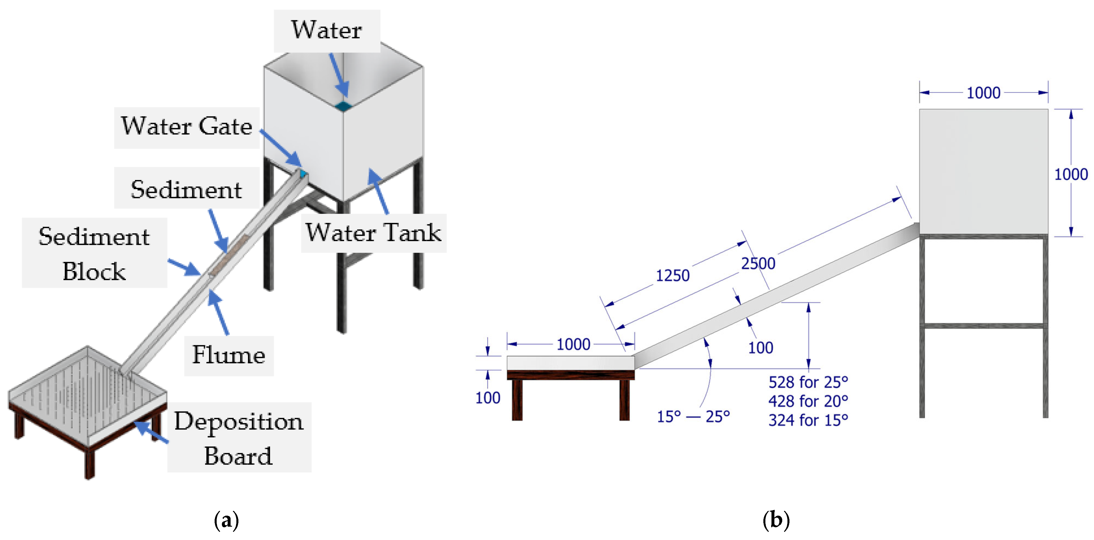
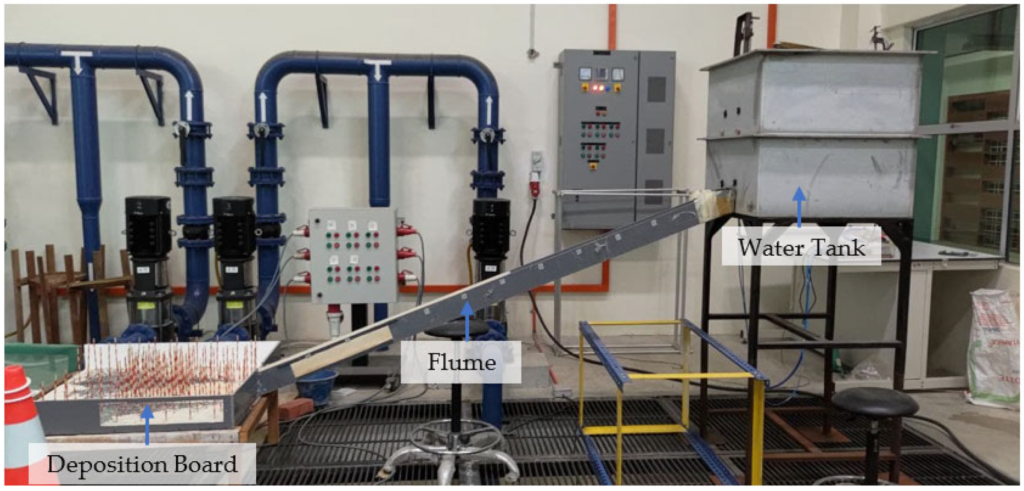
2.1. Physical Model Test
2.2. Physical Model Configuration
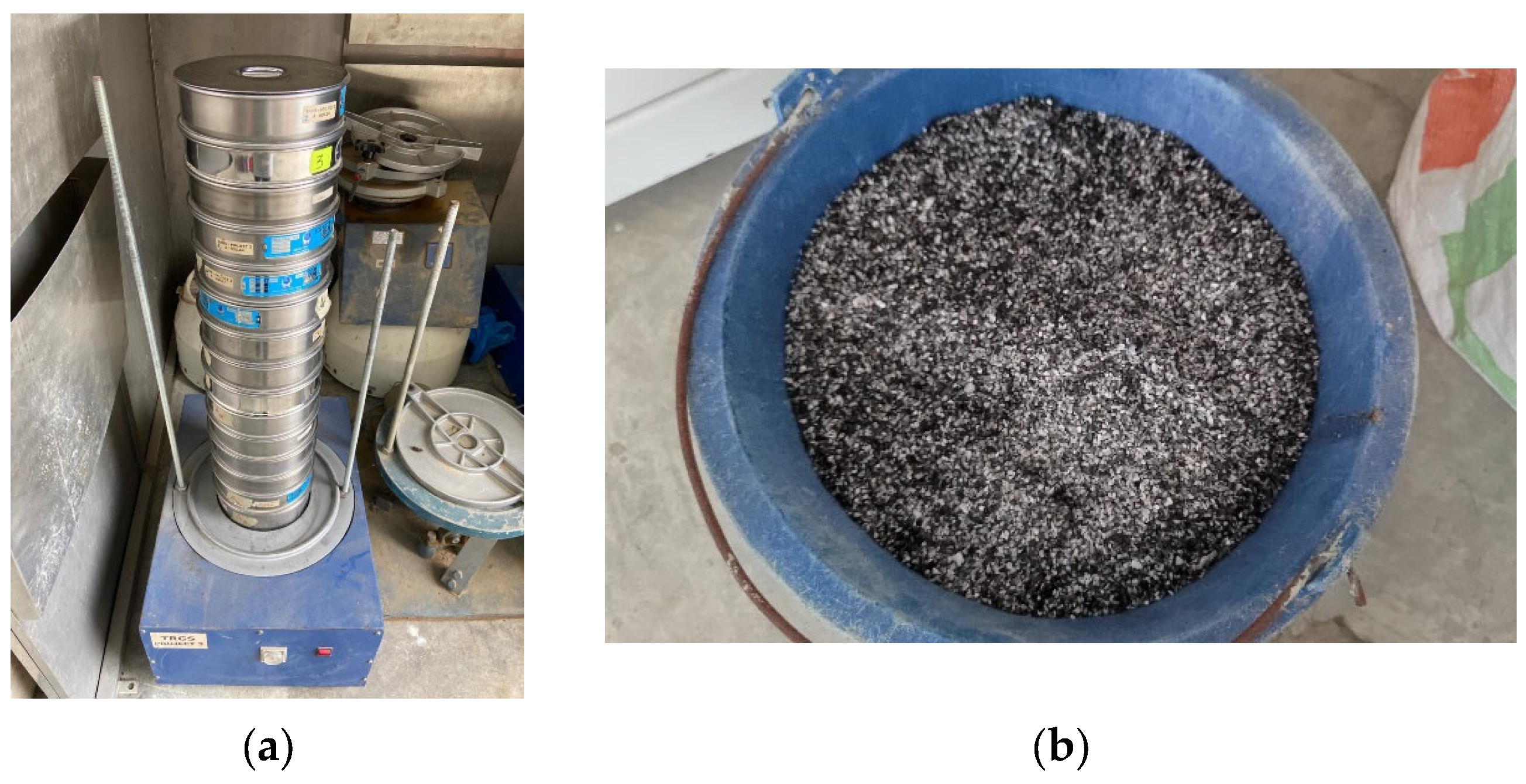
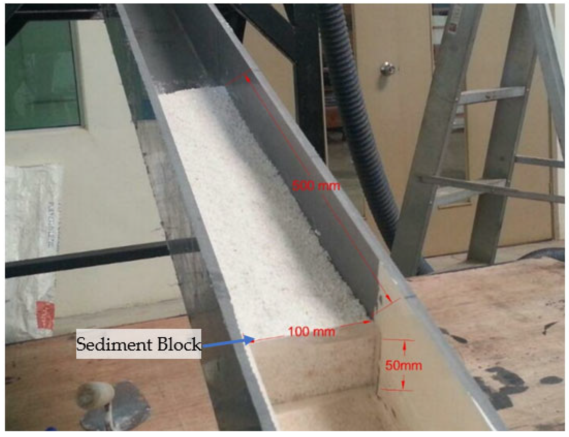
2.2.1. Sediment Particle and Preparation
2.2.2. Water Tank
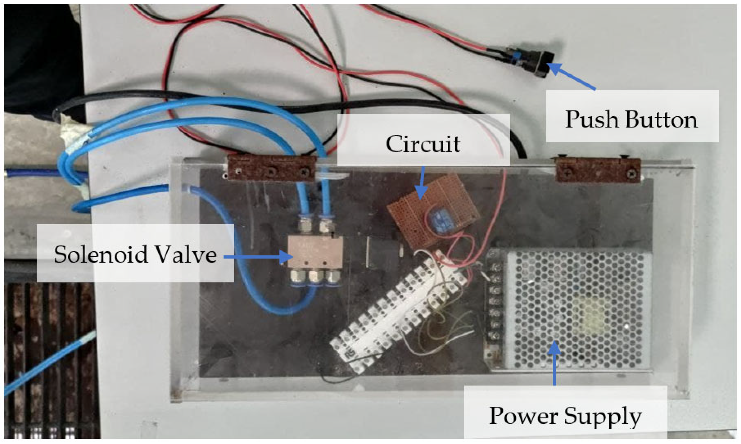
2.2.3. Water Gate Opening
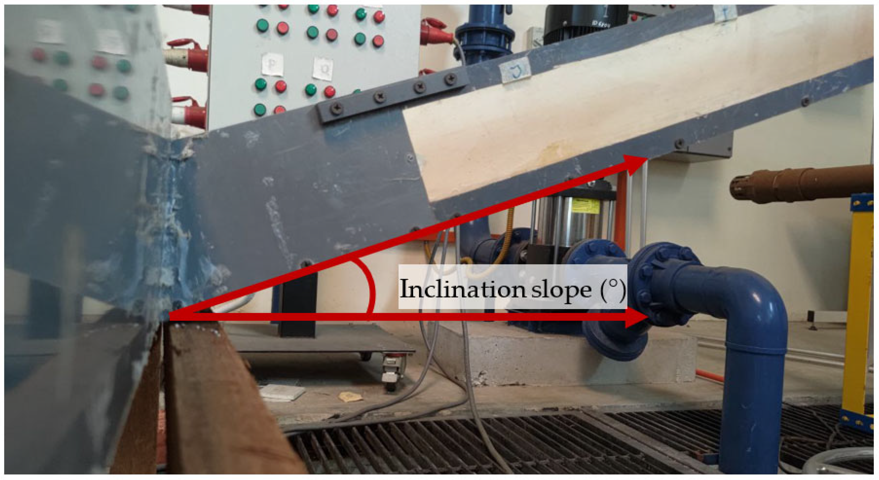
2.2.4. Inclination of Flume
2.2.5. Deposition Board
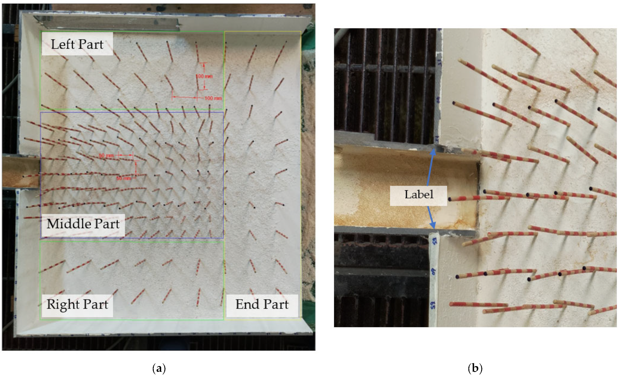
2.3. Data Collection
2.3.1. Shape and Thickness
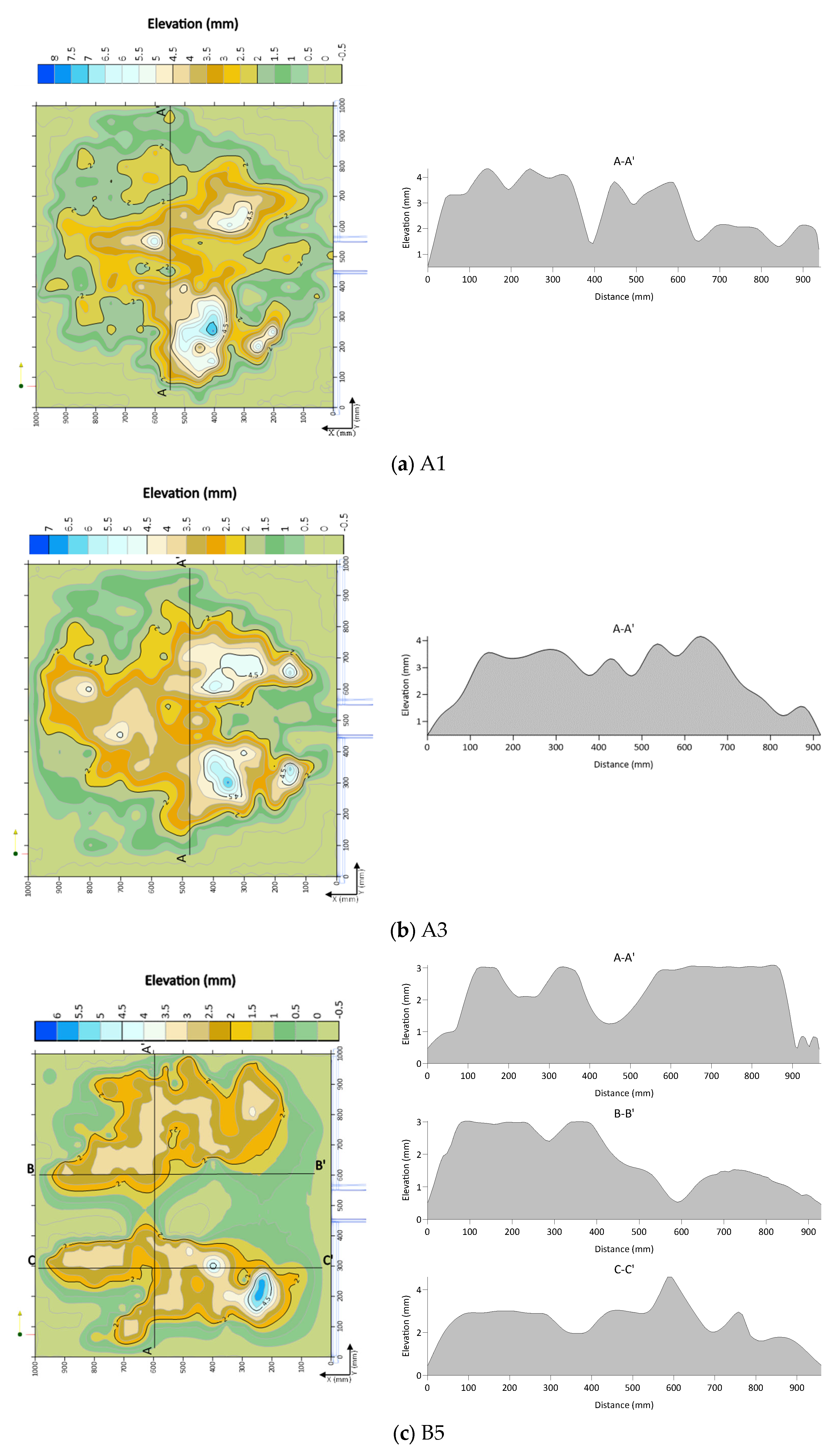
2.3.2. Contour Sketch and Visualize
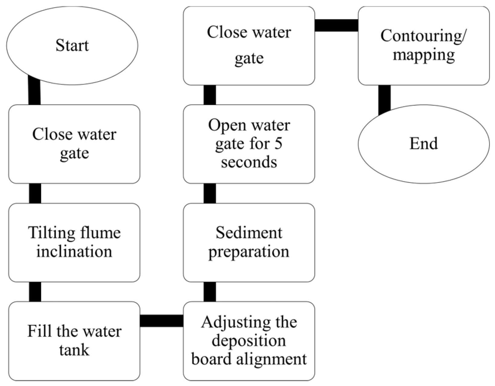
2.4. Test Procedure
3. Results and Discussions
3.1. Deposition Observation
3.2. Statistical Analysis
4. Conclusions
Author Contributions
Funding
Institutional Review Board Statement
Informed Consent Statement
Data Availability Statement
Acknowledgments
Conflicts of Interest
References
- Takahashi, T. A Review of Japanese Debris Flow Research. Int. J. Eros. Control Eng. 2013, 2, 1–14. [Google Scholar] [CrossRef]
- Zhou, G.D.; Law, R.P.H.; Ng, C.W.W. The mechanisms of debris flow: A preliminary study. In Proceedings of the 17th International Conference on Soil Mechanics and Geotechnical Engineering: The Academia and Practice of Geotechnical Engineering, Alexandria, Egypt, 5–9 October 2009; Volume 2, pp. 1570–1573. [Google Scholar]
- Mohd Arif Zainol, M.R.R.; AWahab, M.K. Hydraulic Physical Model of Debris Flow for Malaysia Case Study. In Proceedings of the IOP Conference Series: Materials Science and Engineering, Iasi, Romania, 17–18 May 2018; Institute of Physics Publishing: Bristol, UK, 2018; Volume 374. [Google Scholar]
- Tiranti, D.; Crema, S.; Cavalli, M.; Deangeli, C. An Integrated Study to Evaluate Debris Flow Hazard in Alpine Environment. Front. Earth Sci. 2018, 6, 60. [Google Scholar] [CrossRef]
- Muhammad, N.S.; Julien, P.Y.; Salas, J.D. Probability Structure and Return Period of Multiday Monsoon Rainfall. J. Hydrol. Eng. 2016, 21, 0401548. [Google Scholar] [CrossRef]
- Rahman, H.A.; Mapjabil, J. Landslides Disaster in Malaysia: An Overview. Health Environ. J. 2017, 8, 58–71. [Google Scholar]
- Joe, E., Jr.; Tongkul, F.; Roslee, R. Engineering Properties of Debris Flow Material at Bundu Tuhan, Ranau, Sabah, Malaysia. Pak. J. Geol. 2018, 2, 22–26. [Google Scholar] [CrossRef]
- Kasim, N.; Taib, K.A.; Mukhlisin, M.; Kasa, A. Triggering Mechanism and Characteristic of Debris Flow in Peninsular Malaysia. Am. J. Eng. Res. 2016, 5, 112–119. [Google Scholar]
- Liu, K.F.; Huang, M.C. Numerical simulation of debris flows. In Proceedings of the International Conference on Offshore Mechanics and Arctic Engineering—OMAE, Honolulu, HI, USA, 31 May–5 June 2009; Volume 6, pp. 375–382. [Google Scholar]
- Chang, T.C.; Wang, Z.Y.; Chien, Y.H. Hazard assessment model for debris flow prediction. Environ. Earth Sci. 2010, 60, 1619–1630. [Google Scholar] [CrossRef]
- Li, M.L.; Jiang, Y.J.; Yang, T.; Huang, Q.B.; Qiao, J.P.; Yang, Z.J. Early warning model for slope debris flow initiation. J. Mt. Sci. 2018, 15, 1342–1353. [Google Scholar] [CrossRef]
- Vargas-Cuervo, G.; Rotigliano, E.; Conoscenti, C. Prediction of debris-avalanches and -flows triggered by a tropical storm by using a stochastic approach: An application to the events occurred in Mocoa (Colombia) on 1 April 2017. Geomorphology 2019, 339, 31–43. [Google Scholar] [CrossRef]
- Zhou, J.W.; Cui, P.; Yang, X.G.; Su, Z.M.; Guo, X.J. Debris flows introduced in landslide deposits under rainfall conditions: The case of Wenjiagou gully. J. Mt. Sci. 2013, 10, 249–260. [Google Scholar] [CrossRef]
- Chen, S.C.; Wu, C.Y. Debris flow disaster prevention and mitigation of non-structural strategies in Taiwan. J. Mt. Sci. 2014, 11, 308–322. [Google Scholar] [CrossRef]
- Lay, U.S.; Pradhan, B. Identification of Debris Flow Initiation Zones Using Topographic Model and Airborne Laser Scanning Data. In Lecture Notes in Civil Engineering, Proceedings of the GCEC 2017: The 1st Global Civil Engineering Conference 1, Kuala Lumpur, Malaysia, 25–28 July; Pradhan, B., Ed.; Springer: Singapore, 2019; Volume 9. [Google Scholar]
- Pradhan, B.; Bakar, S.B.A. Debris Flow Source Identification in Tropical Dense Forest Using Airborne Laser Scanning Data and Flow-R Model. In Laser Scanning Applications in Landslide Assessment; Pradhan, B., Ed.; Springer: New York, NY, USA, 2017; pp. 85–112. [Google Scholar]
- Borga, M.; Stoffel, M.; Marchi, L.; Marra, F.; Jakob, M. Hydrogeomorphic response to extreme rainfall in headwater systems: Flash floods and debris flows. J. Hydrol. 2014, 518, 194–205. [Google Scholar] [CrossRef]
- Liu, X.; Wang, F.; Nawnit, K.; Lv, X.; Wang, S. Experimental study on debris flow initiation. Bull. Eng. Geol. Env. 2020, 79, 1565–1580. [Google Scholar] [CrossRef]
- Zhuang, J.Q.; Cui, P.; Peng, J.B.; Hu, K.H.; Iqbal, J. Initiation process of debris flows on different slopes due to surface flow and trigger-specific strategies for mitigating post-earthquake in old Beichuan County, China. Environ. Earth Sci. 2013, 68, 1391–1403. [Google Scholar] [CrossRef]
- Jeong, S.; Lee, J.; Song, C.G.; Lee, S.O. Propagation characteristics of debris flows considering entrainment effect. Int. J. Eng. Technol. 2018, 7, 122–128. [Google Scholar] [CrossRef]
- Rickenmann, D.; Scheidl, C. Debris-Flow Runout and Deposition on the Fan. In Dating Torrential Processes on Fans and Cones; Springer: Dordrecht, The Netherlands, 2012; Volume 47, pp. 75–93. [Google Scholar]
- Wang, W.; Chen, G.; Han, Z.; Zhou, S.; Zhang, H.; Jing, P. 3D numerical simulation of debris-flow motion using SPH method incorporating non-Newtonian fluid behavior. Nat. Hazards 2016, 81, 1981–1998. [Google Scholar] [CrossRef]
- Talling, P.J.; Wynn, R.B.; Masson, D.G.; Frenz, M.; Cronin, B.T.; Schiebel, R.; Amy, L.A. Onset of submarine debris flow deposition far from original giant landslide. Nature 2007, 450, 541–544. [Google Scholar] [CrossRef]
- Bouchut, F.; Vilotte, J.P.; Lajeunesse, E.; Aubertin, A.; Pirulli, M. On the use of Saint Venant equations to simulate the spreading of a granular mass. J. Geophys. Res. Solid Earth 2005, 110, 1–17. [Google Scholar]
- Jakob, M.; Stein, D.; Ulmi, M. Vulnerability of buildings to debris flow impact. Nat. Hazards 2012, 60, 241–261. [Google Scholar] [CrossRef]
- Stancanelli, L.M.; Musumeci, R.E. Geometrical characterization of sediment deposits at the confluence of mountain streams. Water 2018, 10, 401. [Google Scholar] [CrossRef]
- Liu, J.; Nakatani, K.; Mizuyama, T. Effect assessment of debris flow mitigation works based on numerical simulation by using Kanako 2D. Landslides 2013, 10, 161–173. [Google Scholar] [CrossRef]
- Calhoun, N.C.; Clague, J.J. Distinguishing between debris flows and hyperconcentrated flows: An example from the eastern Swiss Alps. Earth Surf. Process. Landf. 2018, 43, 1280–1294. [Google Scholar] [CrossRef]
- Yamashiki, Y.; Rozainy, M.A.Z.M.R.; Matsumoto, T.; Takahashi, T.; Takara, K. Particle Routing Segregation of Debris Flow Mechanisms Near the Erodible Bed. APCBEE Procedia 2013, 5, 527–534. [Google Scholar] [CrossRef]
- Tan, B.K. Environmental Geology of Limestone in Malaysia. IGCP 2002, 448, 54–67. [Google Scholar]
- Turnbull, B.; Bowman, E.T.; McElwaine, J.N. Debris flows: Experiments and modelling. Comptes Rendus Phys. 2015, 16, 86–96. [Google Scholar] [CrossRef]
- Chang, T.C.; Chien, Y.H. The application of genetic algorithm in debris flows prediction. Environ. Geol. 2007, 53, 339–347. [Google Scholar] [CrossRef]
- Lin, D.G.; Hsu, S.Y.; Chang, K.T. Numerical simulations of flow motion and deposition characteristics of granular debris flows. Nat. Hazards 2009, 50, 623–650. [Google Scholar] [CrossRef]
- Reid, M.E.; Iverson, R.M.; Logan, M.; Lahusen, R.G.; Godt, J.W.; Griswold, J.P. Entrainment of bed sediment by debris flows: Results from large-scale experiments. Ital. J. Eng. Geol. Environ. 2011, 367–374. [Google Scholar]
- Bettella, F.; Michelini, T.; D’Agostino, V.; Bischetti, G.B. The ability of tree stems to intercept debris flows in forested fan areas: A laboratory modelling study. J. Agric. Eng. 2018, 49, 42–51. [Google Scholar] [CrossRef]
- Maris, F.; Potouridis, S.; Angelidis, P. Kriging Interpolation Method for Estimation of Continuous Spatial Distribution of Precipitation in Cyprus. Br. J. Appl. Sci. Technol. 2013, 3, 1286–1300. [Google Scholar] [CrossRef]
- Marschallinger, R. Interface programs to enable full 3-D geological modeling with a combination of AutoCAD and SURFER. Comput. Geosci. 1991, 17, 1383–1394. [Google Scholar] [CrossRef]
- Yang, C.-S.; Kao, S.-P.; Lee, F.-B.; Hung, P.-S. Twelve different interpolation methods: A case study of Surfer 8.0. Proc. XXth ISPRS Congr. 2004, 35, 778–785. [Google Scholar]
- Chang, H.; Ryou, K.; Lee, H. Debris flow characteristics in flume experiments considering berm installation. Applied Sciences 2021, 11, 2336. [Google Scholar] [CrossRef]
- Luna, B.Q.; Remaître, A.; van Asch, T.W.J.; Malet, J.P.; van Westen, C.J. Analysis of debris flow behavior with a one dimensional run-out model incorporating entrainment. Eng. Geol. 2012, 128, 63–75. [Google Scholar] [CrossRef]
- Song, E.; Oh, M.S.; Billard, L.; Moss, A.; Pesti, G.M. A statistical analysis of nonlinear regression models for different treatments for layers. Poult. Sci. 2002, 101, 102004. [Google Scholar] [CrossRef]


| Case Study | Flume Degree (°) | Water Level (mm) | Gate Opening |
|---|---|---|---|
| A1 | 15 | 120 | Half |
| A2 | 15 | 120 | Full |
| A3 | 15 | 150 | Half |
| A4 | 15 | 150 | Full |
| B5 | 20 | 120 | Half |
| B6 | 20 | 120 | Full |
| B7 | 20 | 150 | Half |
| B8 | 20 | 150 | Full |
| C9 | 25 | 120 | Half |
| C10 | 25 | 120 | Full |
| C11 | 25 | 150 | Half |
| C12 | 25 | 150 | Full |
| Type | Remarks |
|---|---|
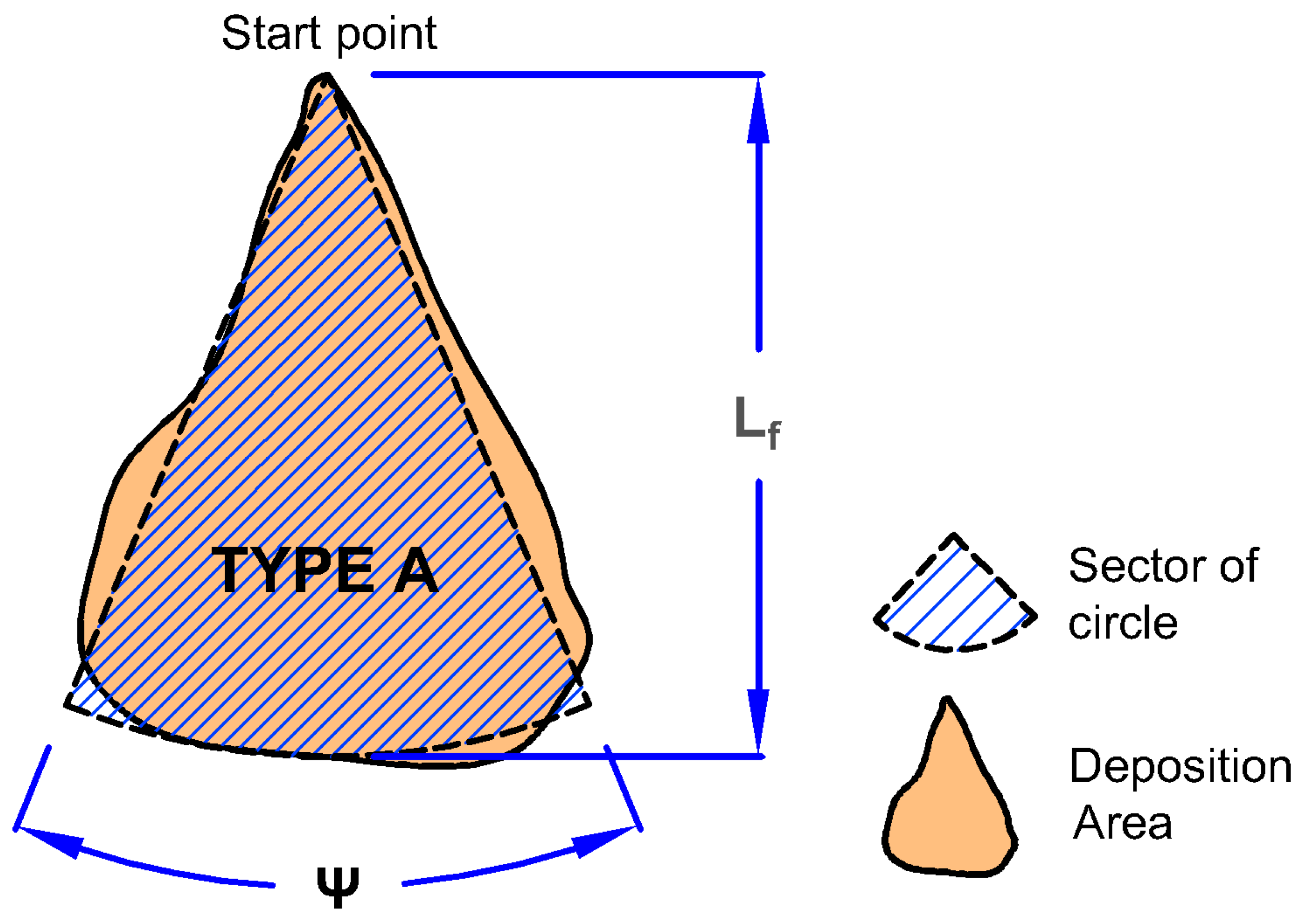
| A | Represents an ideal shape for uniform runout patterns with no obstructions or distinct channels on the fan affect deposition. Typically, the topography causes the material to rise over the channel and begin to spread over the fan. |
| B1 | Obstructions such as structures or mitigation measures in the lower part of the deposition region affect the deposition pattern. |
| B2 | |
| C1 | Linear structures crossing the deposition zone, such as roads, railway tracks, or receiving streams that caused a pronounced lateral spreading in the lower part of the deposition region. |
| C2 | |
| D |
| Case Study | Total Volume of Deposited Sediment (mm3) | Total Volume of Sediment Retained in Strainer (mm3) | Planar Area (mm2) | Surface Area (mm2) | Aperture Angle (°) | Highest Point (mm) | Percentage Particle on Deposition Board (%) | Type of Pattern | Lfpred [21] (mm) |
|---|---|---|---|---|---|---|---|---|---|
| A1 | 1.677518 × 10³ | 2498.322 × 103 | 536.79 × 10³ | 537.07 × 10³ | 90.19 | 7.5 | 53.68% | A | 884.87 |
| A2 | 1.508610 × 10³ | 2498.491 × 103 | 436.93 × 10³ | 437.13 × 10³ | 86.63 | 6.5 | 43.69% | A | 902.50 |
| A3 | 1.656639 × 10³ | 2498.343 × 103 | 488.42 × 10³ | 488.65 × 10³ | 81.83 | 6.5 | 48.84% | A | 928.07 |
| A4 | 1.544908 × 10³ | 2498.455 × 103 | 402.34 × 10³ | 402.61 × 10³ | 67.87 | 7.5 | 40.23% | A | 1017.15 |
| B5 | 1.497587 × 10³ | 2498.502 × 103 | 461.38 × 10³ | 461.57 × 10³ | 124.88 | 5.5 | 46.14% | A | 754.44 |
| B6 | 1.730672 × 10³ | 2498.269 × 103 | 447.06 × 10³ | 447.57 × 10³ | 98.87 | 7 | 44.71% | A | 845.91 |
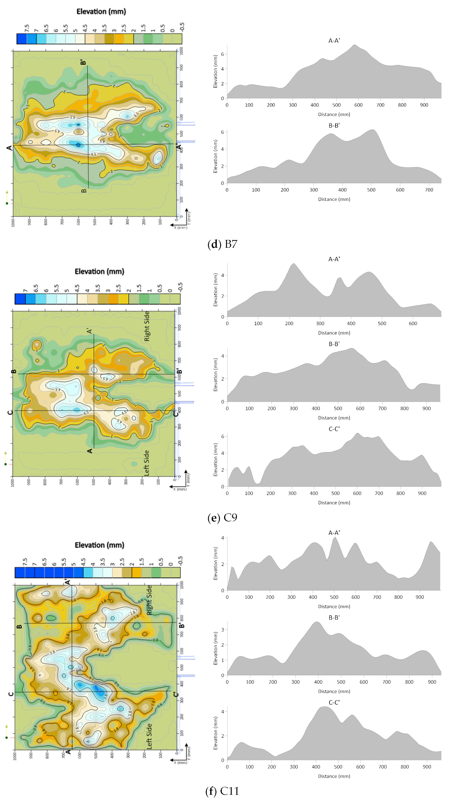
| B7 | 1.54 × 10³ | 2498.460 × 103 | 415.86 × 10³ | 416.17 × 10³ | 85.46 | 7 | 41.59% | A | 908.54 |
| B8 | 1.048050 × 10³ | 2498.951 × 103 | 290.03 × 10³ | 290.33 × 10³ | 84.00 | 6.5 | 29.00% | A | 916.24 |
| C9 | 1.312914 × 10³ | 2498.687 × 103 | 367.62 × 10³ | 367.87 × 10³ | 86.52 | 6.5 | 36.75% | A | 903.07 |
| C10 | 1.251489 × 10³ | 2498.748 × 103 | 321.46 × 10³ | 321.93 × 10³ | 73.17 | 11 | 32.15% | A | 980.36 |
| C11 | 1.377437 × 10³ | 2498.622 × 103 | 485.07 × 10³ | 485.23 × 10³ | 102.45 | 4.4 | 48.51% | A | 831.30 |
| C12 | 1.179189 × 10³ | 2498.820 × 103 | 298.70 × 10³ | 299.02 × 10³ | 65.86 | 7 | 29.87% | A | 1032.24 |
| θd (°) | Vw (mm3) | VT (mm3) | Vout (mm3) | PA (mm2) | SA (mm2) | Ψ (°) | HP (mm) | PB (%) | |
|---|---|---|---|---|---|---|---|---|---|
| θd (°) | 1 | ||||||||
| Vw (mm3) | 0.000 | 1 | |||||||
| VT (mm3) | −0.637 * | −0.260 | 1 | ||||||
| Vout (mm3) | −0.005 | 0.783 ** | −0.315 | 1 | |||||
| PA (mm2) | −0.527 | −0.210 | 0.844 ** | −0.410 | 1 | ||||
| SA (mm2) | −0.527 | −0.210 | 0.844 ** | −0.411 | 1.000 ** | 1 | |||
| Ψ (°) | 0.302 | −0.285 | −0.078 | −0.305 | 0.130 | 0.129 | 1 | ||
| HP (mm) | −0.248 | 0.107 | −0.308 | 0.107 | −0.418 | −0.418 | −0.565 | 1 | |
| PB (%) | −0.527 | −0.210 | 0.844 ** | −0.410 | 1.000 ** | 1.000 ** | 0.129 | −0.418 | 1 |
| θd (°) | Vw (mm3) | ||||||
|---|---|---|---|---|---|---|---|
| Variable | Regression Type | R2 (%) | S | Equation | R2 (%) | S | Equation |
| VT (mm3) | Linear | 40.6 | 171.288 | VT = 2077 − 31.67θd | 6.75 | 214.616 | VT = 1918 − 3.514Vw |
| Quadratic | 40.7 | 180.357 | VT = 1840 − 69θd − 0.620θd2 | N/A | N/A | N/A | |
| Nonlinear | N/A | 180.835 | VT = exp(−0.0218546θd)/(0.000449157 + 1.72044 × 10⁻¹²θd) | N/A | 1157.87 | VT = exp(−0.0172781Vw)/(−1.1024 + 0.00918734Vw) | |
| Vout (mm3) | Linear | 0.0 | 222.246 | Vout = 2,498,562 − 0.27θd | 138.18 | 61.34 | Vout = 2,497,126 + 10.59Vw |
| Quadratic | 0.01 | 234.261 | Vout = 2,498,510 + 5.2θd − 0.136θd2 | N/A | N/A | N/A | |
| Nonlinear | N/A | 234.268 | Vout = exp(−1.0799 × 10⁻⁷θd)/(4.0023 × 10−7 − 3.31555 × 10⁻¹⁶θd) | N/A | 2,040,192 | Vout = exp(−0.0296687Vw)/(−1.10221 + 0.00918512Vw) | |
| PA (mm2) | Linear | 27.78 | 70,606.7 | PA = 608,453 − 9791θd | 4.4 | 81,234.5 | PA = 555,753 − 1060Vw |
| Quadratic | 28.49 | 74,057.8 | PA = 816,737 – 31,525θd + 543θd2 | N/A | N/A | N/A | |
| Nonlinear | N/A | 74,057.8 | PA = exp(0.0223781θd)/(3.74916 × 10−7 + 1.7508 × 10⁻⁷θd) | N/A | 335,061 | PA = exp(−0.0277149Vw)/(−1.10245 + 0.00918709Vw) | |
| SA (mm2) | Linear | 27.77 | 70,574.4 | SA = 608,634 − 9785θd | 4.41 | 81,187.1 | SA = 556,277 − 1062Vw |
| Quadratic | 28.48 | 74,026.5 | SA = 816,075 − 31,431θd + 541θd2 | N/A | N/A | N/A | |
| Nonlinear | N/A | 74,026.5 | SA = exp(0.0222817θd)/(3.83081 × 10−7 + 1.74142 × 10⁻⁷θd) | N/A | 335,257 | SA = exp(−0.0276883Vw)/(−1.10245 + 0.00918709Vw) | |
| Ψ (°) | Linear | 9.14 | 16.1373 | Ψ = 64.42 + 1.145θd | 8.11 | 16.2287 | Ψ = 126.9 − 0.2934Vw |
| Quadratic | 29.92 | 14.9388 | Ψ = 293.6 − 22.77θd + 0.5978θd2 | N/A | N/A | N/A | |
| Nonlinear | N/A | 14.9388 | Ψ = exp(0.134118θd)/(−0.221576 + 0.0205293θd) | N/A | 17.1065 | Ψ = exp(0.0274097Vw)/(−1.48245 + 0.0147908Vw) | |
Disclaimer/Publisher’s Note: The statements, opinions and data contained in all publications are solely those of the individual author(s) and contributor(s) and not of MDPI and/or the editor(s). MDPI and/or the editor(s) disclaim responsibility for any injury to people or property resulting from any ideas, methods, instructions or products referred to in the content. |
© 2023 by the authors. Licensee MDPI, Basel, Switzerland. This article is an open access article distributed under the terms and conditions of the Creative Commons Attribution (CC BY) license (https://creativecommons.org/licenses/by/4.0/).
Share and Cite
A.Wahab, M.K.; Mohd Arif Zainol, M.R.R.; Ikhsan, J.; Zawawi, M.H.; Abas, M.A.; Mohamed Noor, N.; Abdul Razak, N.; Sholichin, M. Assessment of Debris Flow Impact Based on Experimental Analysis along a Deposition Area. Sustainability 2023, 15, 13132. https://doi.org/10.3390/su151713132
A.Wahab MK, Mohd Arif Zainol MRR, Ikhsan J, Zawawi MH, Abas MA, Mohamed Noor N, Abdul Razak N, Sholichin M. Assessment of Debris Flow Impact Based on Experimental Analysis along a Deposition Area. Sustainability. 2023; 15(17):13132. https://doi.org/10.3390/su151713132
Chicago/Turabian StyleA.Wahab, Muhammad Khairi, Mohd Remy Rozainy Mohd Arif Zainol, Jazaul Ikhsan, Mohd Hafiz Zawawi, Mohamad Aizat Abas, Norazian Mohamed Noor, Norizham Abdul Razak, and Moh Sholichin. 2023. "Assessment of Debris Flow Impact Based on Experimental Analysis along a Deposition Area" Sustainability 15, no. 17: 13132. https://doi.org/10.3390/su151713132
APA StyleA.Wahab, M. K., Mohd Arif Zainol, M. R. R., Ikhsan, J., Zawawi, M. H., Abas, M. A., Mohamed Noor, N., Abdul Razak, N., & Sholichin, M. (2023). Assessment of Debris Flow Impact Based on Experimental Analysis along a Deposition Area. Sustainability, 15(17), 13132. https://doi.org/10.3390/su151713132