Analysis of Factors Influencing the Severity of Vehicle-to-Vehicle Accidents Considering the Built Environment: An Interpretable Machine Learning Model

Abstract

Understanding the causes of traffic road accidents is crucial; however, as data collection is conducted by traffic police, accident-related environmental information is not available. To fill this gap, we collect information on the built environment within R = 500 m of the accident site; model the factors influencing accident severity in Shenyang, China, from 2018 to 2020 using the Random Forest algorithm; and use the SHapley Additive exPlanation method to interpret the underlying driving forces. We initially integrate five indicators of the built environment with 18 characteristics, including human and vehicle at-fault characters, infrastructure, time, climate, and land use attributes. Our results show that road type, urban/rural, season, and speed limit in the first 10 factors have a significant positive effect on accident severity; density of commercial-POI in the first 10 factors has a significant negative effect. Factors such as urban/rural and road type, commercial and vehicle type, road type, and season have significant effects on accident severity through an interactive mechanism. These findings provide important information for improving road safety.

1. Introduction

In recent years, the analysis of road traffic crashes has emerged as a critical area of research in sustainable urban development, primarily due to the severe consequences of such crashes, which result in significant human and property losses. The World Health Organization reports that road traffic accidents account for approximately 1.35 million deaths yearly [1]. Consequently, identifying effective strategies to mitigate fatalities from road traffic accidents has become a shared objective among scholars and policymakers.

Efforts to reduce deaths in road traffic accidents can be broadly categorized into two areas of focus: decreasing the frequency of accidents and minimizing the severity of accidents [2]. Studies investigating the frequency of road traffic accidents emphasize the typical characteristics of accident-prone locations [3], while research examining the severity of road traffic accidents tends to explore the mechanisms through which various key factors influence accident severity [4,5].

In constructing the set of influencing factors, previous research has predominantly relied on traffic police-reported data and has focused on driver characteristics [6]. However, the built environment also considerably impacts road traffic accidents [7]. Researchers discovered early in the exploration process that the objective environment has an unavoidable influence on accidents. Early urban planning attached importance to incremental development, and problems existed in land use, job–housing balance, and traffic density, which affected residents’ travel patterns. Moreover, residents’ traffic demand and supply conflicts were significant, which to some extent affected traffic safety. Scholars have found through numerous studies that the probability and severity of urban traffic accidents are closely related to the built environment and that the built environment directly affects regional traffic flow, speed, and traffic conflicts. Therefore, adding the influence of the built environment to accident analysis can obtain a more principled analysis of accidents than using only police survey data.

While identifying key influencing factors, mathematical statistics or machine learning methods are commonly employed. Mathematical statistics have stronger model interpretability. Still, machine learning methods can explore more complex relationships between the independent and dependent variables [8]. In a study by Ahmed et al. [9], six different machine learning algorithms, namely Random Forest (RF), Decision Jungle (DJ), Adaptive Boost (AdaBoost), Extreme Gradient Boost (XGBoost), Light Gradient Boost Machine (LGBM), and Classification Boost (CatBoost), were used to analyze road accidents in New Zealand from 2016 to 2020, and they showed that RF has the best prediction results. Therefore, in this study, we utilize the Random Forest (RF) algorithm to explore key influencing factors, including considering the surrounding environmental features of the accident locations. Furthermore, we apply the SHapley Additive exPlanation (SHAP) method [10] to complement the inherent interpretability shortcomings of machine learning methods, facilitating a deeper exploration of the impact trends on crucial determinants of crash severity.

The objective of this paper is to integrate macroscopic built environment data with police-reported data. We aim to explore the role of various factors in accidents from the perspective of the at-fault party, especially examining if certain built environment factors lead to fatal outcomes. Additionally, we will investigate the impact of dual-factor interactions on fatal and non-fatal accidents to provide targeted theoretical support and policy recommendations. The remainder of this paper organized as follows: Section 2 is a summary of the past research, Section 3 presents an overview of the data, Section 4 introduces the proposed methodological framework, Section 5 presents the results, and Section 6 discusses the implications those results have for policy making regarding pedestrian safety.

2. Literature Review

In exploring determinants affecting the severity of road traffic accidents, the academic literature primarily emphasizes six key dimensions: human factors, vehicle factors, road characteristics, crash characteristics, time, and environmental conditions [11]. Among them, human and vehicle factors include aspects such as driver’s age [12], gender [13], driving experience [14], and vehicle type [15]; road characteristics involve elements such as the physical isolation of the road [16], road type [17], and other variables; crash characteristics include factors such as accident reason [18], cross-sectional location [19], whether it occurred at an intersection [20], and other elements; time and environmental conditions include variables such as seasonality [21], weather [22], climatic factors [23], and other variables. The relationship between traffic accidents and the built environment has been proposed since the last century. Researchers have been trying to discover the contributing factors behind accidents through micro- and macro-level studies. Ding et al. [24] found a significant nonlinear relationship between some built environment factors and pedestrian crash frequency. Ewing et al. [25] found two conclusions that defy previous knowledge: dense urban traffic environments are safer than suburban areas, and unforgiving design treatments may improve road safety. The probability and severity of urban traffic accidents are closely related to the built environment, which affects regional traffic flows, speeds, and traffic conflicts. Although human causes are the primary influence on accident occurrence [26], various studies have shown that there are still unidentified influences. Scholars have found that accident rates are reduced around schools, while commercial areas positively impact accidents [27]. The intensity of land use impacts accidents, thus leading to the possible influence of the built environment. The factors that may affect the accident are derived from the built environment. In addition, Lee et al. [28] also found the influence of the built environment on different age groups of pedestrians, and Merlin et al. [29] focused on the relationship between the characteristics of the built environment and crash rates in smaller geographical units. Accident analysis that considers the built environment objectively explores existing buildings from a microscopic perspective and considers the problem more comprehensively.

Over the years, mathematical and statistical methods have remained a standard part of analyzing factors influencing traffic accidents. Several researchers have employed these methods to gain insights into different aspects of traffic accidents. Nam et al. (2000) conducted a statistical analysis of many factors impacting incident duration [30]. Huang et al. (2008) implemented a binomial logistic model to assess the severity of driver injuries at intersections in traffic accidents [31]. In a study on significant factors affecting crash injury severity at public highway–railroad-grade crossings, Haleem and Gan (2015) proposed using a mixed logit model [32]. More recently, Wang et al. (2021) developed an evaluation system based on crash characteristics and identified key influencing factors using a multinomial logit model [33]. Mathematical statistical methods typically provide detailed results for judging factor significance; however, since they are generally employed when the model has been verified as feasible, there are limitations on the factors that can be included in the statistical calculations.

In recent years, machine learning models have emerged as a popular approach for identifying crucial factors that influence traffic accidents. Various studies have employed different machine learning algorithms to predict and analyze traffic accident data. For instance, Xu and Luo (2021) developed a prediction and early warning model using the Random Forest algorithm, which demonstrated good predictive performance for unsafe acts [34]. Yang et al. (2022) applied methods such as the Random Forest algorithm and Bayesian logistics regression to identify crash precursors for each type of highway area [35]. Das A et al. applied conditional inference forests to identify risk factors for collision severity for clusters of different arterial corridor lengths [36]. Similarly, Wen et al. (2021) applied the Shapley Additive exPlanation (SHAP) approach to interpret the outputs of machine learning methods when analyzing risk factors associated with road segment crashes [37], the research found that the RF method is efficient in situations where potential variables have complicated relationships, such as those impacting crash severity. Chang et al. (2022) investigated the nonlinear relationship between pedestrian fatalities and related factors using the XGBoost model, with the results being interpreted through the SHAP method [38]. Yang et al. (2022) used the same approach to conduct an exploratory analysis of the factors in freight-truck-related crashes [39]. Wang et al. (2022) sought to identify the causes of varying levels of delay in metropolitan and non-metropolitan areas using improved the Random Forest and LightGBM algorithms [40]. In a study by Shakil Ahmed et al. [9], six different machine learning algorithms, Random Forest (RF), Decision Jungle (DJ), Adaptive Boost (AdaBoost), Extreme Gradient Boost (XGBoost), Light Gradient Booster Machine (LGBM), and Classification Boost (CatBoost), were used to New Zealand for the period 2016 to 2020 road accident data for analysis and prediction. The comparison results show that RF prediction is the best.

While machine learning methods have certain limitations, such as reduced explanatory power, which biggest drawback is cannot explain the cause–effect relationship, but can only be used to explain the correlation between variables, their flexible data requirements make them suitable for considering a wide range of influencing factors. In addition, the application of the SHAP method can also circumvent the limitations of machine learning methods to provide valuable insights into the underlying factors influencing traffic accidents. Overall, this study employs a machine learning method in conjunction with SHAP to analyze factors that impact the severity of road traffic accidents.

3. Data

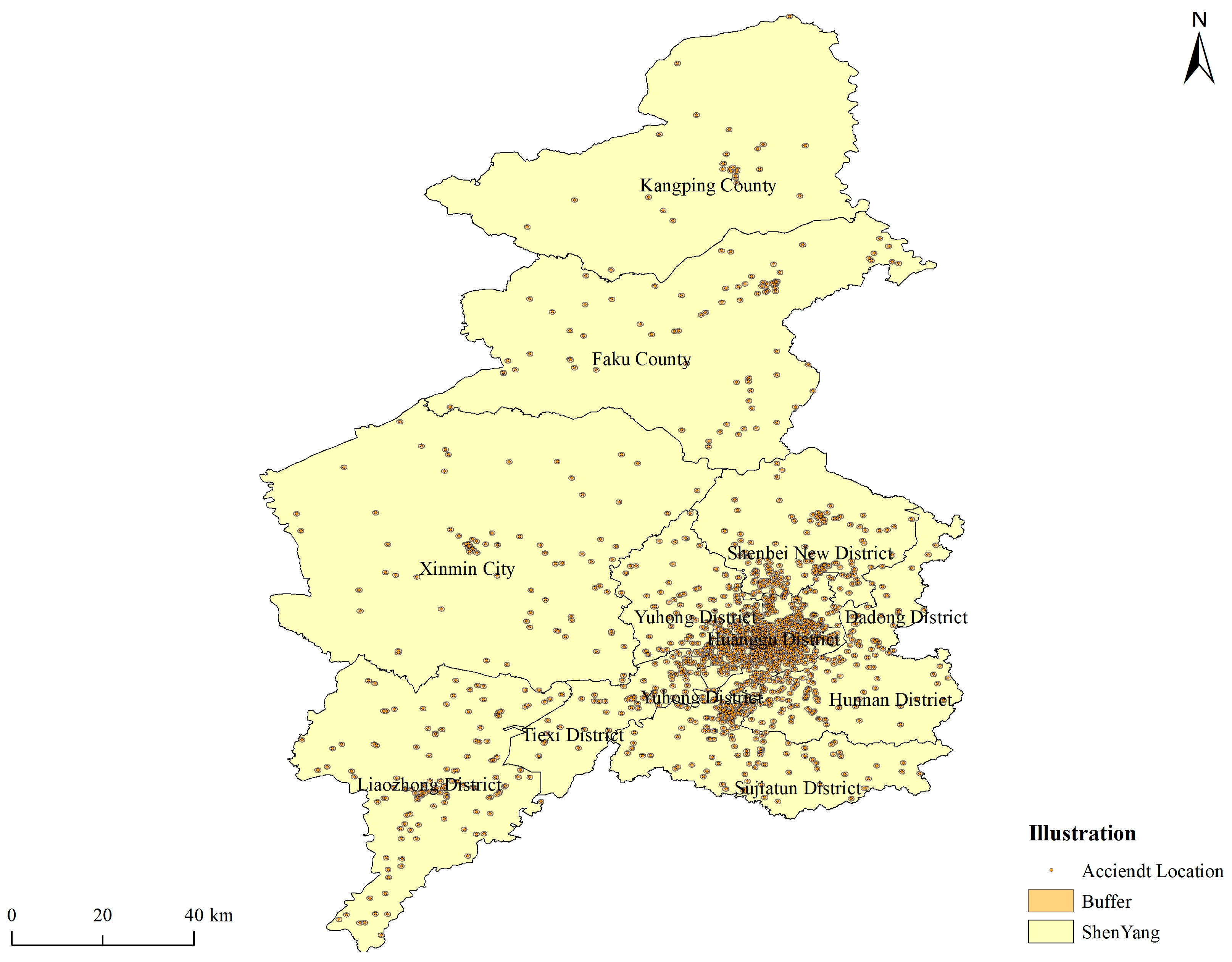
3.1. Data Resource and Processing

This research is conducted based on the traffic accident data from 2018 to 2020 in Shenyang, Liaoning Province, China. The accident characteristics data reported by the traffic police only pointed out the specific address of each accident, we used technical means to convert the text into latitude and longitude under the WGS84 coordinate system.

The following preliminary screening of samples is performed considering the demand of the Random Forest model for sample size and the availability of data sources:

(1)

Data containing pedestrians and collision data of single vehicles were excluded; data on crash between motor vehicles and motor vehicles, non-motor vehicles and motor vehicles, and non-motor vehicles and non-motor vehicles were selected;

(2)

Extracted data on driver accidents with equal, primary, and total responsibility in the liability determination;

(3)

Data on exceptional cases, such as tire blowouts and driver’s sudden illness, were removed;

(4)

During the coordinate matching process, data with latitude and longitude accuracies below 30% were excluded.

A total of 1378 entries were obtained after data processing.

With the findings of previous researchers, we decided to incorporate built environment influences into the police reported accident data already available. For the police-reported data, some influences already exist that can be described as built environment, such as the location of the road cross-section of the accident and the type of physical isolation facilities set up at the point of accident, etc. We believe that the data obtained from the survey provide an inadequate description of the macroscopic characterization of the environment, such as the land use properties were missing, which may lead to a lack of key explanatory variables in the results. Therefore, five macro-level influences on the built environment that could be manually matched and obtained from the maps were added.

For the environmental factors, we obtain the point of interest (POI) data for Shenyang, China. In GIS, a POI can be a house, a store, a mailbox, a bus stop, etc. The number of POIs represents the value of the whole system to a certain extent. Each POI contains four aspects of information, name, category, coordinates, classification, comprehensive POI information is the necessary information to enrich the navigation map. On the basis of the POI data obtained, buffer zone analysis is conducted with the help of ArcGIS software 10.6. Through the density statistics of various types of POI points within the buffer zone to explore the impact of the macroscopic built environment on fatal and non-fatal accidents. As shown in Figure 1, with reference to related studies [41], a circular buffer area with a radius of 500 m is selected as the study area, with the accident sample as the center. The densities of the road network, residential facilities, living service, educational and commercial centers, and living services in the study area are calculated.

3.2. Variable Selection

Crash severity is the dependent variable. Our study has two crash severity levels: fatal and non-fatal. The explanatory variables are selected based on previous research and can be categorized into five aspects: human and vehicle at-fault characters, infrastructure, time, climate, and land use attributes.

Table 1. Variable definition and quantity statistics.

Variable Type		Variable	Description	Description	Counting	Proportion (%)
Dependent Variables	y	Crash injury levels	The severity of a crash based on the most severe injury to any person involved in the crash.	0 = Non-fatal	890	0.645
				1 = Fatal	488	0.354
Human and Vehicle Attributes at Fault	x1	Gender of driver	The sex of person involved in a crash.	1 = Male	1236	0.896
				2 = Female	142	0.103
	x2	Age of driver	The age of driver involved in a crash. If it not available, the approximate age.	1 ≤ 25 years	107	0.077
				2 = 26–45 years	767	0.556
				3 = 46–60 years	382	0.277
				4 > 60 years	122	0.088
	x3	Driving experience	The number of years a driver has been licensed to drive.	1 = 0–6 years	625	0.453
				2 = 7–16 years	497	0.36
				3 > 16 years	256	0.185
	x4	Liability	The liability of driver in the accident is determined.	1 = Full Liability	536	0.388
				2 = Primary Liability	480	0.348
				3 = Equal Liability	362	0.262
	x5	Vehicle type	The type of vehicle by the driver.	1 = Non-Motorized Vehicle	192	0.139
				2 = Motorcycle	103	0.075
				3 = Motorcar	730	0.530
				4 = Minivan	91	0.066
				5 = Large Passenger Truck.	245	0.178
				6 = Other	17	0.012
	x6	Cause of accident	The cause of the accident (this information is generally determined by the police at the time of the accident determination).	1 = Improper operation of the driver	153	0.111
				2 = Overspeed or overloading	80	0.058
				3 = Drunk or fatigued driving	126	0.091
				4 = Failure to give way as required	129	0.093
				5 = Hit-run	22	0.015
				6 = Failure to follow signal instructions	56	0.04
				7 = Other violations	812	0.589
Infrastructure	x7	Position	The location of the road cross-section of the accident.	1 = Non-motor vehicle lane	70	0.05
				2 = Motor vehicle lane	1055	0.765
				3 = Mixed lane of motor vehicles and non-motor vehicles	182	0.132
				4 = Other	71	0.051
	x8	Intersections	Whether the accident occurred at an intersection.	1 = No	837	0.607
				2 = Yes	541	0.392
	x9	Road type	Route class of the On Road.	1 = Other	66	0.047
				2 = Trunk Road	929	0.674
				3 = Secondary and Tertiary Roads	190	0.137
				4 = Primary Roads and Highways.	103	0.074
				5 = Urban Expressways	90	0.065
	x10	Speed limit	Authorized speed limit for the vehicle at the time of the crash (km/h).	1 ≤ 20	580	0.42
				2 = 20–40	532	0.386
				3 = 40–60	127	0.092
				4 = 60–80	115	0.083
				5 ≥ 80	24	0.017
	x11	Physical isolation	The type of physical isolation facilities set up at the point of accident.	1 = No Isolation	944	0.685
				2 = Isolation Only Between Motor and Non-motor Vehicle	33	0.023
				3 = Only Central Isolation	320	0.232
				4= Full Isolation	81	0.058
Time	x12	Weekday	Whether the accident occurred on a weekday.	1 = No	556	0.563
				2 = Yes	822	0.271
	x13	Rush hour	Whether the accident occurred during rush hour. (peak hours are set from 7:00 to 9:00; 17:00 to 19:00).	1 = No	928	0.165
				2 = Yes	450	0.403
	x14	Nighttime crash	Whether the accident occurred at night.	1 = No	1107	0.596
				2 = Yes	271	0.673
Climate	x15	Season	The season in which the accident occurred (due to the special geographical location of Shenyang, spring and autumn are shorter, while winter is longer).	1 = Spring (4–5)	392	0.326
				2 = Summer (6–8)	439	0.803
				3 = Autumn (9–10)	117	0.196
				4 = Winter (1–3;11–12)	40	0.284
	x16	Weather	The general atmospheric conditions that existed at the time of the crash.	1 = Sunny	1258	0.912
				2 = Cloudy	59	0.042
				3 = Rain	53	0.038
				4 = Fog	2	0.001
				5 = Snow	6	0.004
	x17	Extreme temperatures	Whether the temperature was higher than 30 °C or lower than 0 °C on the day of the accident.	1 = No	1051	0.762
				2 = Yes	327	0.237
	x18	Network density	The density of road network in the buffer zone (km/km2).	1 ≤ 10	1049	0.761
				2 = 10–20	310	0.224
				3 > 20	19	0.013
Land Use	X19	Rural or urban	Indicates if the crash occurred within a municipality (urban) or in a rural location.	1 = Urban District	776
				2 = Suburban District	374
				3 = Rural District	228
	x20	Commercial	The density of restaurant and commercial centers in the buffer zone (pcs/km2).	1 ≤ 50	603	0.437
				2 = 50–500	573	0.415
				3 > 500	202	0.146
	x21	Education	The density of scientific, educational, and cultural facilities in the buffer zone (pcs/km2).	1 ≤ 50	1126	0.817
				2 = 50–500	252	0.182
				3 > 500	0	0
	x22	Residential	The density of commercial and residential facilities in the buffer zone (pcs/km2).	1 ≤ 50	1344	0.975
				2 = 50–500	34	0.024
				3 > 500	0	0
	x23	Service	The density of living service in the buffer zone (pcs/km2).	1 ≤ 50	805	0.584
				2 = 50–500	572	0.415
				3 > 500	1	0.0001

lists the specific definitions and quantity statistics of the 23 explanatory variables.

4. Methodology

This section describes a machine learning tree model called Random Forest, as well as the method of tuning its hyperparameters using grid search. Additionally, we will discuss the SHAP method, which is used to enhance the interpretability of machine learning models.

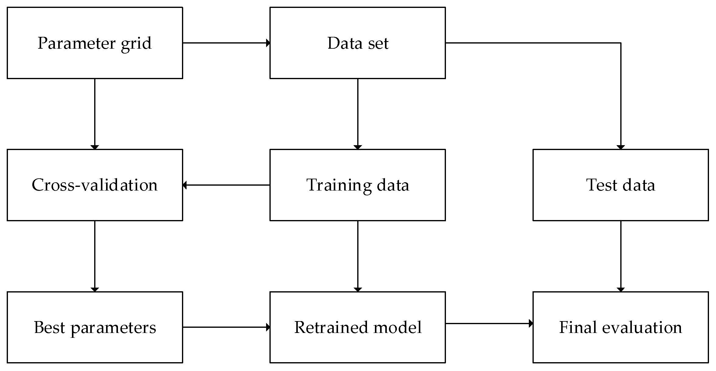
4.1. Random Forest

The dichotomy of CART simplifies the size of the decision tree and improves the efficiency of generation, and is therefore used as a base learner in ensemble algorithms. The default criterion for the CART classification tree corresponding is the Gini coefficient, and the criterion for the selection of the Gini coefficient is that each child node achieves the highest purity, i.e., all observations falling in the child nodes belong to the same classification, at which point the Gini coefficient is minimized, the purity is maximized, and the uncertainty is minimized. The calculation of the metrics is as follows:

$$Gini(D)={\displaystyle \sum _{k=1}^k{p}_k(1-p_k)}=1-{\displaystyle \sum _{k=1}^k{p}_k^2}$$

(1)

$$Gin{i}_{index}(D,a)=\frac{\left|D^1\right|}{D}Gini(D^1)+\frac{\left|D^2\right|}{D}Gini(D^2)$$

(2)

where $D$ is the training dataset sample, $p_k$ is the probability of the sample point belonging to class $K$, $a$ is the set of all possible values for feature $A$, and $D_1$ and $D_2$ are separated from $D$ according $a$.

A Random Forest is an ensemble learning method that builds multiple decision trees and combines their predictions to make more accurate and robust predictions. The construction of a Random Forest consists mainly of the following:

(1)

Construct sample subset. Randomly select N samples from the original training sample set C to generate a new training set, and repeat this process K times to generate K sample sets.

(2)

Construct the genus subspace. For each subsample set, m features are randomly selected from all M random feature variables, m < M.

(3)

Build a decision tree. In the process of generating the Random Forest, K decision trees are generated based on the above constructed subsample sets and generic subspaces, each corresponding to each training subset.

(4)

Construct the Random Forest model. The K decision trees generated in step (2) are combined into a Random Forest, and the model is trained with training data.

4.2. Hyperparameter Adjustment

The decision tree is one of the essential factors for the Random Forest model. Too few trees can lead to underfitting, while the depth of the tree is used to prevent overfitting, and this study uses grid search to select these two hyperparameters. The overview of the process of parameter selection and model evaluation with GridSearchCV.as Figure 2 below.

Grid search is a standard hyperparameter optimization method in machine learning. When training a model, it is often necessary to choose specific hyperparameters to tune the model’s performance, such as learning rate, regularization factor, etc. Grid search optimizes the performance of a model by performing an exhaustive search within a predefined range of hyperparameters to find the best combination of hyperparameters. It is simple, quick, and effective. The maximum tree depth is 4, and the maximum tree is determined as 35.

4.3. Shapley Value and SHAP

The full name of SHAP is SHapley Additive exPlanation, and SHAP is an additive explanatory model inspired by the Shapley value, which originated from cooperative game theory. The SHAP model can show the influencing factors that impact on the final prediction, which improves the machine learning model’s interpretability and also allows for feature importance calculations [42]. For integrated tree models, the model output is a probability value when performing a classification task. Thus, SHAP attributes the output value to the Shapely value of each feature to measure the effect of the feature on the final output value. Notably, SHAP not only displays the degree of influence of each feature variable on the results of each sample, but it also shows the positive or negative nature of the feature contribution.

The weighted average of the marginal contributions of a feature over a subset of all feature combinations is known as the Shapley value; the formula for the Shapley value is:

$${\mathsf{\Phi }}_i={\displaystyle \sum _{S\subseteq (x_1,\cdot \cdot \cdot \cdot \cdot \cdot ,x_M)\backslash x_i}\frac{\left|S\right|!\left(M-\left|S\right|-1\right)!}{M!}}[val(S\cup x_i-val(S)]$$

(3)

where $x_i$ is the $i$-th feature of sample $x$, ${\varphi }_i$ is the contribution of the feature, $S$ is the subset of feature, $M$ is the total number of features. The value function in a machine learning scenario is the model under study and its predicted values, and $S\subseteq (x_1,\cdot \cdot \cdot \cdot \cdot \cdot ,x_M)\backslash x_i$ denotes the set excluding the $x_i$.

When the Shapley value formula with prediction as the value is used to explain the results of the model by adding or subtracting from the predicted value mean to the predicted value, it becomes SHAP (SHapley Additive exPlanation):

$$g\left(z^{(i)}\right)={\varphi }_0^{(i)}+{\displaystyle \sum _{j=1}^M{\varphi }_j^{(i)}{z}_j^{(i)}}$$

(4)

where the symbol $g$ represents the explanatory model; $z$ is the indicator vector of the sample, 1 for the value of the original sample instance of interest, or 0 if replaced by the value of the randomly selected sample; ${\varphi }_0$ is the mean of the predicted values; ${\varphi }_j$ is Shapley value; and ${}^{(i)}$ denotes a particular article/the $i$-th sample.

5. Result and Discussion

5.1. Analysis and Discussion of Results

SHAP is able to explain the predictions by calculating the contribution of each variable to the prediction, and the results are displayed in Figure 3. The x-axis represents the mean absolute value of the overall sample SHAP value, and the y-axis represents the explanatory variables. In this study, we use Python 3.9 software to build and interpret the model through the ‘Random Forest‘ package and ‘SHAP‘ package. The training set and test set are obtained by dividing them in the ratio of 70% and 30%; then, 10% from the training set is taken as the validation set. The finding ranges of n_estimators and max_depth are determined via grid search and cross-validation, and the total number of decision trees in the model and the two parameters of max_depth are optimally tuned. For the RF model on the vehicle-to-vehicle accident, when max_depth = 4 and n_estimators = 35, the highest accuracy rate of 0.7653 is obtained for the training set. Max_feature used auto, and all features can be downscaled, i.e., some features with too low importance can be discarded. The interference of multiple covariance between features in the sample can be removed by choosing sqrt, which stands for choosing root n features for tree building each time. Thus, the interference of multiple covariance between samples is reduced.

As shown in Figure 3, road type and vehicle type significantly impact the severity of accidents, followed by urban/rural, season, speed limit, catering and commercial POIs density, life services POIs density, accident reason, driving experience, and road network density. To determine the direction of feature importance, local interpretation is performed.

Figure 4 summarizes the SHAP values for each feature, with the x-axis representing the SHAP value. A positive SHAP value indicates that the influencing factor positively affects the dependent variable. In contrast, a negative SHAP value suggests that the influencing factor hurts the dependent variable. Each row represents an independent variable that affects the severity of accidents, and each dot represents a sample. Feature values increase gradually from low (blue) to high (red), indicating that the more positive the feature value of the independent variable, the greater its corresponding SHAP value and the more severe the accident.

In summary, the severity of the accident is higher under the following conditions: the road type is a higher-level road; the driver at-fault is driving a motorcar or minivan; the speed limit is high; the cause of the accident is failure to follow signal instructions; the driver is an elderly person or teenager; the location of the accident is in a rural area; the season is winter; the density of the Commercial-POI and network is low; and the density of the Service-POI is high.

An analysis of the impact of each feature on the model output can be made based on this figure:

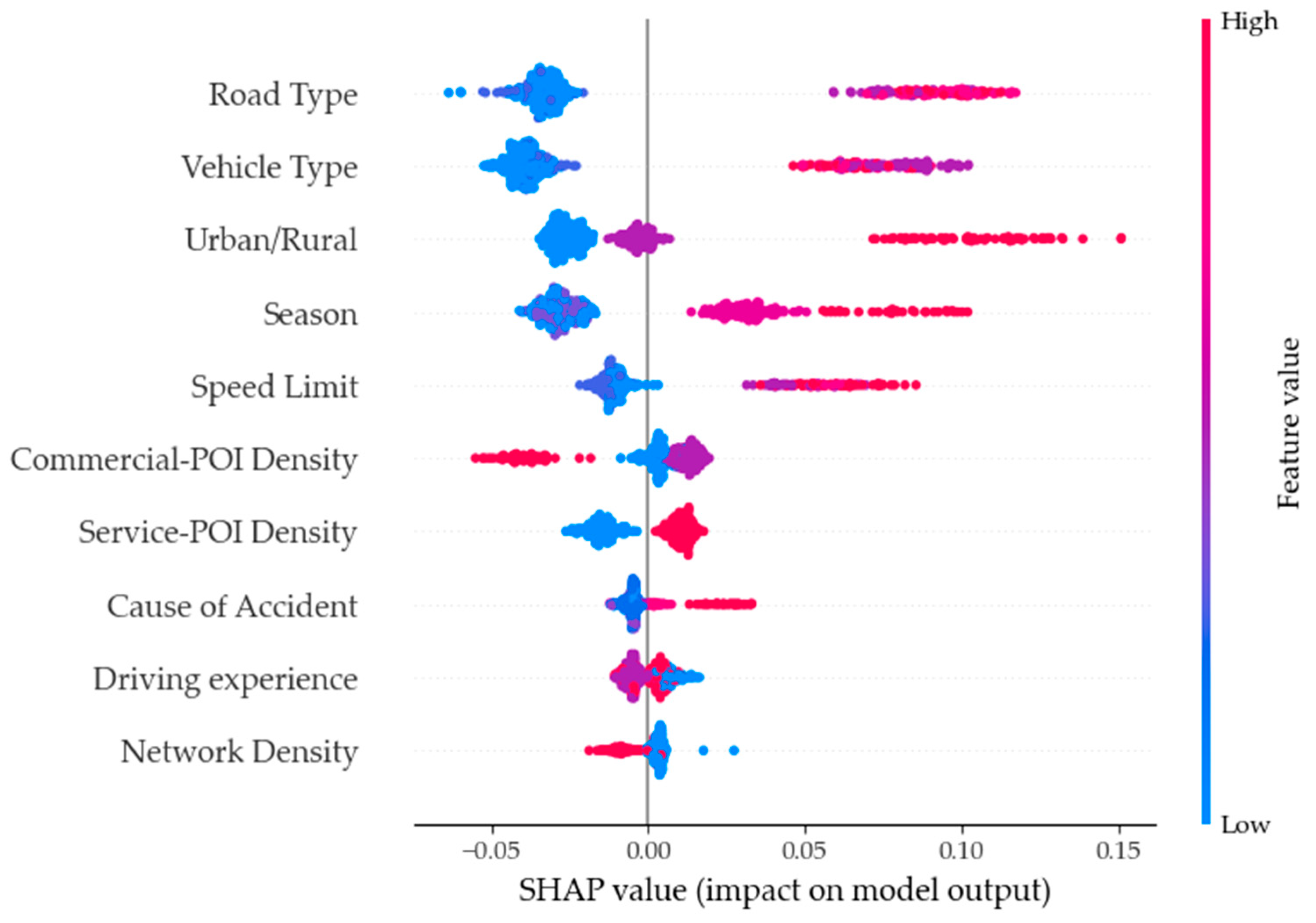
(1)

For road type, as its feature value increases, it positively affects the severity of high-level accidents, such as accidents on urban expressways, which are usually more severe. As its feature value decreases, it harms the severity of high-level accidents, such as accidents on trunk roads or lower-level roads, which are usually less severe. This result was consistent with previous studies’ results [43]. This is consistent with previous studies, and contrary to previous perceptions, low-grade roads may instead have a more negative impact on fatal accidents due to the mandatory restrictions of overly narrow roads or one-way streets, and it is not difficult to find that high-grade roads tend to have higher speed limits in China, so high-speed limits are one of the reasons for the positive impact on fatal accidents.

(2)

Regarding vehicle type, a decrease in its feature value is associated with a negative impact on fatal accidents. Specifically, if the driver at fault is driving a non-motorized vehicle, the effects of vehicle type on fatal accidents are relatively small. However, when the feature value of vehicle type is at an intermediate level, it has a more significant positive effect on fatal accidents than when its feature value is high. In other words, if the driver at fault is driving a minivan or motorcar, the impact of vehicle type on fatal accidents is more considerable than if the driver at fault is driving a non-motorized vehicle. The dataset’s sample size of drivers driving minivans and small trucks is lower; a common phenomenon in general developed cities in China today, where passenger car travel is prevalent. However, the construction of road infrastructure still leaves much to be desired and can create traffic congestion in most areas, leading to higher accident rates and high severity of accidents.

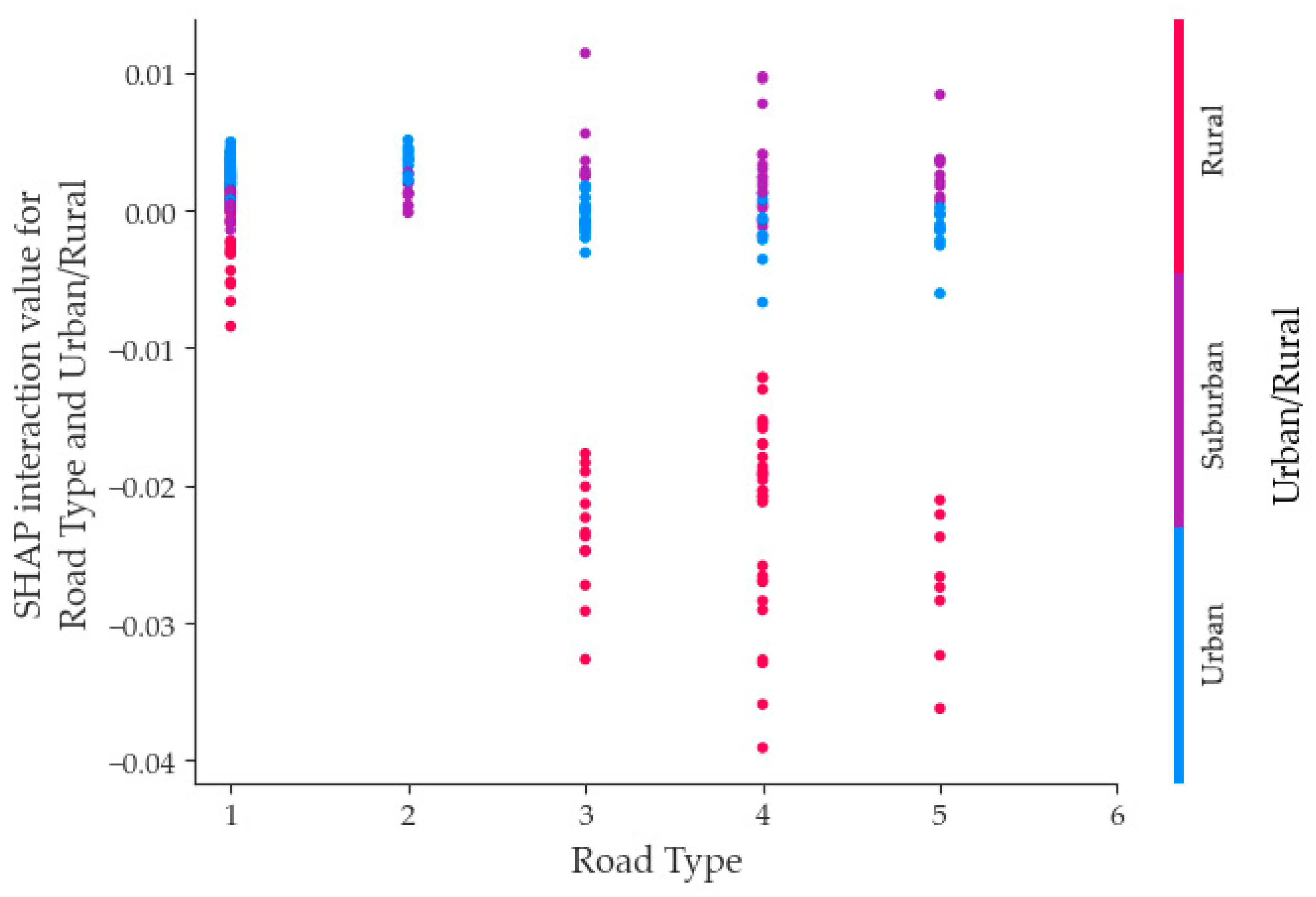
(3)

For urban/rural areas, the two colors of its feature values correspond to urban (blue) and rural (red). The areas where the SHAP values are less than zero are mainly blue points, indicating a negative effect on the severity of accidents, i.e., the possibility of minor accidents is greater when accidents occur in urban districts. The areas where the SHAP values are greater than zero are mainly red points, indicating a positive effect on the severity of accidents, i.e., accidents in rural districts are usually more severe [43]. The positive effect of suburban areas on fatal accidents is much more significant than that of urban areas, which is similar to the principle mentioned above, precisely because of the developed road network in cities and towns. Meanwhile, suburban areas are primarily national or provincial roads, so drivers are less alert, thus having a positive effect on fatal accidents, which is corroborated by the result that lower road network density has a more positive impact.

(4)

For speed limit, as its feature value increases, it positively affects the severity of accidents, i.e., the higher the speed limit, the more severe the accident. Similar findings have been generated in previous studies [44]. As its feature value decreases, it has a negative effect on the severity of accidents, i.e., the lower the speed limit, the less severe the accident.

(5)

For the age of the driver, as its feature value increases or decreases, it has a positive effect on the severity of accidents, i.e., the higher or lower the age range of the driver, the more severe the accident. This is related to driver behavior psychology, as research shows that middle-aged drivers have safer driving styles, while young people may have more impulsive or less experienced driving skills. In traffic behavior psychology studies, drivers who are too young lack driving experience and are prone to rashness and recklessness, while drivers who are too old have a low reaction time and lose their ability to handle emergencies or lag in their reactions [36], so these people have higher accident severity than middle-aged people.

(6)

For season, the severity of accidents corresponds to multiple feature values, but the positive SHAP values mainly consist of red dots, indicating that accidents occurring in winter tend to be more severe. This is due to the distinct feature of long winters in Shenyang, China, where most days between November and March have low temperatures and snowy weather, resulting in worse road conditions and more severe accidents [17]. This result also indirectly demonstrates that weather may have an impact on the severity of accidents. Shenyang is one of the cities in northeastern China, and the most crucial feature of this region is the long winter season, up to six months, half of the year in a low-temperature environment, where road conditions are complicated by low temperatures or snowfall, requiring a high level of driving operation and vehicle performance. Therefore, the long winter season has had a positive impact on fatal accidents.

(7)

For Service-POI density, as its feature value increases, it has a positive effect on the severity of accidents, indicating that when the density of the POI is high, the severity of accidents tends to be higher. This result was consistent with previous studies’ results [38]. As its feature value decreases, it has a negative effect on the severity of accidents, indicating that when the density of the Service-POI density is low, the severity of accidents tends to be lower.

(8)

For the cause of the accident, as its feature value increases, it has a positive effect on the severity of accidents, indicating that when the cause of accidents is failure to follow signal instructions, the severity of accidents tends to be higher [40]. As its feature value decreases, it has a negative effect on the severity of accidents, indicating that when the cause of accidents is the improper operation of the driver, the severity of accidents tends to be lower. In Shenyang, motor vehicles’ disobedience of signals can be very costly, while non-motorized vehicles and pedestrians do not have better enforcement, especially with the development of the take-out industry, which is more prominent. Often disobeying signals is more likely to produce fatal accidents and is also a more oriented result. After all, extreme penalties for drivers who violate signal rules have been incorporated into Chinese traffic laws.

(9)

For network density, as its feature value decreases, it positively affects the severity of accidents, indicating that when the road network density is low, the severity of accidents tends to be higher. As its feature value increases, it has a negative effect on the severity of accidents, indicating that when the road network density is high, the severity of accidents tends to be lower. Meanwhile, in a study by Zafri et al. [45], they found that higher road network density has a positive effect on fatalities in pedestrian accidents.

(10)

For Commercial-POI density, as its feature value decreases, it positively affects the severity of accidents, indicating that when the density of the Commercial-POI is low, the severity of accidents tends to be higher [46]. As its feature value increases, it has a negative effect on the severity of accidents, indicating that when the density of the Commercial-POI is high, the severity of accidents tends to be lower.

In a previous study, we observed the trend of the top ten single-factor effects on accidents, and the results showed that low- and medium-density Commercial-POIs caused more serious accidents. At the same time, high-density Service-POIs presented a positive impact on accidents. We have not been able to clarify the specific principle of the effect POI density, which was glimpsed in the two-factor interaction in order to explore the possible reasons for its contribution to fatal accidents [37]. A two-factor interaction analysis is performed on the top ten most important influencing factors, and significant characteristics arising between the different factors are found.

Figure 5 shows that the importance of the characteristic variables changes when the road type interacts with the season. High-rated roads are more likely to produce non-fatal crashes in winter, while high-rated roads are more likely to have fatal crashes in spring and summer. The potential impact of crashes is considered in subsequent studies. Main roads and other types of roads, which may be paved with dirt or concrete, are more likely to be icy in the winter due to cold and wet conditions, and poorer road conditions can create other situations that can lead to hazards or the high-risk nature of the environment.

As mentioned, traffic environments in dense urban areas are safer than low-traffic environments in suburban areas because there are far fewer miles traveled per capita, and the lower travel speeds make fatal accidents less likely. However, a more nuanced conclusion emerges from the results of the interaction. Figure 6 shows that a suburban area has a higher impact on fatal accidents, but high-level roads in rural areas have a higher promotional effect on non-fatal accidents. Therefore, we think that we should further regulate the penalties and strengthen the density of electronic enforcement in rural areas; strengthen the road infrastructure in rural areas, such as by improving crosswalks or underpasses; and enhance education to strictly prohibit pedestrians from crossing the road.

As shown in Figure 7 and Figure 8, the results are the opposite in the traffic pattern interaction of the commercial area and the traffic pattern interaction of the living service area. In our definition, locations such as dining, food, shopping, and leisure are included under Commercial-POIs, while Service-POIs include express pickup centers, transit freight centers, hair salons, laundries, and supermarkets, etc.

Non-motorized vehicles and motorcycles are more likely to cause fatal accidents in areas with high Commercial-POI densities greater than 500 pcs/km² and minivans, large passenger trucks, and others within the low-density Commercial-POI area of 0–50 pcs/km². We speculate this is mainly since, in areas with restaurants, these areas are also closely associated with take-out platforms, which require employees to complete orders within a limited time frame, resulting in frequent illegal driving, thus generating a high incidence of accidents involving non-motorized vehicles and motorcycles, which has increased the number of fatal accidents in which the driver is at fault. In contrast, the travel rate of motor vehicles and other medium and large vehicles increases in areas with lower Commercial-POI density. The density of Service-POIs is not as high as Commercial-POIs due to the spatial distribution of cities in developing countries, the spatial distribution pattern, and the different needs of residents. The likelihood of fatal accidents increases under the influence of non-motorized, motorcycle, and other types of vehicle negligence and low-density Service-POI. Under low-density Service-POI conditions, the impact of non-fatal crashes is higher for cars and minivans, with ambiguous results for large trucks.

In the results of the interaction between Commercial-POI density and Service-POI density and vehicle type, it is easy to find that the supervision of non-motorized vehicles and motorcycles should be strengthened to reduce the accident rate. In the study by Wang et al. [47], the factors influencing the occurrence of accidents on e-bikes in China were pointed out, and in the study by Outay et al. [48] it was also pointed out that motorcycle accidents are more serious during peak hours, which may be related to severe braking or acceleration events. In a study by Zhu et al. [49] it was found that people with the same socio-economic background were more likely to be involved in accidents between bicycles and other vehicles.

As population density increases, activity trajectory is broader, and there is an increase in peak hour travel, which all need to take into consideration the built environment as the premise of the analysis of the accident impact factors. Similar conclusions were found in the above article, which also confirms that no matter what kind of results or entry point explored, they are inextricably linked with the environment. This paper aimed to explore the points of interest and road network density, which is a cutting-edge research trend. This is very important for the study of road traffic safety, which can optimize the regional configuration from the perspective of future urban planning and reduce the possibility of serious accidents from the root.

5.2. Selected Sources of Research Methodology

The methods chosen in this paper refer to previous studies, based on the type of data source; the effectiveness of the methods and whether they are cutting-edge or not were compared. By referring to the articles of Ding [24], Ewing [25], Ahmad [26], Wen [37], etc., we have found that the machine learning approach has a great advantage over the traditional regression model in that it can train high-latitude data and does not have to perform feature selection. Even if a large portion of the features are missing, the Random Forest algorithm can still maintain its accuracy, the prediction results are not affected by multicollinearity, and so on. In particular, Random Forest is able to solve both types of problems, i.e., classification and regression, and performs well in both. However, Random Forest is usually used to solve classification problems, and the article [40] refers to classification studies in the industry. The final dependent variable chosen is accident severity, which is categorized into fatal and non-fatal. At the same time, the article considered the influence of the built environment as part of the research based on the spatial distribution characteristics of the study. After considering the consistency with the overall content of the article and referring to other authors of related research, there is too little of this type of data and machine learning models in this paper to match the degree of the final discarded analysis of spatial characteristics. This will also be taken into consideration as a direction of our future research, such as the study of accident frequency based on a spatio-temporal perspective.

6. Conclusions

This study analyzes mixed motorized and non-motorized traffic accident data, focusing on the responsible party’s perspective in Shenyang, Liaoning Province, China, from 2018 to 2020. The primary objective is to explore the factors that have a greater impact on fatal/non-fatal accidents and their negative/positive trends, as well as to explore if, under the condition that one type of factor is known to have a strong impact on accidents with fatalities, whether another type of factor, on this basis, would interact with another to have a different mechanism of action on fatal accidents. The key research findings are outlined as follows:

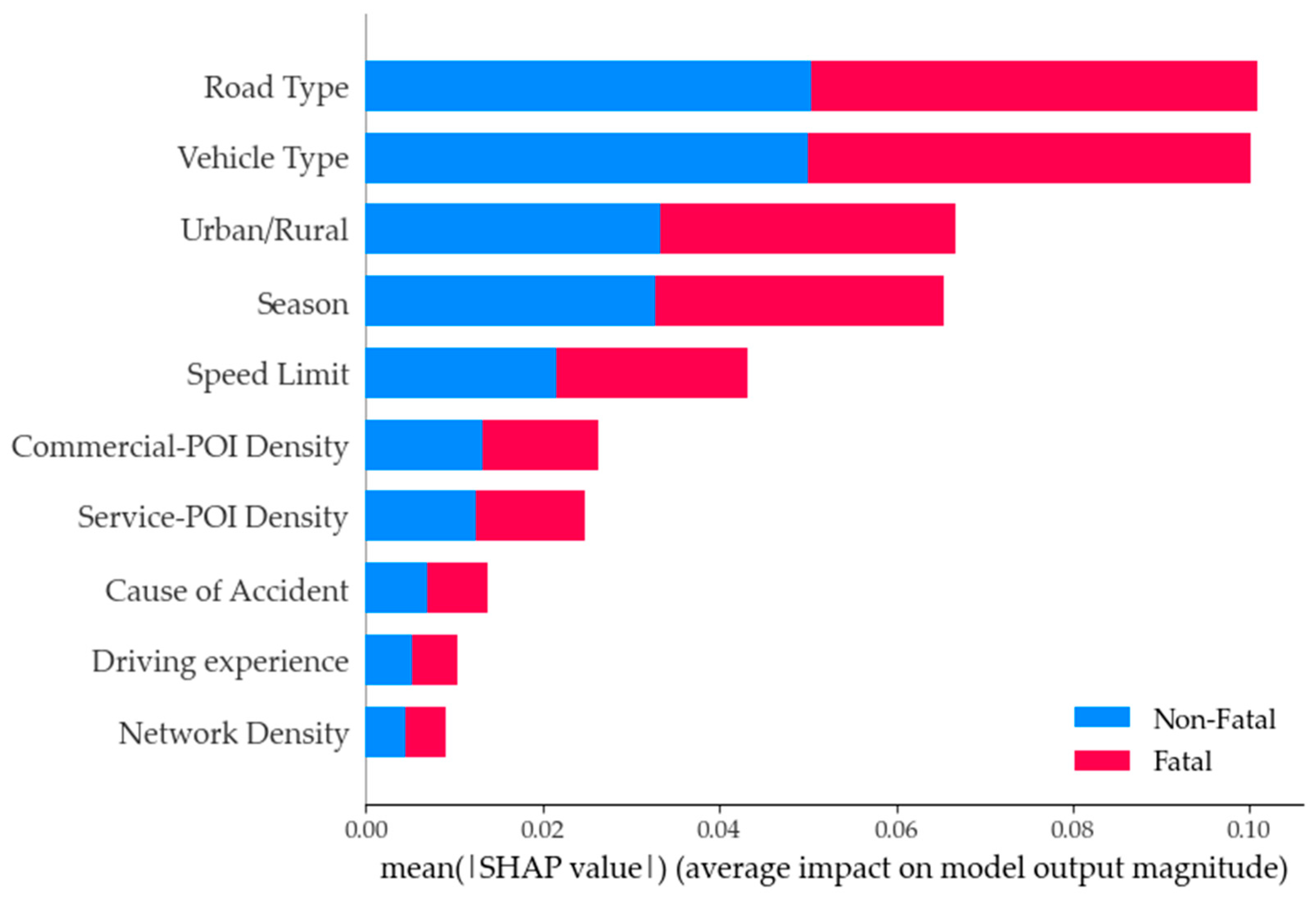
• The Shenyang data underwent descriptive statistical analysis and variable classification processing. To assess the importance and influence of 23 accident-related factors, the Random Forest and SHAP methods were employed. The results demonstrate that the most significant feature impacting accident severity is road type, followed by vehicle type, urban/rural, season, speed limit, Commercial-POI, Service-POI, cause of accident, age of driver, and network. Fatal accidents are more likely to occur on high-grade roads, particularly when involving small passenger and cargo vehicles in rural areas and during winter. Additional contributing factors included high speed limits, failure to adhere to signal instructions, varying driver experience levels, and the moderately low density of Commercial-POIs and road networks.
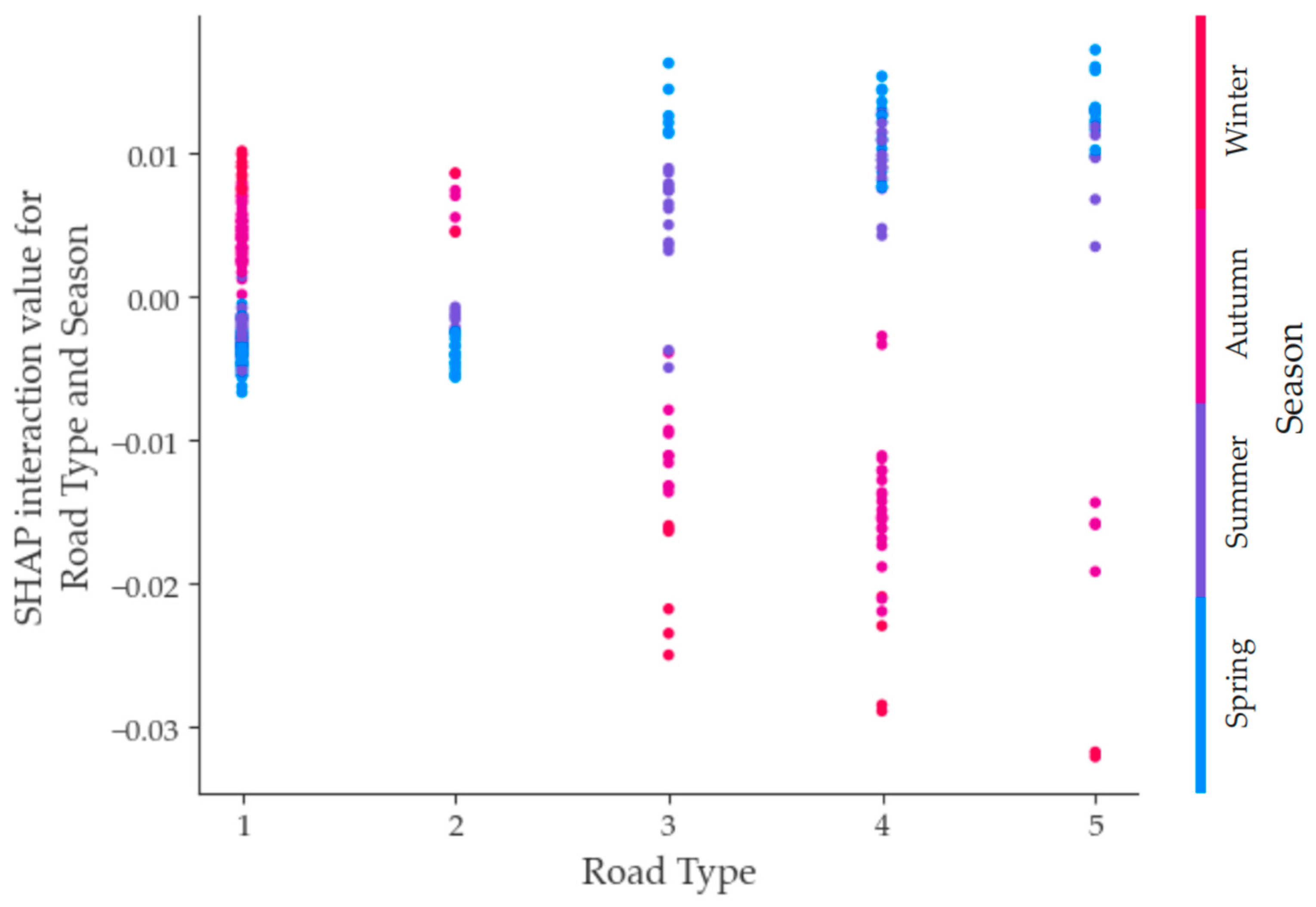
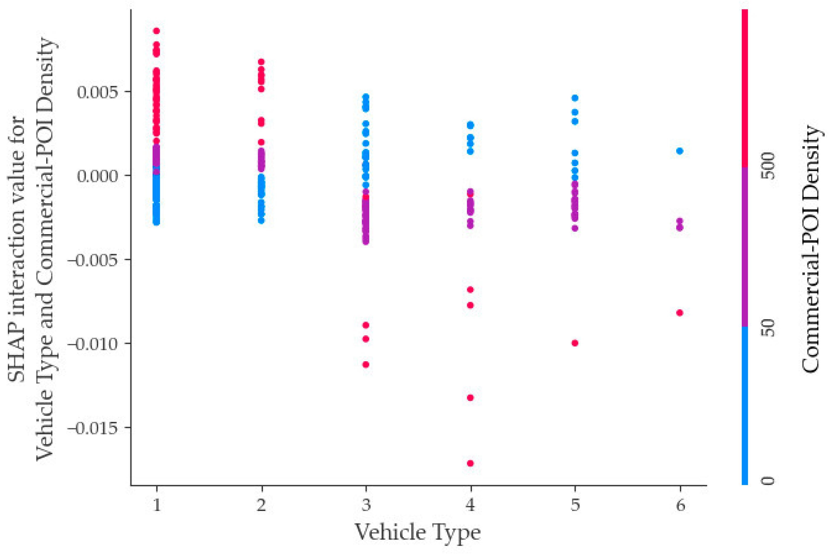
• Focusing on the top 10 selected variables, this study delved into the mechanism of influence regarding fatal accidents within the context of two-factor interactions. The findings indicate that the interaction between road type and season, vehicle type and Commercial-POI, as well as road type and urban/rural displayed noteworthy characteristics concerning fatal accidents. Consequently, this investigation contributes theoretical support to traffic management.

The innovation of this paper is to draw on vehicle-to-vehicle accident data from the extreme cold region of mainland China, which not only includes a single source of traffic police report data present in previous studies, but also self-acquired data based on the built environment. The results reveal that in addition to human factors, environmental influences also play a key role in fatal accidents. Where factors were significant in the single factor results, the authors went on to explore two-factor effects, demonstrating interesting results. In this article, although SHAP compensates for the usual problem of poor model interpretability, the two-factor interaction mechanism of SHAP can only be explored by artificially screening the interaction factors. The two-factor and even multi-factor interaction mechanisms are explored. In the future, we will include more factors in considering the built environment. Furthermore, we will consider the exploration multi-factor interaction mechanisms using association rule algorithms such as Apriori.

References

- World Health Organization. Global Status Report on Road Safety 2020; World Health Organization: Geneva, Switzerland, 2020. [Google Scholar]
- Liu, P.; Fan, W. Exploring injury severity in head-on crashes using latent class clustering analysis and mixed logit model: A case study of North Carolina. Accid. Anal. Prev. 2020, 135, 105388. [Google Scholar] [CrossRef]
- Liu, J.; Hainen, A.; Li, X.; Nie, Q.; Nambisan, S. Pedestrian injury severity in motor vehicle crashes: An integrated spatio-temporal modeling approach. Accid. Anal. Prev. 2019, 132, 105272. [Google Scholar] [CrossRef]
- Li, Y.; Song, L.; Fan, W.D. Day-of-the-week variations and temporal instability of factors influencing pedestrian injury severity in pedestrian-vehicle crashes: A random parameters logit approach with heterogeneity in means and variances. Anal. Methods Accid. Res. 2021, 29, 100152. [Google Scholar] [CrossRef]
- Song, D.; Yang, X.; Zu, X.; Si, B. Examination of Driver Injury Severity in Urban Crashes: A Random Parameters Logit Model with Heterogeneity in Means Approach. J. Transp. Syst. Eng. Inf. Technol. 2021, 21, 214–220. [Google Scholar]
- Shen, X.; Shen, J.; Zheng, C.; Yu, M. Severity Analysis of Slow Traffic Accidents in North Carolina Based on Multinomial Logit Model. Traffic Transp. 2021, 37, 24–28. [Google Scholar]
- Clifton, K.J.; Burnier, C.V.; Akar, G. Severity of injury resulting from pedestrian–vehicle crashes: What can we learn from examining the built environment? Transp. Res. Part D Transp. Environ. 2009, 14, 425–436. [Google Scholar] [CrossRef]
- Hosseinzadeh, A.; Moeinaddini, A.; Ghasemzadeh, A. Investigating factors affecting severity of large truck-involved crashes: Comparison of the SVM and random parameter logit model. J. Saf. Res. 2021, 77, 151–160. [Google Scholar] [CrossRef]
- Ahmed, S.; Hossain, M.A.; Ray, S.K.; Bhuiyan, M.M.I.; Sabuj, S.R. A study on road accident prediction and contributing factors using explainable machine learning models: Analysis and performance. Transp. Res. Interdiscip. Perspect. 2023, 19, 100814. [Google Scholar] [CrossRef]
- Parsa, A.B.; Movahedi, A.; Taghipour, H.; Derrible, S.; Mohammadian, A.K. Toward safer highways, application of XGBoost and SHAP for real-time accident detection and feature analysis. Accid. Anal. Prev. 2020, 136, 105405. [Google Scholar] [CrossRef]
- Yang, Y.; Yuan, Z.; Meng, R. Exploring Traffic Crash Occurrence Mechanism toward Cross-Area Freeways via an Improved Data Mining Approach. J. Transp. Eng. Part A Syst. 2022, 148, 04022052. [Google Scholar] [CrossRef]
- Ahmad, N.; Ahmad, A.; Wali, B.; Saeed, T.U. Exploring factors associated with crash severity on motorways in Pakistan. Proc. Inst. Civ. Eng.-Transp. 2022, 175, 189–198. [Google Scholar] [CrossRef]
- Se, C.; Champahom, T.; Jomnonkwao, S.; Karoonsoontawong, A.; Ratanavaraha, V. Temporal stability of factors influencing driver-injury severities in single-vehicle crashes: A correlated random parameters with heterogeneity in means and variances approach. Anal. Methods Accid. Res. 2021, 32, 100179. [Google Scholar] [CrossRef]
- Li, Y.; Zhang, X.; Wang, W.; Ju, X. Factors Affecting Electric Bicycle Rider Injury in Accident Based on Random Forest Model. J. Transp. Syst. Eng. Inf. Technol. 2021, 01, 196–200. [Google Scholar]
- Zhu, X.; Srinivasan, S. A comprehensive analysis of factors influencing the injury severity of large-truck crashes. Accid. Anal. Prev. 2011, 43, 49–57. [Google Scholar] [CrossRef]
- Yang, Y.; Wang, K.; Yuan, Z.; Liu, D. Predicting Freeway Traffic Crash Severity Using XGBoost-Bayesian Network Model with Consideration of Features Interaction. J. Adv. Transp. 2022, 2022, 4257865. [Google Scholar] [CrossRef]
- Adanu, E.K.; Agyemang, W.; Islam, R.; Jones, S. A comprehensive analysis of factors that influence interstate highway crash severity in Alabama. J. Transp. Saf. Secur. 2022, 14, 1552–1576. [Google Scholar] [CrossRef]
- Jiao, P.; Li, R.; Wang, J.; Ge, H.; Chen, Y. Causes Analysis on Severity of Elderly Pedestrian Crashes Considering Latent Classes. J. Transp. Syst. Eng. Inf. Technol. 2022, 05, 328–336. [Google Scholar]
- Kullgren, A.; Stigson, H.; Ydenius, A.; Axelsson, A.; Engström, E.; Rizzi, M. The potential of vehicle and road infrastructure interventions in fatal bicyclist accidents on Swedish roads—What can in-depth studies tell us? Traffic Inj. Prev. 2019, 20, S7–S12. [Google Scholar] [CrossRef]
- Tay, R.; Rifaat, S.M. Factors contributing to the severity of intersection crashes. J. Adv. Transp. 2007, 41, 245–265. [Google Scholar] [CrossRef]
- Jiang, C.; He, J.; Zhu, S.; Zhang, W.; Li, G.; Xu, W. Injury-Based Surrogate Resilience Measure: Assessing the Post-Crash Traffic Resilience of the Urban Roadway Tunnels. Sustainability 2023, 15, 6615. [Google Scholar] [CrossRef]
- Yang, Y.; Tian, N.; Wang, Y.; Yuan, Z. A Parallel FP-Growth Mining Algorithm with Load Balancing Constraints for Traffic Crash Data. Int. J. Comput. Commun. Control 2022, 17, 4806. [Google Scholar] [CrossRef]
- Zeng, Q.; Wang, X.; Zhang, X.; Wen, H. Seasonal Analysis of Contributing Factors to Freeway Crash Frequency Using a Spatio-temporal lnteraction Model. China J. Highw. Transp. 2020, 33, 255–263. [Google Scholar]
- Ding, C.; Chen, P.; Jiao, J. Non-linear effects of the built environment on automobile-involved pedestrian crash frequency: A machine learning approach. Accid. Anal. Prev. 2018, 112, 116–126. [Google Scholar] [CrossRef]
- Ewing, R.; Dumbaugh, E. The Built Environment and Traffic Safety: A Review of Empirical Evidence. J. Plan. Lit. 2009, 23, 347–367. [Google Scholar] [CrossRef]
- Ahmad, N.; Wali, B.; Khattak, A.J.; Dumbaugh, E. Built environment, driving errors and violations, and crashes in naturalistic driving environment. Accid. Anal. Prev. 2021, 157, 106158. [Google Scholar] [CrossRef]
- Muhammad, U.; Irfan, A.R.; Rida, H.L. The impact of urban design and the built environment on road traffic crashes: A case study of Rawalpindi, Pakistan. Case Stud. Transp. Policy 2022, 10, 417–426. [Google Scholar]
- Lee, S.; Yoon, J.; Woo, A. Does elderly safety matter? Associations between built environments and pedestrian crashes in Seoul, Korea. Accid. Anal. Prev. 2020, 144, 105621. [Google Scholar] [CrossRef] [PubMed]
- Merlin, L.A.; Guerra, E.; Dumbaugh, E. Crash risk, crash exposure, and the built environment: A conceptual review. Accid. Anal. Prev. 2019, 134, 105244. [Google Scholar] [CrossRef]
- Nam, D.; Mannering, F. An exploratory hazard-based analysis of highway incident duration. Transp. Res. Part A Policy Pract. 2000, 34, 85–102. [Google Scholar] [CrossRef]
- Huang, H.; Chin, H.C.; Haque, M.M. Severity of driver injury and vehicle damage in traffic crashes at intersections: A Bayesian hierarchical analysis. Accid. Anal. Prev. 2008, 40, 45–54. [Google Scholar] [CrossRef]
- Haleem, K.; Gan, A. Contributing factors of crash injury severity at public highway-railroad grade crossings in the U.S. J. Saf. Res. 2015, 53, 23–29. [Google Scholar] [CrossRef] [PubMed]
- Wang, J.; Lu, H.; Sun, Z.; Wang, T. Identification method of factors influencing the severity of vehicle collision crashes based on MNL model. Highw. Traffic Sci. Technol. 2021, 38, 107–113. [Google Scholar]
- Xu, R.; Luo, F. Risk prediction and early warning for air traffic controllers’ unsafe acts using association rule mining and random forest. Saf. Sci. 2021, 135, 105125. [Google Scholar] [CrossRef]
- Yang, Y.; He, K.; Wang, Y.P.; Yuan, Z.; Yin, Y.H.; Guo, M. Identification of dynamic traffic crash risk for cross-area freeways based on statistical and machine learning methods. Phys. A Stat. Mech. Its Appl. 2022, 595, 127083. [Google Scholar] [CrossRef]
- Das, A.; Abdel-Aty, M.; Pande, A. Using conditional inference forests to identify the factors affecting crash severity on arterial corridors. J. Saf. Res. 2009, 40, 317–327. [Google Scholar] [CrossRef]
- Wen, X.; Xie, Y.; Wu, L.; Jiang, L. Quantifying and comparing the effects of key risk factors on various types of roadway segment crashes with LightGBM and SHAP. Accid. Anal. Prev. 2021, 159, 106261. [Google Scholar] [CrossRef]
- Chang, I.; Park, H.; Hong, E.; Lee, J.; Kwon, N. Predicting effects of built environment on fatal pedestrian accidents at location-specific level: Application of XGBoost and SHAP. Accid. Anal. Prev. 2022, 166, 106545. [Google Scholar] [CrossRef] [PubMed]
- Yang, C.; Chen, M.; Yuan, Q. The application of XGBoost and SHAP to examining the factors in freight truck-related crashes: An exploratory analysis. Accid. Anal. Prev. 2021, 158, 106153. [Google Scholar] [CrossRef]
- Wang, Z.; Jiao, P.; Wang, J.; Huang, Q.; Li, R.; Lu, H. The level of delay caused by crashes (LDC) in metropolitan and non-metropolitan areas: A comparative analysis of improved Random Forests and LightGBM. Int. J. Crashworthiness 2022. [Google Scholar] [CrossRef]
- Choi, D.; Ewing, R. Effect of street network design on traffic congestion and traffic safety. J. Transp. Geogr. 2021, 96, 103200. [Google Scholar] [CrossRef]
- Lundberg, S.M.; Lee, S.I. A unified approach to interpreting model predictions. Adv. Neural Inf. Process. Syst. 2017, 30, 4765–4774. [Google Scholar]
- Goswamy, A.; Abdel-Aty, M.; Islam, Z. Factors affecting injury severity at pedestrian crossing locations with Rectangular RAPID Flashing Beacons (RRFB) using XGBoost and random parameters discrete outcome models. Accid. Anal. Prev. 2023, 181, 106937. [Google Scholar] [CrossRef]
- Dash, I.; Abkowitz, M.; Philip, C. Factors impacting bike crash severity in urban areas. J. Saf. Res. 2022, 83, 128–138. [Google Scholar] [CrossRef] [PubMed]
- Zafri, N.M.; Khan, A. A spatial regression modeling framework for examining relationships between the built environment and pedestrian crash occurrences at macroscopic level: A study in a developing country context. Geogr. Sustain. 2022, 3, 312–324. [Google Scholar] [CrossRef]
- Cai, Q.; Abdel-Aty, M.; Zheng, O.; Wu, Y. Applying machine learning and google street view to explore effects of drivers’ visual environment on traffic safety. Transp. Res. Part C Emerg. Technol. 2022, 135, 103541. [Google Scholar] [CrossRef]
- Wang, X.; Chen, J.; Quddus, M.; Zhou, W.; Shen, M. Influence of familiarity with traffic regulations on delivery riders’ e-bike crashes and helmet use: Two mediator ordered logit models. Accid. Anal. Prev. 2021, 159, 106277. [Google Scholar] [CrossRef] [PubMed]
- Outay, F.; Adnan, M.; Gazder, U.; Baqueri, S.F.A.; Awan, H.H. Random forest models for motorcycle accident prediction using naturalistic driving based big data. Int. J. Inj. Control Saf. Promot. 2023, 30, 282–293. [Google Scholar] [CrossRef] [PubMed]
- Zhu, C.; Brown, C.T.; Dadashova, B.; Ye, X.; Sohrabi, S.; Potts, I. Investigation on the driver-victim pairs in pedestrian and bicyclist crashes by latent class clustering and random forest algorithm. Accid. Anal. A Prev. 2023, 182, 106964. [Google Scholar] [CrossRef]