Article

Land Use Regression Models for Particle Number Concentration and Black Carbon in Lanzhou, Northwest of China

1
College of Atmospheric Sciences, Lanzhou University, Lanzhou 730000, China
2
School of Public Health, Gansu University of Chinese Medicine, Lanzhou 730000, China
*
Author to whom correspondence should be addressed.
Sustainability 2023, 15(17), 12828; https://doi.org/10.3390/su151712828
Submission received: 27 June 2023 / Revised: 11 August 2023 / Accepted: 21 August 2023 / Published: 24 August 2023

Abstract

:
It is necessary to predict the spatial variation in particle number concentration (PNC) and black carbon (BC) because they are considered air pollutants associated with traffic and many diseases. In this study, land use regression (LUR) models for PNC and BC were developed based on a mobile monitoring campaign in January 2020 in Lanzhou, and the performance of models was evaluated with hold-out validation (HV) and leave-one-out cross-validation (LOOCV). The results show that the adjusted R2 of the LUR models for PNC and BC are 0.51 and 0.53, respectively. The R2 of HV and LOOCV are 0.43 and 0.44, respectively, for the PNC model and 0.42 and 0.50, respectively, for the BC model. The performances of the LUR models are of a moderate level. The spatial distribution of the predicted PNC is related to the distance from water bodies. The high PNC is related to industrial pollution. The BC concentration decreases from south to north. High BC concentrations are associated with freight distribution centres and coal-fired power plants. The range of PNC particle sizes in this study is larger than in most studies. As one of few studies in Lanzhou to develop LUR models of air pollutants, it is important to accurately estimate pollutant concentrations to improve air quality and provide health benefits for residents.

1. Introduction

Epidemiological studies have shown that even modest increases in air pollution may lead to substantial negative health consequences at the population level owing to the ubiquity of exposure [1,2], with considerable socio-economic impacts [3]. Consequently, air pollution remains an important global environmental and public health concern [4]. Increasing evidence indicates that traffic-related air pollutants (TRAPs) lead to numerous adverse health effects and that particle number concentration (PNC) and black carbon (BC) are associated with air pollution [5]. Some scholars have reported that PNC may affect the adverse association between particulate matter and respiratory health and increase the risk of cardiovascular mortality. Particularly, the adverse health effects of PNC on stagnant air masses may be greater [6,7]. BC is a useful indicator of the adverse health effects of traffic-related air pollution [8]. Several studies have reported mortality rates comparable to PM10 or even higher for short-term exposure at sites with higher EC concentrations and a stronger association between BC and mortality than PM2.5 [9,10]. For cardiopulmonary mortality, the effects of elemental carbon were approximately seven and eight times greater than those of sulphate and PM2.5, respectively [11]. An increase in the interquartile range for BC (2.7 mg/m3) corresponded to increases in total, cardiovascular, and respiratory mortality of 2.3%, 3.2%, and 0.6%, respectively [12]. Some studies have shown that BC accelerates the formation of atherosclerotic plaques, suggesting long-term effects on cardiovascular health [11,13]. BC is thought to be inextricably linked to pneumoconiosis and is associated with increased respiratory symptoms, a slight decrease in lung function, and the accumulation of dust in the lungs [14,15]. Owing to the high spatial and temporal variability in PNC and BC concentrations, it is important to accurately assess pollutant concentrations when exploring their health effects.
However, a major reason we know less about PNC and BC exposure than PM and ozone exposure is the lack of large-scale monitoring networks. There are few monitoring stations for PNC and BC because they are not routinely monitored by ambient air quality state-controlled automatic monitoring stations, and the monitoring data are limited [16]. Another important reason is that the monitoring instruments for PNC and BC are relatively expensive. The lack of data on PNC and BC poses a significant challenge in assessing their health effects. Studies investigating PNC and BC concentrations are primarily based on fixed-site ambient measurements. Because of traffic (mobile and widely distributed) and solid fuel burning (fixed and sparsely distributed) emissions, fixed-site measurements are insufficient to adequately monitor air quality in large urban areas [17,18,19]. This affects the resolution of air pollution maps/forecast models based on datasets generated by these devices [3]. Only a handful of studies have used mobile platforms for PNC and BC characterisation. Extreme peak values characterise mobile monitoring in particle concentrations that are not visible in fixed-site measurements and can capture the high variability in PNC and BC in complex urban terrain. Mobile measurements with portable and precise measurement devices provide the opportunity to monitor local air quality. Their low cost makes them suitable for large-scale applications and the construction and exploitation of high-resolution maps obtained from many single measurements [1,3,20]. Using highly time-resolved instruments installed in mobile monitoring laboratories proved useful for mapping particles’ spatiotemporal variability over a medium-sized urban area. It can improve the spatial resolution of stationary monitoring stations and discover hotspots [21,22].
Since LUR models were first used to assess within-city variations in air pollution by Briggs et al., they have increasingly been used to predict yearly or seasonal changes in exposure to ambient air pollution for current or recent periods [23,24,25]. Land use regression (LUR) is a technique that uses geographical information systems (GIS) and statistical analyses to quantify multivariate relationships between geographic features (e.g., surrounding land use characteristics, road network, traffic, physical environment, and population) and the monitoring of air pollutant measurements to predict air pollutant concentrations at a given site using the parameter estimates derived from the regression model [26,27]. Most small-scale variations in pollutant concentrations are not identifiable, and extrapolation accuracy is poor using most interpolation techniques based on monitoring network density and spatial distribution of traffic sources; however, LUR models account for small-scale variations in intraurban pollutant concentrations and provide good results for rather low complexity [19,28,29]. Several LUR models have been developed for the PNC and BC. Very few studies have been conducted on LUR modelling for total PNC. Rahman et al. compared the performance of LUR models for PNC developed by two algorithms [30], and Liu et al. collected data from urban and rural PNC along a fixed walking route to build LUR models that complemented the estimated exposure to pollutant concentrations needed for human health risk assessment in a given environment [31,32]. Most scholars have developed LUR models using PNC instead of ultrafine particles (UFPs) concentration to estimate the effects of UFP on human health; however, they measured a much smaller range of particle diameters than in this study [5,33,34,35,36,37,38]. For the LUR models of BC, some studies have used concentrations measured at fixed stations for modellings, such as Boniardi et al., who developed seasonal and annual models for Milan from data from 34 monitoring sites and 1 reference site [39]. Many studies have used mobile monitoring to determine the pollutant concentrations. Some chose mobile monitoring via vehicles [40,41], while others chose other methods [42]. However, owing to the limitation of monitoring data, there are few reports on the LUR modelling of BC in China. Vehicles have been used for mobile monitoring to obtain data in most of these studies [43,44], and there are no previous studies on LUR models using total PNC.
The complex urban structure causes significant spatio-temporal variation in PNC and BC, and the sparse fixed-site monitoring in urban areas can often only represent the air conditions in and around typical functional areas and does not reflect fine spatial distribution of air pollutants within cities well. In order to fully understand the intraurban variability in PNC and BC, contributing to more accurate exposure assessments and reducing misclassification of air pollution health effects, this study measured PNC and BC concentrations in an urban area of Lanzhou, China using a mobile monitoring platform between 8 and 17 January 2020. This study aimed to develop LUR models to produce high-resolution predicted maps of pollutant concentrations. Section 2 presents the data and methods used in this study. In Section 3, the results and performance of the LUR models developed in this study for PNC and BC are presented, and the model is compared with models from other studies. Section 4 summarises the results of this study.

2. Materials and Methods

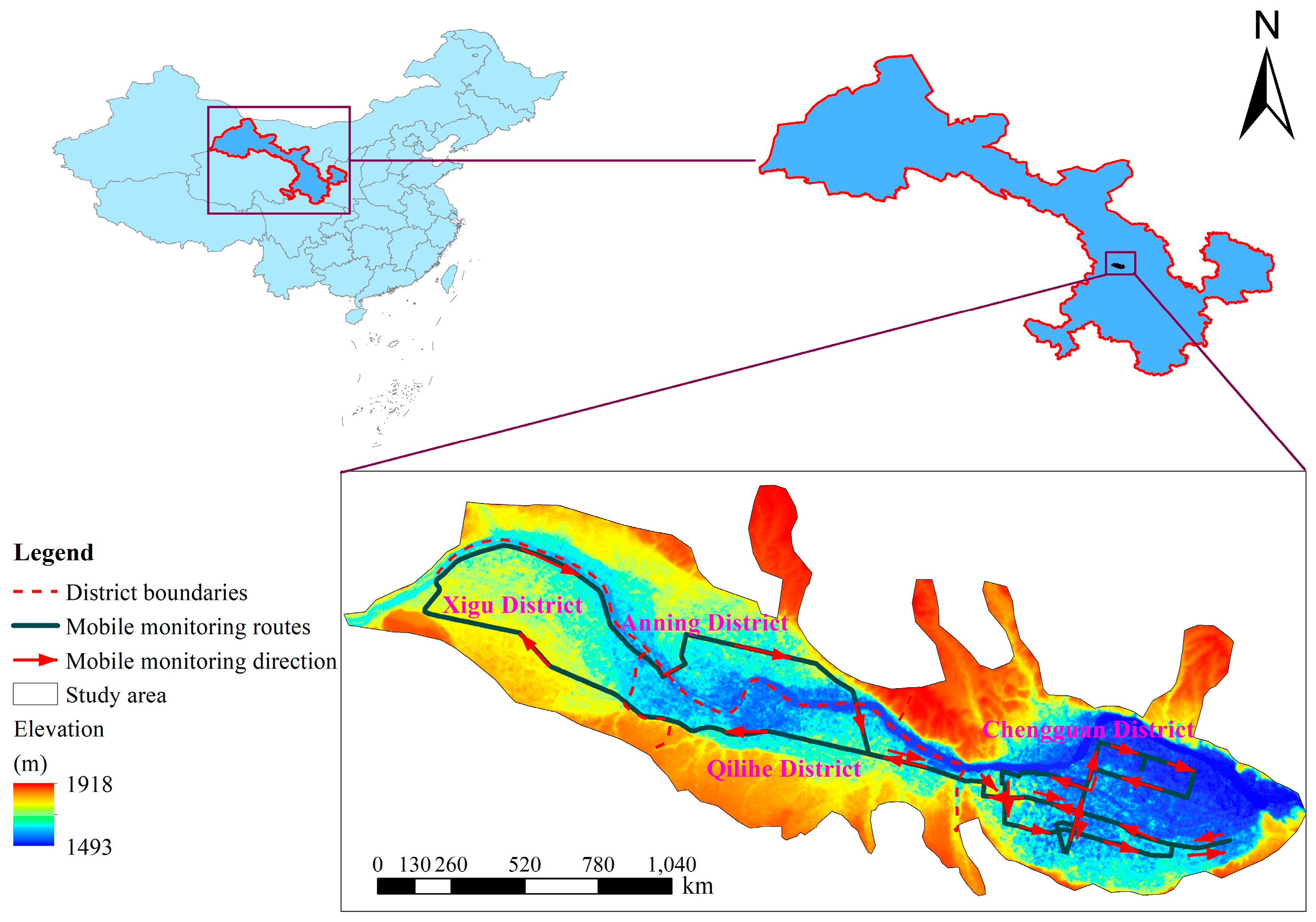
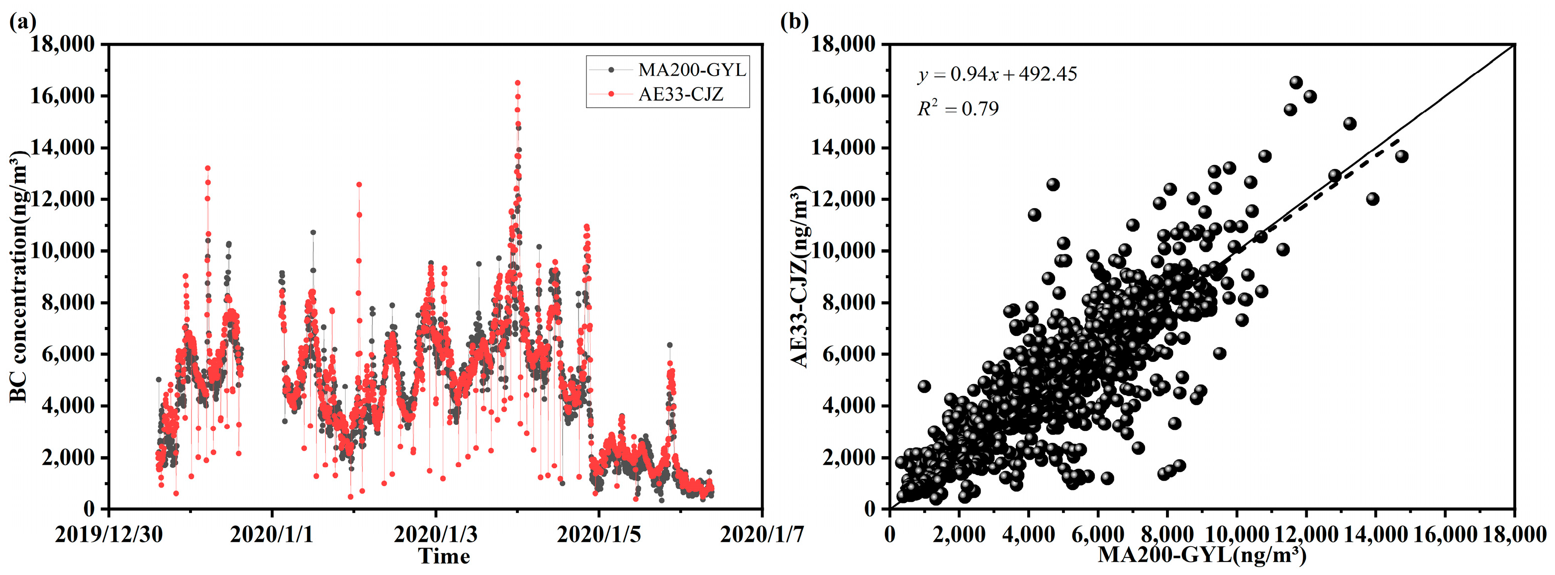
2.1. Mobile Monitoring Campaign

Mobile monitoring campaigns were conducted between 8 and 17 January 2020. To avoid rush hour in the morning, the campaign was designed to start at approximately 9:00 a.m. and end at approximately 2:00 p.m. During this period, the total traffic volume for each road type remained relatively stable. The total length of the designed sampling route was approximately 110 km and the average speed was approximately 25 km/h to yield sufficient data points. The sampling instruments were fixed to the vehicle, and a complete mobile monitoring campaign was conducted daily along the designed monitoring route, as described in our previous study. All sampling sessions were conducted on non-rainy days to avoid interference from instrument electronics and aerosol washout. Before each data collection session, time synchronisation, flow calibration, and full preheating were performed.
In our study, a microAeth MA200 (AethLabs, San Francisco, CA, USA) was used to measure BC concentration. The microAeth MA200 provides real-time loading compensation using dual-spot technology that eliminates the need for correction for filter loading [17]. The instrument has five analytical channels each operating at a different wavelength (880 nm, 625 nm, 528 nm, 470 nm, and 375 nm). Measurement at 880 nm is interpreted as concentration of BC. The optical attenuation (ATN) due to the absorbance of particles collected on the spot is measured. With the gradual accumulation of optically absorbing particles, the ATN also increases during the timebase period. It is then converted to a mass concentration of BC expressed in nanograms per cubic meter (ng/m3) using the known optical absorbance per unit mass of BC material. In this study, the microAeth MA200 was operated with a flow rate of 150 mL/min and temporal resolution of 5 s. Raw BC data were preprocessed to reduce noise using the optimized noise reduction averaging (ONA) algorithm [45].
A Grimm Aerosol Spectrometer (Model 11-D; Grimm Aerosol Technik, Hamburg, Germany) was used to measure the PNC. The instrument works on the principle of scattered light measurement on individual particles and it can perform automatic altitude correction; the monitor can directly measure PNC spectrum distribution in the 0.25 to 35.15 µm size range with 31 channels. In this study, PNC is the sum of the particle number concentrations measured by the 31 channels. The instrument operates at a constant volumetric flow rate of 1.2 L/min and a time resolution of 5 s.
The instrument performance was tested before the mobile monitoring campaigns from 30 December 2019 to 6 January 2020. The microAeth MA200 was placed on the roof of the Guanyun Building of Lanzhou University for sampling. A comparison with the AE33 in the Lanzhou Atmospheric Components Monitoring Superstation (LZU_superstation) during the same period showed that there is a strong linear correlation between MA200 and AE33, with an R2 of 0.79, proving that the MA200 is a reliable instrument and that the data collected through it for mobile monitoring are highly credible (Figure 1).
In addition, the mobile platform was equipped with a portable instrument (UniStrong A5) that used the Beidou Navigation Satellite System (BDS) as the core for accurate positioning. It collected the time, altitude, latitude, and longitude with the resolution of 5 s. Moreover, the air temperature, relative humidity, and air pressure were simultaneously monitored with a 6 s resolution by a data logger (UT330 model).
To evaluate the reliability and stability of portable instruments for mobile monitoring, observations from the LZU_superstation were also used. LZU_superstation, located on the campus of Lanzhou University, has been built and has started observations in 2019. There was a distance of 200 m between the locations of the LZU_superstation and the Guanyun Building for portable instruments. The height of the latter was approximately 40 m higher than that of the former. The LZU_superstation consists of an ambient air quality monitoring system, a particulate matter component monitoring system, a photochemical pollution observation system, and a ground-based remote sensing observation system. It provides rich data support for regional air pollution control, management decisions, and heavy pollution weather warnings and forecasting.
Air pollutant concentrations obtained by mobile monitoring are easily affected by the actual situation of the route. Previous studies have shown that the peak PNC induced by traffic intersections or emitted by vehicles at pedestrian crossings is one order of magnitude higher than the average level on typical roadsides [46,47]. Therefore, situations such as location, stopping time, and starting time occurred when traffic lights or traffic jams were recorded during sampling. Similar to our previous study, some values should be removed before building the LUR model once one of the following situations is met: (1) Monitoring data while waiting for traffic lights according to observation records. (2) The peak is caused by the mobile monitoring vehicle stopping for a long time, exceeding 200 s, at intersections or on congested roads. (3) Some spikes induced by the construction site, cement plant, or freight trucks approached the mobile monitoring instruments. As a final data processing step, temporal or spatial smoothing is often applied to reduce variations due to changes in the atmosphere or display trends more effectively. The types of spatial smoothing include calculating the median or mean values along fixed-length intervals of the route or within a fixed radius of the locations of interest [21]. The models generally performed better for median concentrations than for mean concentrations [48]. The instrument performance testing was performed in IDL 8.5 and spatial smoothing of monitoring data was performed in ArcGIS 10.2.

2.2. Potential Predictor Variables

Five categories of candidate independent variables were assembled to develop the LUR model: road network, land use, land cover, population, and other types. The road network information obtained from the Open Street Map (OSM) dataset included the lengths of all roads, trunk roads, primary roads, secondary roads, tertiary roads, residential roads, unclassified roads, and highways. Land use types were divided into five subcategories: residential, commercial, industrial, transportation station, and public. The land cover datasets were aggregated into eight groups for modelling: cropland, forest, grassland, shrubland, wetland, water, impervious surfaces, and bare land. The population size was obtained by estimating the total number of people in each grid cell. Other types include points of interest (POI_restaurants), elevation, temperature, relative humidity, distance from water bodies, and industrial points in the study area. All potential predictor variables, along with the units and anticipated directions of effects, are summarised in Table A1.
Furthermore, road segments were established along the monitoring route to aggregate mobile monitoring data. This study’s monitored sections were first divided according to the traffic lights and intersections. Road segments beyond 1500 m were divided by an equal distance of 500 m to obtain more samples. A total of 155 road segments were obtained. The shortest and longest segments were 89.61 m and 1289.39 m, respectively. The average length of the road segments was 538.49 m. The number of mobile monitoring data distributed on the road segments varied from 10 to 401, with an average of 107 data aggregates on each road segment. The number of data aggregates on a road segment was generally proportional to the length of the road segment, and the average value of all data on the road segment was aggregated at the midpoint of the road segment.
The variables were either point estimates at a specific location or based on buffers around the measurement location [48]. To explore the affected range of BC and PNC, this study considered the midpoint of each road segment as the centre of the circle to establish different buffers, and the buffer radii were set as 30 m, 50 m, 100 m, 200 m, 300 m, 400 m, 500 m, 1000 m, 2000 m, 3000 m, 4000 m, and 5000 m. The length of different road types, the surface area of land use and land cover types, the total population, the number of POI_restaurants points, and the mean values of meteorological elements (temperature and relative humidity) were calculated in buffers of different radii. The elevation value of the middle point of each road segment, the distance between the middle point and the Yellow River, and the industrial point were calculated. Table 1 shows the data sources and time of the potential predictor variables in this study. The identification and further processing of geographic information was based on ArcGIS 10.2.

2.3. LUR Model Development

This study used the median PNC and BC concentrations on each road segment as dependent variables in the LUR model. The values of the potential independent variables mentioned in Section 2.3 and the median values of PNC and BC were assigned to the midpoint of each road segment. The aggregated dataset of 155 road segments was randomly divided into two groups: A training dataset of 80% and a testing dataset of 20%. The training dataset was used to develop the LUR models for PNC and BC, whereas the testing dataset primarily supported the assessment of model performance.
A supervised stepwise multiple linear regression method was used to select predictors for the LUR models. For each pollutant, the natural logarithm of the aggregated median concentration for each road segment was adopted for the linear regression. First, a univariate regression model was run between the dependent variable and each potential predictor variable, and significant variables at the 95% level (p < 0.05) were identified. Second, the variables with the highest adjusted R2 values for each buffer distance were selected. Third, the selected predictor and dependent variables were processed using stepwise regression to obtain the maximum adjusted R2. As a result, the variable was retained in the model when all of the following conditions were satisfied: (1) each variable had a significant correlation with the dependent variable (p < 0.05), (2) the adjusted R2 of the model increased by more than 1%, (3) the direction of the effect was as expected, (4) the direction of the variables selected in the model did not change, and (5) the variance inflation factor (VIF) of all variables was less than 5 to avoid multicollinearity. Finally, the entire study area was divided into 24,025 100 m × 100 m grids, and the LUR models were applied to predict pollutant concentrations for the centroid location at each grid [19]. In this study, models were built using SPSS, and ArcGIS 10.2 was used to identify the geographic variables and map the predicted PNC and BC.

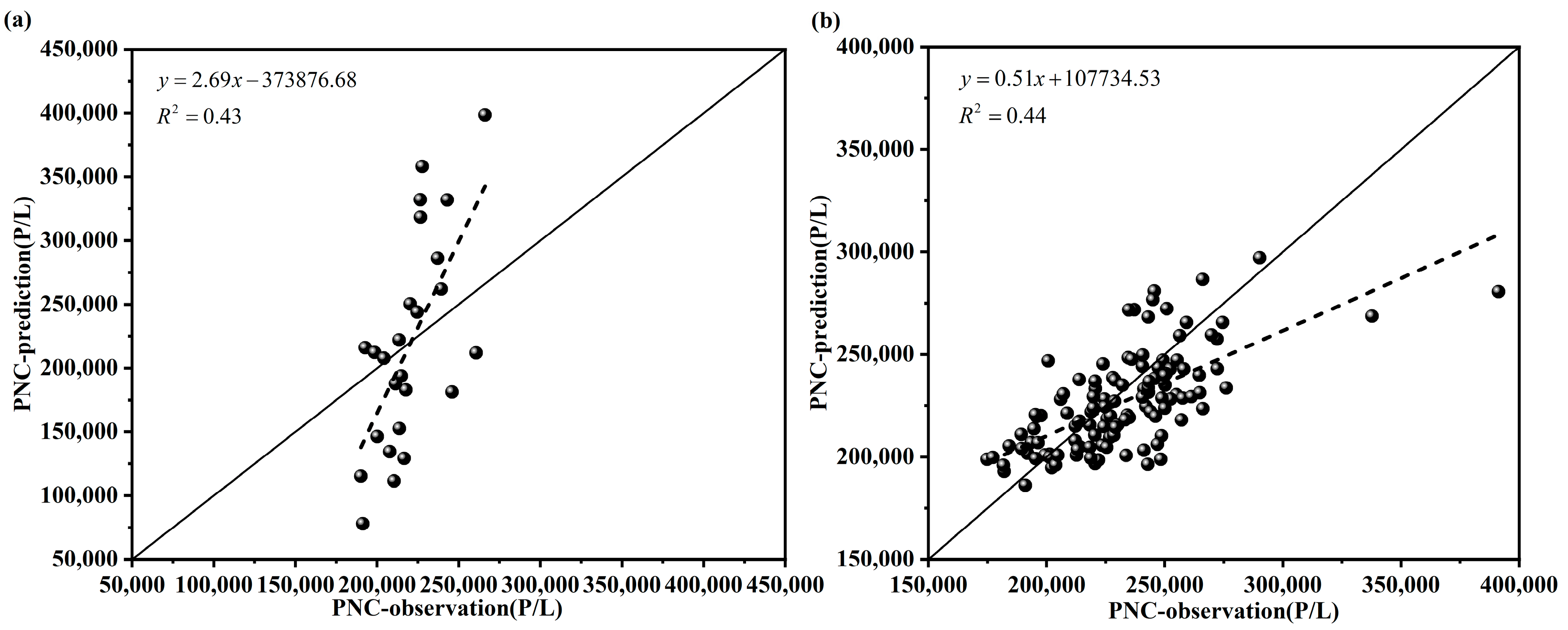
2.4. Model Evaluation

The adjusted R2, R2, and root mean square error (RMSE) are typically used to evaluate the performance of LUR models. The adjusted R2 is an important indicator for measuring the model’s goodness; the larger the adjusted R2, the better the model performance. Certainly, the limited monitoring data and many variables increased the risk of “overfitting” the LUR models [26]. As a result, models were evaluated using hold-out validation (HV) and leave-one-out cross-validation (LOOCV) procedures. R2 can be used to measure prediction accuracy and explains the variation based on spatial or temporal comparisons of average predictions versus observations [1]. Adopted as the decisive criterion of model performance in many air pollution studies, RMSE expresses the difference between the predicted and measured concentrations [39,49]. Therefore, the R2 and RMSE values of the observed and predicted values were calculated using two cross-validation procedures. This study conducted HVs between the predicted concentration and test dataset, which was not used to develop the LUR models. The LOOCV was performed using only the training dataset. Each location used for the LUR model development was omitted, and the model was refitted under the same predictors in the final LUR model. The coefficients were obtained to predict the concentration at the left-out location. This process was repeated 123 times for each model. Calculations related to model evaluation were performed based on IDL 8.5.

3. Results and Discussion

3.1. Results

3.1.1. LUR Model

A summary of the LUR models and validation results for PNC and BC are listed in Table 2. The results showed that six variables were statistically significant predictors of PNC variability: distance from the water body, area of commercial land within a 5000 m circular buffer, length of tertiary roads within a 5000 m circular buffer, area of industrial land within a 5000 m circular buffer, area of public management service land within a 750 m circular buffer, and length of trunk roads within a 750 m circular buffer. The distance from the water body was selected as the first predictor for entering our LUR model for PNC; this showed that water bodies seemed to play an active role in the PNC in the study region. It is well known that the main sources of PNC are traffic-related combustion processes, industrial sources, home heating, and biomass burning. This study’s LUR model of PNC contained two traffic predictors and one industry predictor.
Furthermore, the inclusion of tertiary_5000m and Industrial_5000m increase the explanatory power of the LUR model by 8.6% and 3.5%, respectively. This indicates the major impact of traffic and industrial processes. This is consistent with the conclusion of previous studies that industrial and transportation emissions could be important sources of PNC [50,51]. However, there is significant heterogeneity in the specific emission sources and industries between cities. Commercial land was also predictive of PNC, but in a negative direction.
The sources and dispersion of PNC and BC were different, and the LUR models for BC, including the different predictors, were also different from those for PNC. The LUR model for BC consisted of six predictors, including one traffic predictor. The results showed that 66.7% of the selected variables were land-cover-related, suggesting a substantial contribution of land cover types to improving the environmental BC concentration. In particular, croplands, grasslands, and shrublands accounted for the most adjusted R2. In addition, the model contained one predictor for the number of POI_restaurants in a distant vicinity (5000 m). This indicates the importance of cooking in restaurants. An association between a larger grassland area, shrubland area and water bodies with lower BC concentrations was found, revealing that surrounding greenness and water bodies can mitigate the neighbourhood BC magnitude. In contrast, the associations between other selected variables and BC concentration were positive.
The adjusted R2 of the LUR model for PNC was 0.51, whereas that for BC was slightly higher, at 0.53. The cross-validation metrics indicated that the final prediction model performed modestly. The HV R2 values are 8% and 11% lower than the model-adjusted R2. The LOOCV R2 values for PNC and BC were 7% and 3% lower than the model-adjusted R2. Although the HV results were slightly worse than those of LOOCV, the R2 differences between the models and the above two validation methods were less than 15%, indicating that the models were stable [52]. Figure 2 shows the scatter plots of the predictions and observations of the PNC from HV and LOOCV. The HV R2 and RMSE of PNC were 0.43 and 70,297.93 P/L, respectively. The LOOCV R2 and RMSE of PNC were 0.44 and 23,284.94 P/L, respectively. The HV R2 and RMSE of BC shown in Figure 3 were 0.42 and 801.32 ng/m3, respectively. The LOOCV R2 and RMSE of BC were 0.50 and 886.62 ng/m3, respectively.

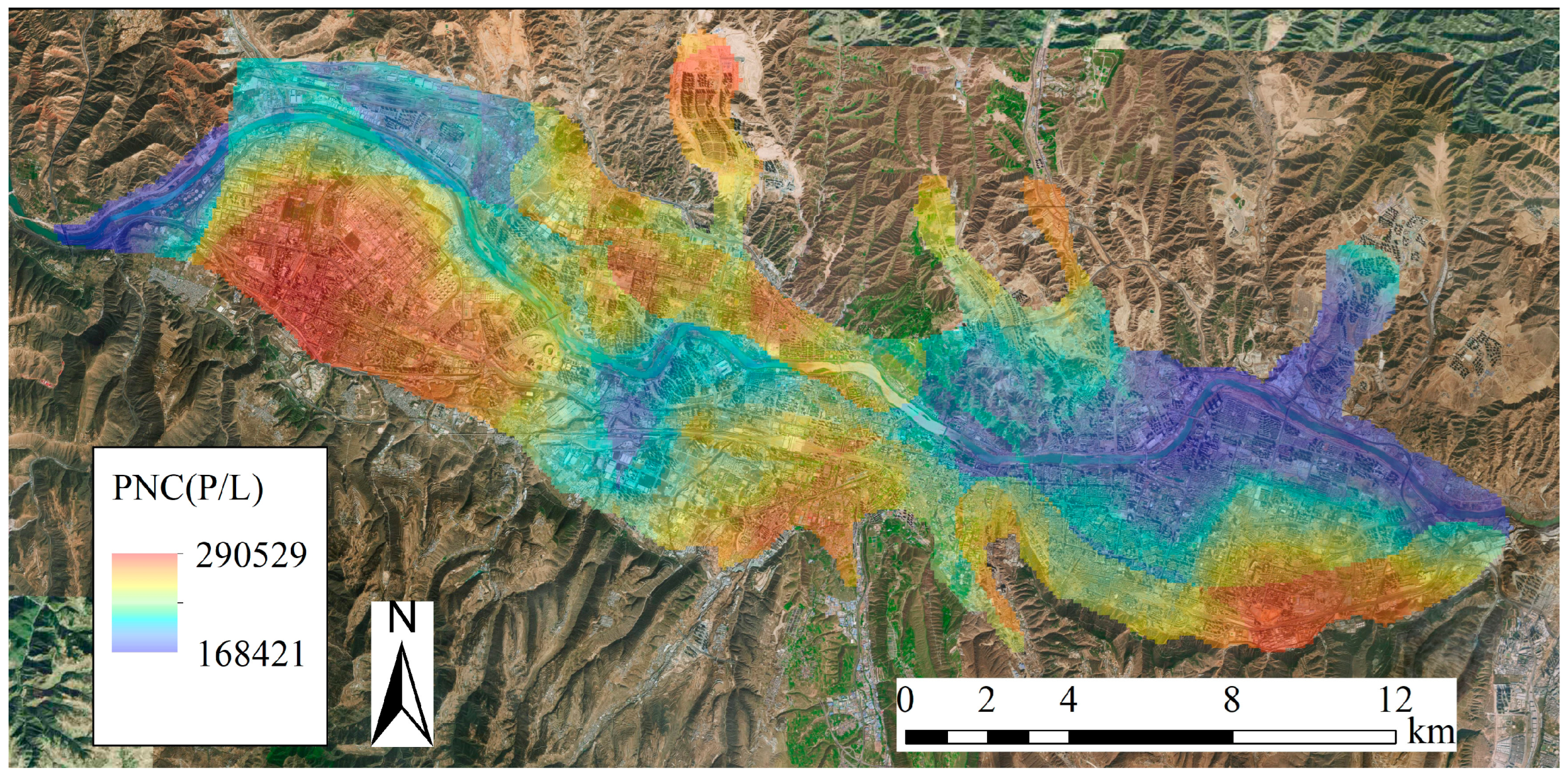
3.1.2. Spatial Distribution of Pollutant Concentrations

As shown in Figure 4, the spatial distribution of the predicted PNC was closely associated with the distance from the water bodies. PNC generally appears at low concentrations along the Yellow River Valley and its adjacent areas. The microclimate formed in the area of the water bodies contributed to the improved air quality and the deposition of particulate matter. In addition, PNC is related to industrial pollution in our LUR model; the largest petrochemical enterprise is in the Xigu District. The Chengguan District, a developed area in the Lanzhou City Centre, has a high population density and a well-developed road network. Thus, traffic emissions are the main source of urban PNC.
Figure 5 shows the spatial distribution of the predicted BC concentrations in Lanzhou. In general, the BC concentration gradually decreased from south to north. High BC concentrations were mainly in the southeastern Xigu, southern Qilihe, and Chengguan Districts. Among the four districts, the Anning District had the lowest BC concentration. Most of the low BC concentration in Anning District was due to the large coverage area of grassland, which had a significant improvement effect. However, there are many freight distribution centres in the Chengguan District, and it is frequently used by large trucks. In the south of Qilihe District, large coal-fired power plants may have a significant impact.

3.2. Discussion

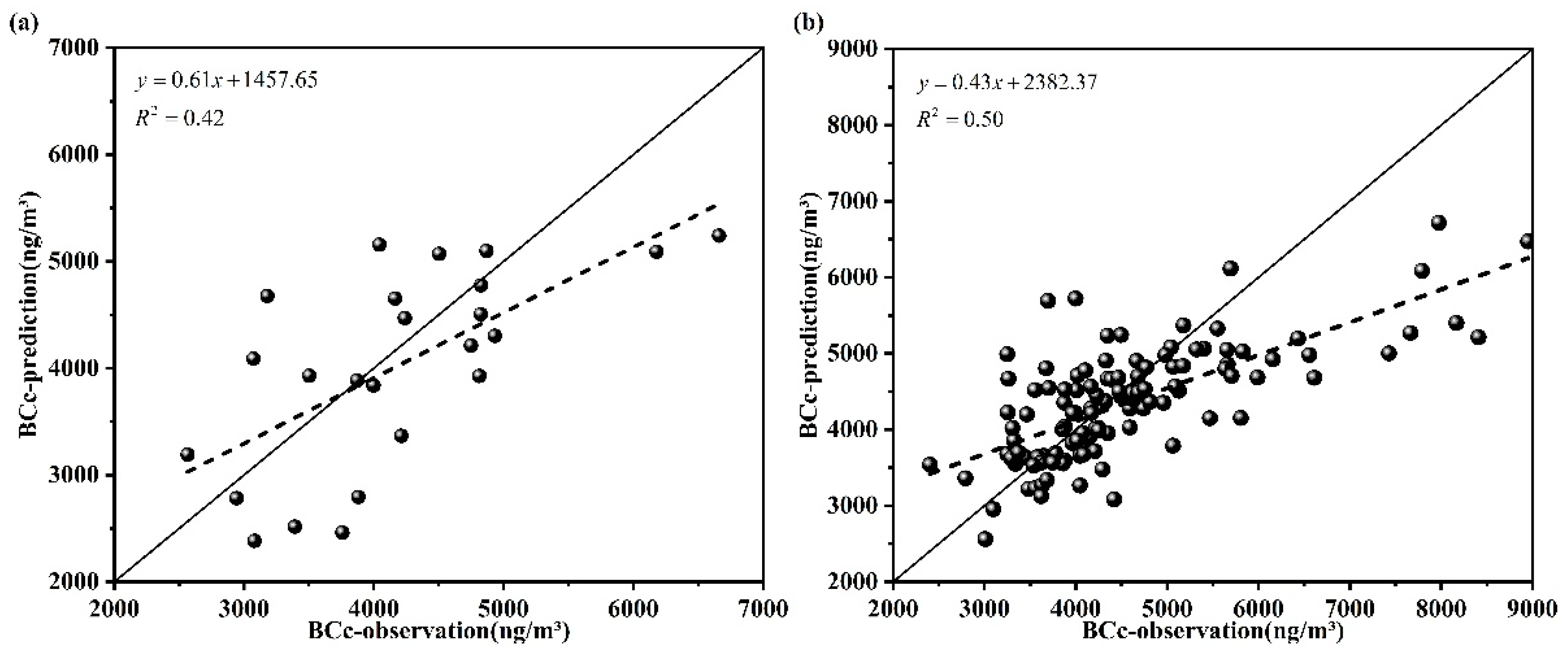
3.2.1. Comparison of Predicted Concentration and the Fixed Station Observation

Comparing the predicted PNC and that observed at the LZU_superstation, the LUR model predicted that the PNC in the main urban area of Lanzhou ranged from 168,421 to 290,529 P/L, and the predicted PNC in the location near the LZU_superstation was approximately 215,400 P/L. During the mobile monitoring period, the PNC in the LZU_superstation ranged from 97,646 to 374,288 P/L, with an average value of 267,298 P/L. The results showed that the predicted concentration in our LUR model was 19.5% lower than that monitored at the LZU_superstation. Regarding PNC, the concentration monitored by the LZU_superstation spans a wider range than our mobile observations. The predicted BC concentrations range from 2721 to 11,227 ng/m3. The BC concentration near the LZU_superstation was approximately 4691 ng/m3. During the mobile monitoring period, the BC concentration at the LZU_superstation ranged from 1503 to 6299 ng/m3, with an average concentration of 3728 ng/m3. The LUR model overestimated the BC concentration compared with the LZU_superstation.
Several previous studies have reported the BC concentrations in Lanzhou. Some studies have claimed that the annual average concentration of BC in Lanzhou ranged from 2000 to 6700 ng/m3 [53,54,55]. Data from the Lanzhou Environmental Protection Bureau building by Tan et al. showed that the average BC concentration in urban areas was 13,800 ng/m3 in the winter of 2012 [56]. Wang et al. reported that BC concentrations in the Xigu and Chengguan Districts were 6700 ng/m3 and 9000 ng/m3, respectively [57]. Comparing the predicted BC concentration in this study and the results of Wang et al., we found that the reason for the difference is that the LUR model was developed using observation data in winter [57]. Generally, the BC concentration in winter is higher than that in summer because of winter heating; therefore, the annual average concentration is lower than the BC concentration in winter.

3.2.2. Comparison with Previous Mobile Monitoring Studies

Most current studies have been conducted on PNC of less than 100 nm in diameter. For example, Xu et al. obtained a mean winter PNC of 2.2 × 10⁷ P/L in Toronto with an instrument mounted on the Urban Scanner [58]. In the greater Seattle area, Blanco et al. obtained PNC ranging from 3.80 to 9.32 × 10⁶ P/L with a hybrid vehicle mobile monitoring [5]. Using two Google Street View cars, Gani et al. obtained PNC from 0.2 to 3.1 × 10⁷ P/L, with a mean value of 1.2 × 10⁷ P/L [59]. Liu et al. monitored PNC of 1.02 × 10⁷ P/L with a range of 10–1000 nm in diameter in Augsburg by walking from November to April 2018 to 2020 [32] and, on 22–25 November 2018, they detected PNC in Bayerisch Eisenstein and Zelezna Ruda at 4.19 × 10⁶ P/L and 5.02 × 10⁶ P/L [31], respectively. In this study, the PNC measurements range from 0.25 to 35.15 µm in diameter. According to the shape of particle number size distribution, the PNC decreases sharply as the particle diameter increases, and the percentage of fine particles (diameter less than 1 µm) accounts for most of the total PNC [60]. Hence, the PNC obtained in this study would be much smaller than the results of previous studies.
Many studies have used mobile observations to measure BC concentrations. Several studies collected BC concentrations during the non-heating period, with their results generally lower than those of this study [61,62]. For example, the BC concentration collected by Liu et al. during the heating period in Germany was lower than our results [31,32]. In the studies by Hove et al. and Talaat et al., although they included both heating and non-heating periods, both collected higher overall BC concentrations than in this study [41,63], indicating that different countries vary greatly in pollutant levels. Even in China, the differences in BC concentration levels between regions are obvious; for example, the mean BC concentration in Taiyuan during the heating period was 4720 ng/m3, with a median of 4540 ng/m3 [43]. However, in Shanghai, the range of BC concentrations during the heating period was 5110–21,880 ng/m3, with an average value of 10,770 ng/m3 [44]. Our LUR model predicted BC concentrations ranging from 2720 to 11,230 ng/m3, generally higher than those of foreign studies. This may be because there are more sources of BC pollution in Lanzhou than in most other cities, resulting in higher measured concentrations and affecting the predicted values.

3.2.3. Comparison of Model Performance

In this study, the adjusted R2 of the LUR model of PNC was 0.51, the R2 of HV was 0.43, the R2 of LOOCV was 0.44, and the difference between the R2 values obtained using the two cross-validation methods was small. Saha et al. used the PNC data obtained from 38 sites in the national PNC dataset in the United States to build the LUR model of PNC with an R2 of 0.77, and the R2 of random 10-fold HV was 0.72 [64]. Chang et al. developed LUR models for PNC at size ranges of <0.5 μm, 0.5–1 μm, 1–2.5 μm, 2.5–10 μm, and ≥10 μm based on 50 particulate concentration monitoring sites in the metropolitan area of Taichung. The results showed adjusted R2 of 0.28–0.44 for the LUR models and R2 of 0.27–0.41 for LOOCV. They indicated that, the smaller the difference between the LOOCV R2 of model and R2, the better the model works [65]. The model performance of our PNC was similar to that of London, which used PNC data with a range of 10–1000 nm from 120 sites with an adjusted R2 of 0.59, and the R2 of HV was 0.44 [66]. Overall, the performance of the LUR model for PNC in this study was moderate.
The adjusted R2 of the LUR model for BC was 0.53, the R2 of HV was 0.42, and the R2 of LOOCV was 0.50. The HV result was slightly worse than the LOOCV result; however, its overall performance was better than that of the PNC model. The performance of our model was better than that of most studies. Xu et al. built seasonal LUR models for Taiyuan, with an adjusted R2 of 0.48 for the model and 0.47 for LOOCV [43]. Cai et al. built an LUR model for BC in Taizhou with an adjusted R2 of 0.78, and the R2 for LOOCV was lower than approximately 0.08 [19]. Boniardi used the monitored data and measurements from 34 monitoring sites to build a winter LUR model with an adjusted R2 of 0.52 and an R2 of 0.35 LOOCV [39]. We used a similar modelling method as Liu et al. [44]; however, the model they built for BC in Shanghai worked better than that of this study, with an adjusted R2 of 0.67 and LOOCV of 0.66. Compared with the above studies, the BC model obtained in this study performed better.

3.2.4. Variables of the PNC and BC Models

Traffic-related variables were the most common predictors in PNC and BC models, all of which incorporated at least one road variable in the LUR models [51,66,67], as does the model in this study, which, for PNC, included the length of tertiary roads in 5000 m buffers and the length of primary roads in 2000 m buffers, while the BC model included the length of primary roads in 2000 m buffers. The industrial land area was another common predictor in our model, as well as in the PNC models used in other studies [19,67]. The BC LUR model in this study, built by Cai et al. and Xu et al., contained the independent variable of croplands [19,43]. In summary, our model was partly similar to other studies, differing in that the other models contained variables related to meteorological elements and buildings, which were not included in the pre-selected independent variables in this study. Variables related to water bodies (areas of the water bodies or distance from the water bodies) were another common category of predictors incorporated into the two models in this study. Because the entire urban area of Lanzhou is located within the valley, and the Yellow River flows through the centre of the city within the valley, the Yellow River channel is a ventilation channel relative to the high-rise buildings on both sides of the river, which is conducive to the outwards diffusion of pollutants within the valley. The ones that entered the model were larger buffers (1000–5000 m); the 2000 m and 5000 m buffers were the most common.

3.2.5. Limitations

Because the construction cost of fixed stations is too high, there was only one fixed station, including the PNC and BC measurements, for the reference data in this study for the time trend adjusted for the mobile monitoring dataset. Although Lanzhou belongs to a narrow region with an east–west distance of approximately 30 km, the time trend revision based on one reference point is not sufficiently representative; therefore, this study did not adjust the time trend for PNC and BC. Given the high construction cost of fixed stations, the use of low-cost portable instruments, such as Model 11-D and microAeth MA200, in future work will be deployed at multiple locations to complement mobile monitoring.
In addition, the unexplained variability in the study may be related to the untimely updated information of the independent variables, such as land cover/land use and population density. With the rapid urban development in recent years, the untimely updated information of each variable may greatly impact the final model. Moreover, we will use higher-resolution information to improve the accuracy of the models in predicting pollutant concentrations.
Finally, some studies indicated that building-related predictors were introduced in some models, which enhanced their explanatory capability and even had the highest explanatory power. The complex layout of dense buildings and streets can lead to changes in airflow that affect the spatial variation of pollutants in large cities [26,43]. However, this study did not introduce building-related variables and needs improvement in future studies.

4. Conclusions

In this study, LUR models for PNC and BC were developed based on a short-term mobile monitoring campaign in the urban area of Lanzhou from 8 to 17 January 2020. The adjusted R2 of the LUR models were 0.51 and 0.53 for PNC and BC, respectively. Subsequently, LOOCV and HV were performed for both models. For the PNC model, the R2 of LOOCV was 0.44 and the RMSE was 23,285 P/L, while the R2 and RMSE of HV were 0.43 and 70,298 P/L, respectively. For the BC model, the R2 and RMSE of LOOCV were 0.50 and 887 ng/m3, respectively, and the R2 and RMSE of HV were 0.42 and 801 ng/m3, respectively. Overall, the LUR model of PNC performed at a moderate level, and the LUR model of BC performed better.
The spatial distributions of PNC and BC in Lanzhou City were predicted using the LUR models. The spatial distribution of the predicted PNC was closely associated with the distance from the water bodies. PNC generally appears at low concentrations along the Yellow River Valley and its adjacent areas. PNC is related to industrial pollution in our LUR model, and the largest petrochemical enterprise is located in the Xigu District. The BC concentration gradually decreases from south to north. High BC concentrations were mainly found in the southeastern Xigu, southern Qilihe, and Chengguan Districts. This phenomenon may be related to many freight distribution centres in the Chengguan District and the distribution of large coal-fired power plants in the southern Qilihe District. Among the four districts, the Anning District had the lowest BC concentration.
There have been few previous studies on mobile monitoring of air pollutant concentrations in Lanzhou, especially related to LUR models. For PNC, the range of particle sizes was different from most studies, and this study has a much larger particle range to allow a more comprehensive view of the particle situation in Lanzhou. Despite the development of LUR models for PNC and BC, many inadequacies remain, as described in the limitations Section 3.2.5. However, there have been few studies on the spatial prediction of PNC and BC in Lanzhou before this, and this study helps to determine the level of risk that air pollutants pose to human health by predicting the spatial distribution of air pollutants. Moreover, this modeling method based on low-cost portable sampling instruments in this paper can be more easily extended to more cities to achieve spatial prediction of air pollutants. This study provides an important basis for developing seasonal and more advanced air pollutant prediction models in city areas. It provides an opportunity to explore the effects of the fine-scale distribution of air pollution on population health. In the next study, long-term research will be conducted for a variety of air pollutants to optimize the model effect as much as possible by increasing the types of independent variables and exploring some advanced modeling methods, among other things, to provide a reliable basis for exposure assessment.

Author Contributions

Conceptualization, T.Z.; methodology, T.Z. and S.F.; software, S.F.; validation, T.Z.; formal analysis, T.Z. and S.F.; investigation, T.Z., S.F., L.J., X.Z., X.L., X.S. and Y.W.; resources, T.Z.; data curation, T.Z., S.F., L.J., X.Z., X.L., X.S. and Y.W.; writing—original draft preparation, T.Z. and S.F.; writing—review and editing, T.Z., S.F. and L.J.; visualization, S.F.; supervision, T.Z. and L.J.; project administration, T.Z.; funding acquisition, T.Z. All authors have read and agreed to the published version of the manuscript.

Funding

This research was funded by the National Science Foundation of China [41975019]; Gansu Provincial Science and Technology Innovative Talent Program: High-level Talent and Innovative Team Special Project [No. 22JR9KA001]; the Fundamental Research Funds for the Central Universities [lzujbky-2022-kb10]; and the Natural Science Foundation of Gansu Province [22JR5RA441].

Data Availability Statement

The data presented in this study are available upon request from the corresponding author. The data are not publicly available because of the need for future research.

Acknowledgments

We thank the Lanzhou Ecology and Environment Bureau for providing the Lanzhou University superstation measurements. We thank Xiangyu Xu for helpful guidance on model building and acknowledge all anonymous reviewers for their insightful and valuable comments.

Conflicts of Interest

The authors declare no conflict of interest.

Appendix A

Lanzhou is the capital of Gansu Province, an important industrial base and comprehensive transportation hub in northwest China. Moreover, it was previously ranked as the most polluted city among the provincial capitals in China, and the main urban areas include the four districts (Chengguan, Qilihe, Xigu, and Anning) shown in Figure A1. Mountains to the south and north surround the Lanzhou city core, a typical valley city, extending mainly from east to west and approximately 40 km long; the narrowest width from north to south is approximately 3 km [68]. Overall, the city’s shape is similar to that of a saddle city. The four small tails on the northern side of the city can be found because of the urban expansion in recent years, where there are also many resident populations after whittling down mountains and building buildings. The mean elevation of Lanzhou is 1500 m. The city is high in the west and south and low in the northeast, covering a total area of 13,100 km2, with a population of 4.42 million at the end of 2022. The Yellow River runs through the city from west to east. Annual rainfall is 327.7 mm, and the average temperature is 9.3 °C in Lanzhou [69]. Spring and winter are the dust-dominated periods in Lanzhou [70].
Figure A1. Location of Lanzhou and topography.
Sustainability 15 12828 g0a1
Table A1. Summary of potential predictor variables.
CategoriesPredictor VariablesDescriptionUnitAnticipated Directions
Road NetworkRoadlengthLength of all roadsm+
TrunkLength of the trunk roadsm+
PrimaryLength of the primary roadsm+
SecondaryLength of secondary roadsm+
TertiaryLength of tertiary roadsm+
ResidentialLength of residential roadsm+
OTRLength of unclassified roadsm+
MotorLength of highwaysm+
Land UseResidentialArea of residential and village landkm2/
CommercialArea of business and commercial landkm2/
IndustrialArea of industrial landkm2+
Transportation stationsArea of land for transportation facilitieskm2+
PublicArea of public building landkm2/
Land CoverCroplandArea of agricultural landm2/
ForestArea of forested landm2-
GrasslandArea of grassm2-
ShrublandArea of shrublandm2/
WetlandArea of wetlandm2/
WaterArea of all water bodiesm2-
Impervious surfaceArea of impermeable surfacem2/
BarelandArea of barelandm2/
Population Number of populationcount+
Other TypesPOI_restaurantsNumber of restaurantscount+
ElevationElevation of the midpoint of road segmentm/
TemperatureSurface temperature°C/
Relative humiditySurface relative humidity /
Dist waterDistance from the nearest water bodiesm/
Dist pointDistance from the nearest industrial emission pointm/

References

  1. Kirwa, K.; Szpiro, A.A.; Sheppard, L.; Sampson, P.D.; Wang, M.; Keller, J.P.; Young, M.T.; Kim, S.-Y.; Larson, T.V.; Kaufman, J.D. Fine-Scale Air Pollution Models for Epidemiologic Research: Insights from Approaches Developed in the Multi-ethnic Study of Atherosclerosis and Air Pollution (MESA Air). Curr. Environ. Health Rep. 2021, 8, 113–126. [Google Scholar] [CrossRef]
  2. Jin, L.; Zhou, T.; Fang, S.; Zhou, X.; Bai, Y. Association of air pollutants and hospital admissions for respiratory diseases in Lanzhou, China, 2014–2019. Environ. Geochem. Health 2022, 45, 941–959. [Google Scholar] [CrossRef] [PubMed]
  3. Gozzi, F.; Della Ventura, G.; Marcelli, A. Mobile monitoring of particulate matter: State of art and perspectives. Atmos. Pollut. Res. 2016, 7, 228–234. [Google Scholar] [CrossRef]
  4. Xu, X.; Ha, S.U.; Basnet, R. A Review of Epidemiological Research on Adverse Neurological Effects of Exposure to Ambient Air Pollution. Front. Public Health 2016, 4, 157. [Google Scholar] [CrossRef]
  5. Blanco, M.N.; Bi, J.; Austin, E.; Larson, T.V.; Marshall, J.D.; Sheppard, L. Impact of Mobile Monitoring Network Design on Air Pollution Exposure Assessment Models. Environ. Sci. Technol. 2023, 57, 440–450. [Google Scholar] [CrossRef] [PubMed]
  6. Leitte, A.M.; Schlink, U.; Herbarth, O.; Wiedensohler, A.; Pan, X.-C.; Hu, M.; Wehner, B.; Breitner, S.; Peters, A.; Wichmann, H.E.; et al. Associations between size-segregated particle number concentrations and respiratory mortality in Beijing, China. Int. J. Environ. Health Res. 2012, 22, 119–133. [Google Scholar] [CrossRef]
  7. Breitner, S.; Liu, L.; Cyrys, J.; Brueske, I.; Franck, U.; Schlink, U.; Leitte, A.M.; Herbarth, O.; Wiedensohler, A.; Wehner, B.; et al. Sub-micrometer particulate air pollution and cardiovascular mortality in Beijing, China. Sci. Total Environ. 2011, 409, 5196–5204. [Google Scholar] [CrossRef]
  8. Dons, E.; Int Panis, L.; Van Poppel, M.; Theunis, J.; Wets, G. Personal exposure to Black Carbon in transport microenvironments. Atmos. Environ. 2012, 55, 392–398. [Google Scholar] [CrossRef]
  9. Wang, Y.; Li, X.; Shi, Z.; Huang, L.; Li, J.; Zhang, H.; Ying, Q.; Wang, M.; Ding, D.; Zhang, X.; et al. Premature Mortality Associated with Exposure to Outdoor Black Carbon and Its Source Contributions in China. Resour. Conserv. Recycl. 2021, 170, 105620. [Google Scholar] [CrossRef]
  10. Liu, S.; Huang, Q.; Chen, C.; Song, Y.; Zhang, X.; Dong, W.; Zhang, W.; Zhao, B.; Nan, B.; Zhang, J.; et al. Joint effect of indoor size-fractioned particulate matters and black carbon on cardiopulmonary function and relevant metabolic mechanism: A panel study among school children. Environ. Pollut. 2022, 307, 119533. [Google Scholar] [CrossRef]
  11. Smith, K.R.; Jerrett, M.; Anderson, H.R.; Burnett, R.T.; Stone, V.; Derwent, R.; Atkinson, R.W.; Cohen, A.; Shonkoff, S.B.; Krewski, D.; et al. Health and Climate Change 5 Public health benefits of strategies to reduce greenhouse-gas emissions: Health implications of short-lived greenhouse pollutants. Lancet 2009, 374, 2091–2103. [Google Scholar] [CrossRef] [PubMed]
  12. Geng, F.; Hua, J.; Mu, Z.; Peng, L.; Xu, X.; Chen, R.; Kan, H. Differentiating the associations of black carbon and fine particle with daily mortality in a Chinese city. Environ. Res. 2013, 120, 27–32. [Google Scholar] [CrossRef] [PubMed]
  13. Rahmatinia, M.; Hadei, M.; Hopke, P.K.; Querol, X.; Shahsavani, A.; Namvar, Z.; Kermani, M. Relationship between ambient black carbon and daily mortality in Tehran, Iran: A distributed lag nonlinear time series analysis. J. Environ. Health Sci. Eng. 2021, 19, 907–916. [Google Scholar] [CrossRef]
  14. Szozda, R. Pneumoconiosis in carbon black workers. J. UOEH 1996, 18, 223–228. [Google Scholar] [CrossRef]
  15. Wang, S.; Wu, G.; Du, Z.; Wu, W.; Ju, X.; Yimaer, W.; Chen, S.; Zhang, Y.; Li, J.; Zhang, W.; et al. The causal links between long-term exposure to major PM2.5 components and the burden of tuberculosis in China. Sci. Total Environ. 2023, 870, 161745. [Google Scholar] [CrossRef]
  16. Sun, Y.; Yang, T.; Gui, H.; Li, X.; Wang, W.; Duan, J.; Mao, S.; Yin, H.; Zhou, B.; Lang, J.; et al. Atmospheric environment monitoring technology and equipment in China: A review and outlook. J. Environ. Sci. 2023, 123, 41–53. [Google Scholar] [CrossRef]
  17. Xiang, S.; Zhang, S.; Wang, H.; Wen, Y.; Yu, Y.T.; Li, Z.; Wallington, T.J.; Shen, W.; Deng, Y.; Tan, Q.; et al. Mobile Measurements of Carbonaceous Aerosol in Microenvironments to Discern Contributions from Traffic and Solid Fuel Burning. Environ. Sci. Technol. Lett. 2021, 8, 867–872. [Google Scholar] [CrossRef]
  18. Yeom, K. Development of urban air monitoring with high spatial resolution using mobile vehicle sensors. Environ. Monit. Assess. 2021, 193, 375. [Google Scholar] [CrossRef]
  19. Cai, J.; Ge, Y.; Li, H.; Yang, C.; Liu, C.; Meng, X.; Wang, W.; Niu, C.; Kan, L.; Schikowski, T.; et al. Application of land use regression to assess exposure and identify potential sources in PM2.5, BC, NO2 concentrations. Atmos. Environ. 2020, 223, 117267. [Google Scholar] [CrossRef]
  20. Birmili, W.; Rehn, J.; Vogel, A.; Boehlke, C.; Weber, K.; Rasch, F. Micro-scale variability of urban particle number and mass concentrations in Leipzig, Germany. Meteorol. Z. 2013, 22, 155–165. [Google Scholar] [CrossRef]
  21. Samad, A.; Vogt, U. Mobile air quality measurements using bicycle to obtain spatial distribution and high temporal resolution in and around the city center of Stuttgart. Atmos. Environ. 2021, 244, 117915. [Google Scholar] [CrossRef]
  22. Wang, Y.; Hopke, P.K.; Utell, M.J. Urban-scale Spatial-temporal Variability of Black Carbon and Winter Residential Wood Combustion Particles. Aerosol Air Qual. Res. 2011, 11, 473–481. [Google Scholar] [CrossRef]
  23. Gulliver, J.; de Hoogh, K.; Hansell, A.; Vienneau, D. Development and Back-Extrapolation of NO2 Land Use Regression Models for Historic Exposure Assessment in Great Britain. Environ. Sci. Technol. 2013, 47, 7804–7811. [Google Scholar] [CrossRef] [PubMed]
  24. Jin, L.; Berman, J.D.; Zhang, Y.; Thurston, G.; Zhang, Y.; Bell, M.L. Land use regression study in Lanzhou, China: A pilot sampling and spatial characteristics of pilot sampling sites. Atmos. Environ. 2019, 210, 253–262. [Google Scholar] [CrossRef]
  25. Briggs, D.J.; Collins, S.; Elliott, P.; Fischer, P.; Kingham, S.; Lebret, E.; Pryl, K.; Van Reeuwijk, H.; Smallbone, K.; Van Der Veen, A. Mapping urban air pollution using GIS: A regression-based approach. Int. J. Geogr. Inf. Sci. 1997, 11, 699–718. [Google Scholar] [CrossRef]
  26. Gillespie, J.; Beverland, I.J.; Hamilton, S.; Padmanabhan, S. Development, Evaluation, and Comparison of Land Use Regression Modeling Methods to Estimate Residential Exposure to Nitrogen Dioxide in a Cohort Study. Environ. Sci. Technol. 2016, 50, 11085–11093. [Google Scholar] [CrossRef] [PubMed]
  27. Ryan, P.H.; LeMasters, G.K. A Review of Land-use Regression Models for Characterizing Intraurban Air Pollution Exposure. Inhal. Toxicol. 2007, 19, 127–133. [Google Scholar] [CrossRef] [PubMed]
  28. Brauer, M.; Hoek, G.; van Vliet, P.; Meliefste, K.; Fischer, P.; Gehring, U.; Heinrich, J.; Cyrys, J.; Bellander, T.; Lewne, M.; et al. Estimating Long-Term Average Particulate Air Pollution Concentrations: Application of Traffic Indicators and Geographic Information Systems. Epidemiology 2003, 14, 228–239. [Google Scholar] [CrossRef]
  29. Zou, B.; Luo, Y.; Wan, N.; Zheng, Z.; Sternberg, T.; Liao, Y. Performance comparison of LUR and OK in PM2.5 concentration mapping: A multidimensional perspective. Sci. Rep. 2015, 5, 8698. [Google Scholar] [CrossRef]
  30. Rahman, M.M.; Karunasinghe, J.; Clifford, S.; Knibbs, L.D.; Morawska, L. New insights into the spatial distribution of particle number concentrations by applying non-parametric land use regression modelling. Sci. Total Environ. 2020, 702, 134708. [Google Scholar] [CrossRef]
  31. Liu, X.; Schnelle-Kreis, J.; Zhang, X.; Bendl, J.; Khedr, M.; Jakobi, G.; Schloter-Hai, B.; Hovorka, J.; Zimmermann, R. Integration of air pollution data collected by mobile measurement to derive a preliminary spatiotemporal air pollution pro file from two neighboring German-Czech border villages. Sci. Total Environ. 2020, 722, 137632. [Google Scholar] [CrossRef] [PubMed]
  32. Liu, X.; Hadiatullah, H.; Khedr, M.; Zhang, X.; Schnelle-Kreis, J.; Zimmermann, R.; Adam, T. Personal exposure to various size fractions of ambient particulate matter during the heating and non-heating periods using mobile monitoring approach: A case study in Augsburg, Germany. Atmos. Pollut. Res. 2022, 13, 101483. [Google Scholar] [CrossRef]
  33. Patton, A.P.; Collins, C.; Naumova, E.N.; Zamore, W.; Brugge, D.; Durant, J.L. An Hourly Regression Model for Ultrafine Particles in a Near-Highway Urban Area. Environ. Sci. Technol. 2014, 48, 3272–3280. [Google Scholar] [CrossRef]
  34. Simon, M.C.; Patton, A.P.; Naumova, E.N.; Levy, J.I.; Kumar, P.; Brugge, D.; Durant, J.L. Combining Measurements from Mobile Monitoring and a Reference Site to Develop Models of Ambient Ultrafine Particle Number Concentration at Residences. Environ. Sci. Technol. 2018, 52, 6985–6995. [Google Scholar] [CrossRef] [PubMed]
  35. Cattani, G.; Gaeta, A.; di Bucchianico, A.D.M.; De Santis, A.; Gaddi, R.; Cusano, M.; Ancona, C.; Badaloni, C.; Forastiere, F.; Gariazzo, C.; et al. Development of land-use regression models for exposure assessment to ultrafine particles in Rome, Italy. Atmos. Environ. 2017, 156, 52–60. [Google Scholar] [CrossRef]
  36. Sabaliauskas, K.; Jeong, C.-H.; Yao, X.; Reali, C.; Sun, T.; Evans, G.J. Development of a land-use regression model for ultrafine particles in Toronto, Canada. Atmos. Environ. 2015, 110, 84–92. [Google Scholar] [CrossRef]
  37. Wolf, K.; Cyrys, J.; Harcinikova, T.; Gu, J.; Kusch, T.; Hampel, R.; Schneider, A.; Peters, A. Land use regression modeling of ultrafine particles, ozone, nitrogen oxides and markers of particulate matter pollution in Augsburg, Germany. Sci. Total Environ. 2017, 579, 1531–1540. [Google Scholar] [CrossRef]
  38. Hoek, G.; Beelen, R.; Kos, G.; Dijkema, M.; van der Zee, S.C.; Fischer, P.H.; Brunekreef, B. Land Use Regression Model for Ultrafine Particles in Amsterdam. Environ. Sci. Technol. 2011, 45, 622–628. [Google Scholar] [CrossRef]
  39. Boniardi, L.; Dons, E.; Campo, L.; Van Poppel, M.; Int Panis, L.; Fustinoni, S. Annual, seasonal, and morning rush hour Land Use Regression models for black carbon in a school catchment area of Milan, Italy. Environ. Res. 2019, 176, 108520. [Google Scholar] [CrossRef]
  40. Kerckhoffs, J.; Hoek, G.; Vlaanderen, J.; van Nunen, E.; Messier, K.; Brunekreef, B.; Gulliver, J.; Vermeulen, R. Robustness of intra urban land-use regression models for ultrafine particles and black carbon based on mobile monitoring. Environ. Res. 2017, 159, 500–508. [Google Scholar] [CrossRef]
  41. Talaat, H.; Xu, J.; Hatzopoulou, M.; Abdelgawad, H. Mobile monitoring and spatial prediction of black carbon in Cairo, Egypt. Environ. Monit. Assess. 2021, 193, 587. [Google Scholar] [CrossRef]
  42. Hankey, S.; Marshall, J.D. On-bicycle exposure to particulate air pollution: Particle number, black carbon, PM2.5, and particle size. Atmos. Environ. 2015, 122, 65–73. [Google Scholar] [CrossRef]
  43. Xu, X.; Qin, N.; Qi, L.; Zou, B.; Cao, S.; Zhang, K.; Yang, Z.; Liu, Y.; Zhang, Y.; Duan, X. Development of season-dependent land use regression models to estimate BC and PM1 exposure. Sci. Total Environ. 2021, 793, 148540. [Google Scholar] [CrossRef]
  44. Liu, M.; Peng, X.; Meng, Z.; Zhou, T.; Long, L.; She, Q. Spatial characteristics and determinants of in-traffic black carbon in Shanghai, China: Combination of mobile monitoring and land use regression model. Sci. Total Environ. 2019, 658, 51–61. [Google Scholar] [CrossRef]
  45. Hagler, G.; Yelverton, T.; Vedantham, R.; Hansen, A.; Turner, J. Post-processing Method to Reduce Noise while Preserving High Time Resolution in Aethalometer Real-time Black Carbon Data. Aerosol Air Qual. Res. 2011, 11, 539–546. [Google Scholar] [CrossRef]
  46. Goel, A.; Kumar, P. A review of fundamental drivers governing the emissions, dispersion and exposure to vehicle-emitted nanoparticles at signalised traffic intersections. Atmos. Environ. 2014, 97, 316–331. [Google Scholar] [CrossRef]
  47. Jayaratne, E.R.; Wang, L.; Heuff, D.; Morawska, L.; Ferreira, L. Increase in particle number emissions from motor vehicles due to interruption of steady traffic flow. Transp. Res. Part D Transp. Environ. 2009, 14, 521–526. [Google Scholar] [CrossRef]
  48. Hankey, S.; Marshall, J.D. Land Use Regression Models of On-Road Particulate Air Pollution (Particle Number, Black Carbon, PM2.5, Particle Size) Using Mobile Monitoring. Environ. Sci. Technol. 2015, 49, 9194–9202. [Google Scholar] [CrossRef] [PubMed]
  49. Tessum, M.W.; Sheppard, L.; Larson, T.V.; Gould, T.R.; Kaufman, J.D.; Vedal, S. Improving Air Pollution Predictions of Long-Term Exposure Using Short-Term Mobile and Stationary Monitoring in Two US Metropolitan Regions. Environ. Sci. Technol. 2021, 55, 3530–3538. [Google Scholar] [CrossRef]
  50. Presto, A.A.; Saha, P.K.; Robinson, A.L. Past, present, and future of ultrafine particle exposures in North America. Atmos. Environ. X 2021, 10, 100109. [Google Scholar] [CrossRef]
  51. Bertazzon, S.; Couloigner, I.; Mirzaei, M. Spatial regression modelling of particulate pollution in Calgary, Canada. GeoJournal 2022, 87, 2141–2157. [Google Scholar] [CrossRef] [PubMed]
  52. Eeftens, M.; Beelen, R.; de Hoogh, K.; Bellander, T.; Cesaroni, G.; Cirach, M.; Declercq, C.; Dedele, A.; Dons, E.; de Nazelle, A.; et al. Development of Land Use Regression Models for PM2.5, PM2.5 Absorbance, PM10 and PMcoarse in 20 European Study Areas; Results of the ESCAPE Project. Environ. Sci. Technol. 2012, 46, 11195–11205. [Google Scholar] [CrossRef] [PubMed]
  53. Zhang, Y.; Kang, S. Characteristics of carbonaceous aerosols analyzed using a multiwavelength thermal/optical carbon analyzer: A case study in Lanzhou City. Sci. China Earth Sci. 2019, 62, 389–402. [Google Scholar] [CrossRef]
  54. Chen, P.; Kang, S.; Gan, Q.; Yu, Y.; Yuan, X.; Liu, Y.; Tripathee, L.; Wang, X.; Li, C. Concentrations and light absorption properties of PM2.5 organic and black carbon based on online measurements in Lanzhou, China. J. Environ. Sci. 2023, 131, 84–95. [Google Scholar] [CrossRef] [PubMed]
  55. Zhang, X.; Li, Z.; Wang, F.; Song, M.; Zhou, X.; Ming, J. Carbonaceous Aerosols in PM1, PM2.5, and PM10 Size Fractions over the Lanzhou City, Northwest China. Atmosphere 2020, 11, 1368. [Google Scholar] [CrossRef]
  56. Tan, J.; Zhang, L.; Zhou, X.; Duan, J.; Li, Y.; Hu, J.; He, K. Chemical characteristics and source apportionment of PM2.5 in Lanzhou, China. Sci. Total Environ. 2017, 601, 1743–1752. [Google Scholar] [CrossRef]
  57. Wang, Y.; Jia, C.; Tao, J.; Zhang, L.; Liang, X.; Ma, J.; Gao, H.; Huang, T.; Zhang, K. Chemical characterization and source apportionment of PM2.5 in a semi-arid and petrochemical-industrialized city, Northwest China. Sci. Total Environ. 2016, 573, 1031–1040. [Google Scholar] [CrossRef]
  58. Xu, J.; Zhang, M.; Ganji, A.; Mallinen, K.; Wang, A.; Lloyd, M.; Venuta, A.; Simon, L.; Kang, J.; Gong, J.; et al. Prediction of Short-Term Ultrafine Particle Exposures Using Real-Time Street-Level Images Paired with Air Quality Measurements. Environ. Sci. Technol. 2022, 56, 12886–12897. [Google Scholar] [CrossRef]
  59. Gani, S.; Chambliss, S.E.; Messier, K.P.; Lunden, M.M.; Apte, J.S. Spatiotemporal profiles of ultrafine particles differ from other traffic-related air pollutants: Lessons from long-term measurements at fixed sites and mobile monitoring. Environ. Sci. Atmos. 2021, 1, 558–568. [Google Scholar] [CrossRef]
  60. Zhou, X.; Zhou, T.; Fang, S.; Han, B.; He, Q. Investigation of the Vertical Distribution Characteristics and Microphysical Properties of Summer Mineral Dust Masses over the Taklimakan Desert Using an Unmanned Aerial Vehicle. Remote Sens. 2023, 15, 3556. [Google Scholar] [CrossRef]
  61. Blanco-Donado, E.P.; Schneider, I.L.; Artaxo, P.; Lozano-Osorio, J.; Portz, L.; Oliveira, M.L.S. Source identification and global implications of black carbon. Geosci. Front. 2022, 13, 101149. [Google Scholar] [CrossRef]
  62. Gidhagen, L.; Krecl, P.; Targino, A.C.; Polezer, G.; Godoi, R.H.M.; Felix, E.; Cipoli, Y.A.; Charres, I.; Malucelli, F.; Wolf, A.; et al. An integrated assessment of the impacts of PM2.5 and black carbon particles on the air quality of a large Brazilian city. Air Qual. Atmos. Health 2021, 14, 1455–1473. [Google Scholar] [CrossRef]
  63. Hove, A.V.D.; Verwaeren, J.; Bossche, J.V.D.; Theunis, J.; Baets, B.D. Development of a land use regression model for black carbon using mobile monitoring data and its application to pollution-avoiding routing. Environ. Res. 2019, 183, 108619. [Google Scholar] [CrossRef] [PubMed]
  64. Saha, P.K.; Hankey, S.; Marshall, J.D.; Robinson, A.L.; Presto, A.A. High-Spatial-Resolution Estimates of Ultrafine Particle Concentrations across the Continental United States. Environ. Sci. Technol. 2021, 55, 10320–10331. [Google Scholar] [CrossRef] [PubMed]
  65. Chang, T.-Y.; Tsai, C.-C.; Wu, C.-F.; Chang, L.-T.; Chuang, K.-J.; Chuang, H.-C.; Young, L.-H. Development of land-use regression models to estimate particle mass and number concentrations in Taichung, Taiwan. Atmos. Environ. 2021, 252, 118303. [Google Scholar] [CrossRef]
  66. Yang, Z.; Freni-Sterrantino, A.; Fuller, G.W.; Gulliver, J. Development and transferability of ultrafine particle land use regression models in London. Sci. Total Environ. 2020, 740, 140059. [Google Scholar] [CrossRef]
  67. Lloyd, M.; Carter, E.; Diaz, F.G.; Magara-Gomez, K.T.; Hong, K.Y.; Baumgartner, J.; Herrera, G.V.M.; Weichenthal, S. Predicting Within-City Spatial Variations in Outdoor Ultrafine Particle and Black Carbon Concentrations in Bucaramanga, Colombia: A Hybrid Approach Using Open-Source Geographic Data and Digital Images. Environ. Sci. Technol. 2021, 55, 12483–12492. [Google Scholar] [CrossRef]
  68. Jin, L.; Zhou, T.; Fang, S.; Zhou, X.; Han, B.; Bai, Y. The short-term effects of air pollutants on pneumonia hospital admissions in Lanzhou, China, 2014–2019: Evidence of ecological time-series study. Air Qual. Atmos. Health 2022, 15, 2199–2213. [Google Scholar] [CrossRef]
  69. Zhao, S.; Yu, Y.; Yin, D.; Yu, Z.; Dong, L.; Mao, Z.; He, J.; Yang, J.; Li, P.; Qin, D. Concentrations, optical and radiative properties of carbonaceous aerosols over urban Lanzhou, a typical valley city: Results from in-situ observations and numerical model. Atmos. Environ. 2019, 213, 470–484. [Google Scholar] [CrossRef]
  70. Zhou, T.; Xie, H.; Jiang, T.; Huang, J.; Bi, J.; Huang, Z.; Shi, J. Seasonal characteristics of aerosol vertical structure and autumn enhancement of non-spherical particle over the semi-arid region of northwest China. Atmos. Environ. 2021, 244, 117912. [Google Scholar] [CrossRef]
Figure 1. Intercomparison for black carbon (BC) concentration measured by the AE33 at LZU_superstation and MA200 at the top of the Guanyun Building. (a) Time series observation and (b) scatter plots of BC concentration measured by the two instruments.
Sustainability 15 12828 g001
Figure 2. The scatter plots of the predictions and observations of the PNC (a) from hold-out validation (HV) and (b) leave-one-out cross-validation (LOOCV).
Sustainability 15 12828 g002
Figure 3. The scatter plots of the predictions and observations of the BC (a) from hold-out validation (HV) and (b) leave-one-out cross-validation (LOOCV).
Sustainability 15 12828 g003
Figure 4. Prediction maps of the PNC LUR model in Lanzhou.
Sustainability 15 12828 g004
Figure 5. Same as Figure 4, but for BC concentration.
Sustainability 15 12828 g005
Table 1. Description of potential predictor variables.
CategoriesData SourcesTime
Road NetworkOSM (https://www.openstreetmap.org/, accessed on 1 November 2021)2019
Land UseFROM-GLC (http://data.ess.tsinghua.edu.cn, accessed on 1 November 2021)2017
Land CoverEULUC-China (http://data.ess.tsinghua.edu.cn, accessed on 1 November 2021)2018
PopulationWorldPop (www.worldpop.org, accessed on 1 November 2021)2020
Other typesPOI_restaurantsOSM (https://www.openstreetmap.org/, accessed on 1 November 2021)2019
ElevationGeospatial Data Cloud (http://www.gscloud.cn/, accessed on 1 November 2021)2009
TemperatureMobile Monitoring data2020
Relative humidityMobile Monitoring data2020
Dist waterCalculated by GIS2018
Dist pointCalculated by GIS2019
Table 2. Summary of the LUR models and validation results for particle number concentration (PNC) and BC.
PollutantLUR Model aAdj R2 bHV c R2HV RMSE dLOOCV e R2LOOCV RMSE
PNC 11.91   +   5.6   ×   10     5   ×   D i s t _ w a t e r     0.01   ×   C o m m e r c i a l _ 5000 m   +   3   ×   10     6 ×   t e r t i a r y _ 5000 m   +   2.82   ×   10     3   ×   I n d u s t r i a l _ 5000 m   +   7.46   ×   10     3   × P u b l i c   m a n a g e m e n t   s e r v i c e _ 1000 m   +   2   ×   10     6   ×   t r u n k _ 2000 m 0.510.4370,297.93 P/L0.4423,284.94 P/L
BC 8.97   +   2.79   ×   10     8   ×   C r o p l a n d _ 5000 m     1.22   ×   10     7   ×   G r a s s l a n d _ 2000 m   1.1   ×   10     5   ×   S h r u b l a n d _ 5000 m   +   1.9   ×   10     5   ×   P O I _ r e s t a u r a n t s _ 5000 m   2.55 × 10     7   ×   W a t e r _ 5000 m   +   6   ×   10     6   ×   t e r t i a r y _ 2000 m 0.530.42801.32 ng/m30.50886.62 ng/m3
a In the LUR model, the predictors are named after the variable name and the buffer radius. In front of the symbol “_” is the type of predictor, described in Table A1. Following the symbol “_” is the radius of the buffer. b Adj R2 is adjusted R2 of the LUR models. c HV is hold-out validation. d RMSE is root mean square error. e LOOCV is leave-one-out cross-validation.
Disclaimer/Publisher’s Note: The statements, opinions and data contained in all publications are solely those of the individual author(s) and contributor(s) and not of MDPI and/or the editor(s). MDPI and/or the editor(s) disclaim responsibility for any injury to people or property resulting from any ideas, methods, instructions or products referred to in the content.

