1. Introduction
Marine renewable sources are currently actively contributing to energy decarbonization and the development of sustainable energy policies. Wave energy converters (WECs) of the type of simple heaving point absorbers, installed in nearshore and coastal areas, constitute one of the most widespread systems in wave energy harnessing; see, e.g., [
1]. In this regard, the performance assessment of WECs is essential for determining structural and functional features, evaluating wave power absorption, as well as for the optimum layout and design of WEC farms. Coastal areas, in general, are characterized by shallow and often varying seabed topography, which can affect optimal design and alter the achieved power performance. In Ref. [
2], this effect is quantified by using appropriate tools. The methodology can be used for basic research and design of WEC farms due to the low computational cost required; see also [
3,
4,
5]. Moreover, a simplified model based on the modified mild-slope equation, capable of simulating wave scattering by arrays of simple heaving point absorbers in general bottom topography, is presented in Ref. [
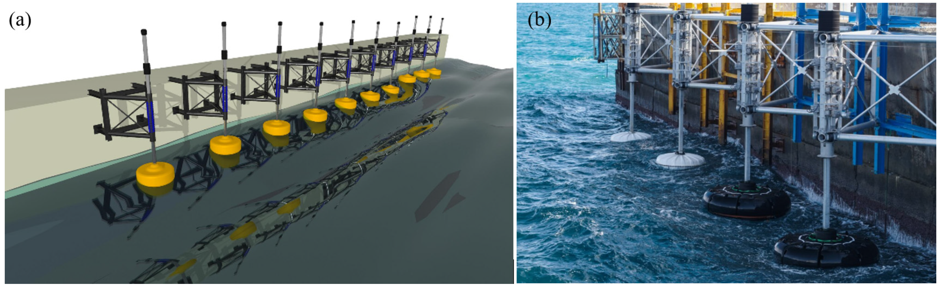
6]. The possibility of installing WEC arrays on the exposed side of breakwaters or piers was a subject of research in the past few years; see
Figure 1. Apart from obvious benefits regarding the facilitation of installation and maintenance, this can also augment the captured wave energy, due to effects of wall reflections that increase the responses; see, e.g., [
7,
8]. Recently, such deployments were tested in areas of increased wave potential, as in the case of the breakwater in the port of Heraklion in the northern-central part of Crete Island by SINN Power (
https://www.sinnpower.com, accessed on 29 July 2023), as shown in
Figure 1b. In such cases, the evaluation of long-term performance is supported by using high-quality, many years-long time series of wave data; see also [
9]. In addition, WEC-type absorbers integrated into floating breakwaters were both numerically and experimentally studied by Cheng et al. [
10], and the effects of various parameters and wave non-linearity are discussed. Additionally, integrated systems of breakwater WECs with other renewable energy converters for applications in the marine environment were recently studied and improvements of the combined performance are reported; see, e.g., [
11,
12].
Moreover, existing studies show that, for the hydrodynamic problems of multiple floating bodies, the so-called “gap resonance” phenomenon occurs in the narrow gap between the floating bodies when they are placed in close proximity [
13]. The occurrence of gap resonance could be helpful for improving the wave energy conversion efficiency of WECs. It was shown that when the gap resonance phenomenon occurs, the influence of fluid viscosity becomes significant, particularly for the heave motion of the floating structures [
14,
15], and should be considered; see also [
16,
17]. Although the classical potential flow theory does not consider the influence of fluid viscosity, which could lead to significant deviations at specific frequencies, it still provides useful results in an extended frequency band, which could be exploited for the evaluation of the system performance based on spectral average characteristics of the array response.
In this work, a 3D hydrodynamic model based on the boundary element method (3D BEM) is presented and discussed, aiming to evaluate the performance of WEC arrays consisting of multiple heaving bodies attached to the exposed side of a port breakwater. The latter is modelled as a vertical wall, taking into consideration reflective effects by the breakwater as well as hydrodynamic interactions between the multiple floating devices. Specifically, reflection effects are included in the BEM solver, assuming the deployment of a device at the exposed side of a breakwater. Numerical results of the predictions of power performance for various configurations are derived and discussed, including interactions of multiple WECs with the nearshore topography and the breakwater wall, as well as the effects of power take off (PTO) parameters. An important contribution of the present work is the development and testing of a first-order model that could provide, with relatively low cost, useful data for the preliminary design of complex WEC arrangements on breakwaters, over an extended incident wave frequency direction band, considering the long-term wave climatology of the installation site. The results could essentially support the selection of basic parameters including the PTO system and the preliminary evaluation of capital expenditures and operating expenses. As a demonstrative example, a case study is presented for a selected coastal site at the port of Heraklion, located in the north-central part of Crete Island in the South Aegean Sea, characterized by relatively increased wave energy potential in the region. Using long-term climatological data, the present method is illustrated and its applicability as a supporting tool for optimal design purposes is discussed.
The present work investigates the 3D hydrodynamic problem of several interacting heaving WECs, forming an array attached to a breakwater, based on linear wave theory. The method can be extended to investigate more general shapes of axisymmetric floaters in one or more degrees of freedom, as well as to study the effects of various control strategies, such as latching techniques to maximize the power output of the devices, by constraining some of the operational characteristics. The structure of the present paper is as follows: In
Section 2 the mathematical formulation of diffraction and radiation problems, involving multiple interactions of floating bodies operating as WEC point absorbers in front of a vertical wall, is presented, and the developed 3D boundary element method is discussed. Verification of the present model is included in
Section 3, along with discussion concerning numerical convergence. Systematic results for selected configurations are presented in
Section 4, also including the performance index of various members of the array. In
Section 5, the long-term performance analysis in the case of a particular site is examined using long-term climatological data. Annual and seasonal statistics of the power output prediction by the system are presented and discussed. Finally, in the last section (
Section 6), conclusive remarks are provided and directions for future research are discussed.
2. Mathematical Formulation and 3D BEM
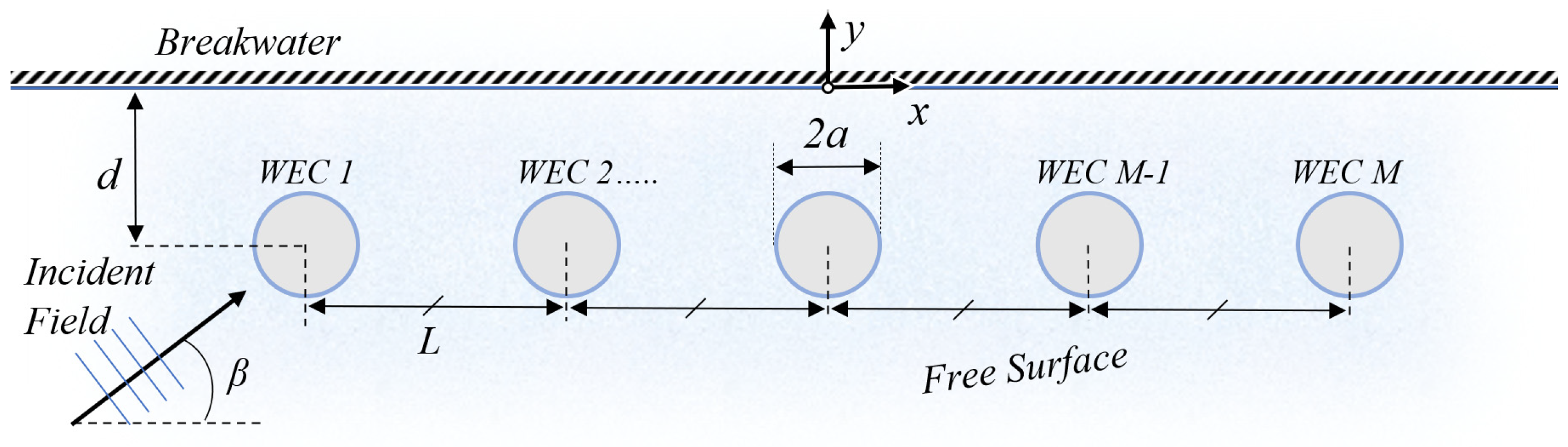
We consider an array of (single DoF) heaving point absorber WECs, consisting of
M identical devices, attached to the exposed side of a breakwater, and operating in constant local depth
h as shown in
Figure 2. The devices are subjected to harmonic wave excitation. The magnitude and phase of each WEC’s heave oscillation is derived by the analysis of the surrounding flow field in the domain
D, taking into account the hydrodynamic interactions among the WECs, as well as reflection effects due to the breakwater; see
Figure 3. Based on standard floating body hydrodynamic theory, the total field is decomposed into the incident, the diffracted and
M radiated subfields. The velocity field of each of the above is represented by the gradient of the corresponding potential function
, and
.
The coordinate system
is used, with the origin placed at mean water level (MWL) at the position of the vertical wall so that the center of each WEC’s waterplane area is located on the line
, parallel to the breakwater. The origin is selected so that the whole configuration is symmetric with respect to the
-plane, as schematically shown in
Figure 2 and
Figure 3. In this work’s context, cylindrical-shaped WECs of radius
and draft
are considered. However, the methodology presented can easily be extended to any device geometry. Results concerning the effect of different WEC shapes will be investigated in future works.
The above interaction problem is treated in the frequency domain, assuming harmonic time dependence in the form
, with
ω being the angular frequency and
the imaginary unit, by the representation:
where
A is the incident wave amplitude,
g is the acceleration due to gravity,
denotes the complex amplitude of the
mth WEC’s oscillation in the z-direction, and
is the complex potential in the frequency domain, which is given by:
In Equation (2),
and
stand for the complex amplitudes of the incident and the diffracted subfields, respectively, and
denote the complex amplitudes of
, evaluated for
. The complex potential of the incident field, incorporating the reflection effects due to the presence of the vertical wall, is assumed to be known, and for unit wave amplitude
is given by:
where
In the above equations,
β is the propagation direction (also shown in
Figure 2) and
R is the reflection coefficient, which eliminates the reflection of the incident field (
R = 0) in case of propagation parallel to the wall (
or
) or generates the reflected field (
R = 1) otherwise. Furthermore,
k stands for the wavenumber, obtained by the dispersion relation, as formulated in the local depth
h:
It is noted that Equation (3) presupposes a fully reflective vertical boundary of infinite length. The limitations of this assumption are investigated in Ref. [
7], where it is shown that it leads to reduced accuracy as regards the estimation of the heave excitation forces, especially at low frequencies, compared to more realistic, finite-length breakwater cases.
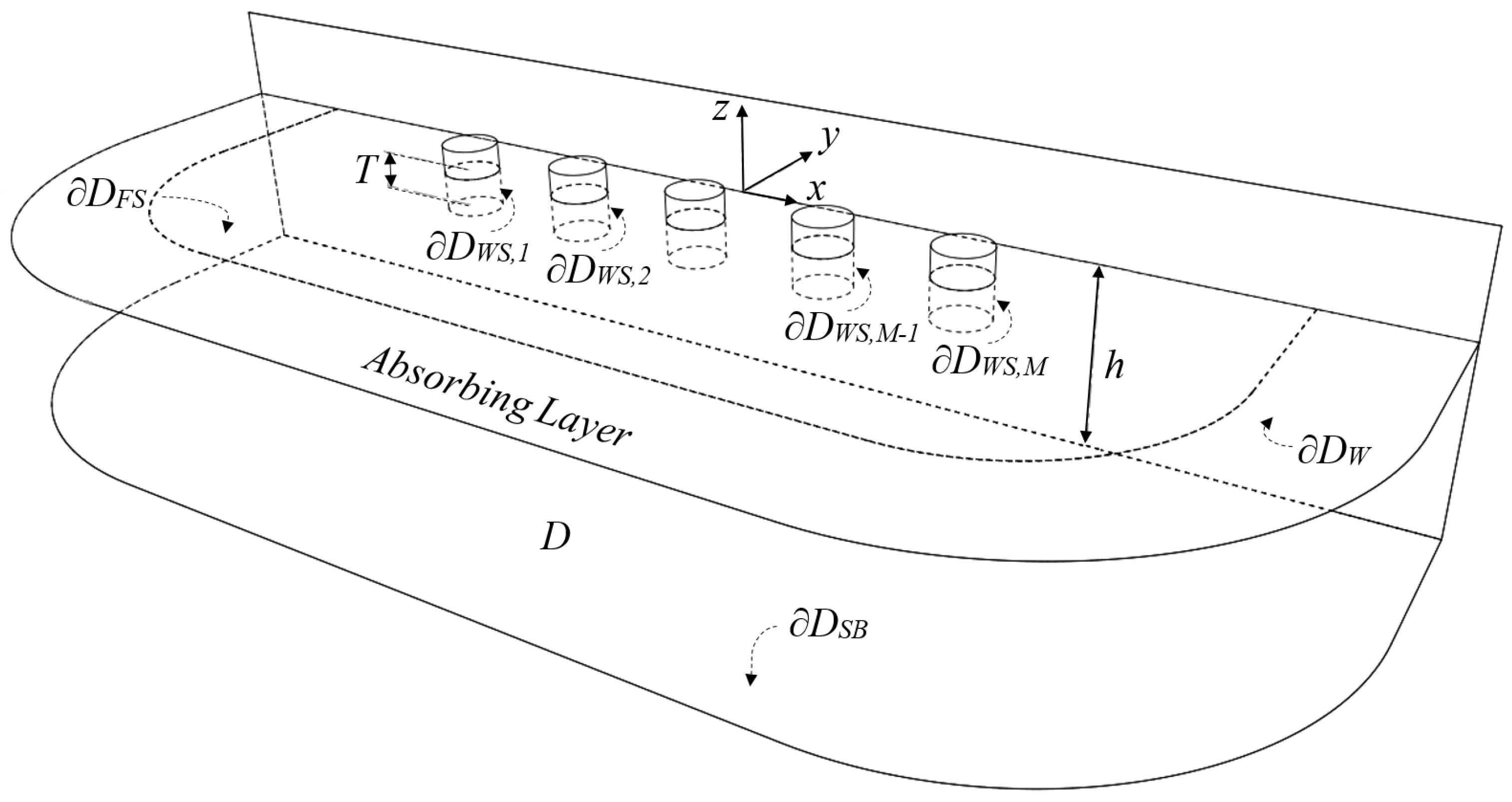
The diffraction and the
M radiation subfields are evaluated by boundary value problems (BVPs), governed by the Laplace equation, and supplemented by appropriate boundary conditions (BCs) at the various parts of the boundary
of the flow domain. The latter consists of the free surface of the water (
), the wetted surfaces of the WECs (
,
m = 1,2,…,
M), the impermeable boundaries of the wall (
), and the seabed (
); see also
Figure 3. Impermeability BCs apply to the solid boundaries, while the linearized free surface boundary condition (FSBC) applies to
. Therefore, the diffracted and radiated fields are evaluated as solutions to the following BVPs:
where
n = (
n1,
n2,
n3) is the unit vector normal to
, directed toward the exterior of the flow domain, and
in Equation (5d) is the Kronecker delta. The latter equation translates to the fact that the evaluation of the
m-th radiation field is achieved by enforcing unit excitation of the
m-th wetted surface, while treating the rest of the WECs as immobile and impermeable. Moreover,
is the frequency parameter, which is expressed as a function of space in Equation (5b) to account for modifications analyzed hereafter. The wave solutions calculated by the above BVPs propagate undisturbed towards infinity, which suggests that the flow domain extents infinitely to all azimuthal directions
. Therefore, numerical treatment requires the above problems to be supplemented by appropriate conditions at infinity. Truncation of the flow domain is achieved by adopting a perfectly matched layer (PML) technique (see
Figure 3), consisting of an absorbing layer, which is used to attenuate outgoing wave solutions and treat the radiating behaviour of the calculated fields at far distances from the WEC array, as described in detail in Ref. [
2]. The damping of outgoing waves with minimal reflection depends on the thickness of the layer, which is taken to be of the order of one wavelength
, while its coefficient is taken to be increasing within the layer. Implementation of the PML technique is achieved by making the frequency parameter complex within the layer to approximate artificial weakening of the wave solutions. Specifically, the frequency parameter is redefined as follows:
where
denotes the PML activation radius in the direction
The PML is activated on a curve defined on the MWL plane, as shown in
Figure 3. The parameter
c and the exponent
n are used as optimized in previous works [
2], aiming to the maximization of the layer’s efficiency, preventing numerical reflections, and avoiding contamination of the evaluated fields.
The BVPs described by Equation (5) are treated by means of a low-order panel method, based on simple singularity distributions and 4-node quadrilateral boundary elements, ensuring continuity of the geometry of the various parts of the boundary [
2]. The complex potential functions
, are represented by:
In Equation (7),
∂ denotes the boundary of
D, excluding the seabed part (
), while the homogeneous Neumann BC on the latter part is accounted for by using the following Green’s function for the Laplace equation in 3D in Equation (7):
which involves the contribution by the mirror point
with respect to the horizontal seabed plane
. Furthermore,
are singularity strength distributions defined on the boundary
∂, which are obtained by means of the low-order panel method, under the assumption of being piecewise constant on each element. The above distributions, in conjunction with a discretized form of Equation (7), reproduce the fields
. Specifically, the potential functions and the corresponding velocity fields are approximated by:
where the summation ranges over all panels, indexed by
p,
, is the singularity distribution’s strength on the
p-th element, while
and
, respectively, denote induced potential and velocity from the
p-th element (carrying unit singularity distribution), to the field point
x; for more details see [
18].
The numerical solutions are obtained using a collocation technique, satisfying each BC at the centroid of the corresponding panels on the different parts of the boundary (i.e., wetted surfaces, free surface, and wall). The impermeability BC on
is universally satisfied due to contributions by the mirrored points, while the computational boundary mesh does not need to include
, significantly reducing the computational cost. Using constant normal dipole distributions on each quadrilateral element, the induced potential matrix is analytically calculated via the solid angle; see [
19]. Moreover, exploiting the equivalence of a constant dipole element to a vortex ring, the calculation of induced velocity is obtained by repetitive use of the Biot–Savart law [
18]. As concerns discretization, a minimum of 15–20 elements per wavelength is applied to the discretization of the free surface boundary to eliminate numerical errors due to the damping and dispersion associated with the above numerical scheme.
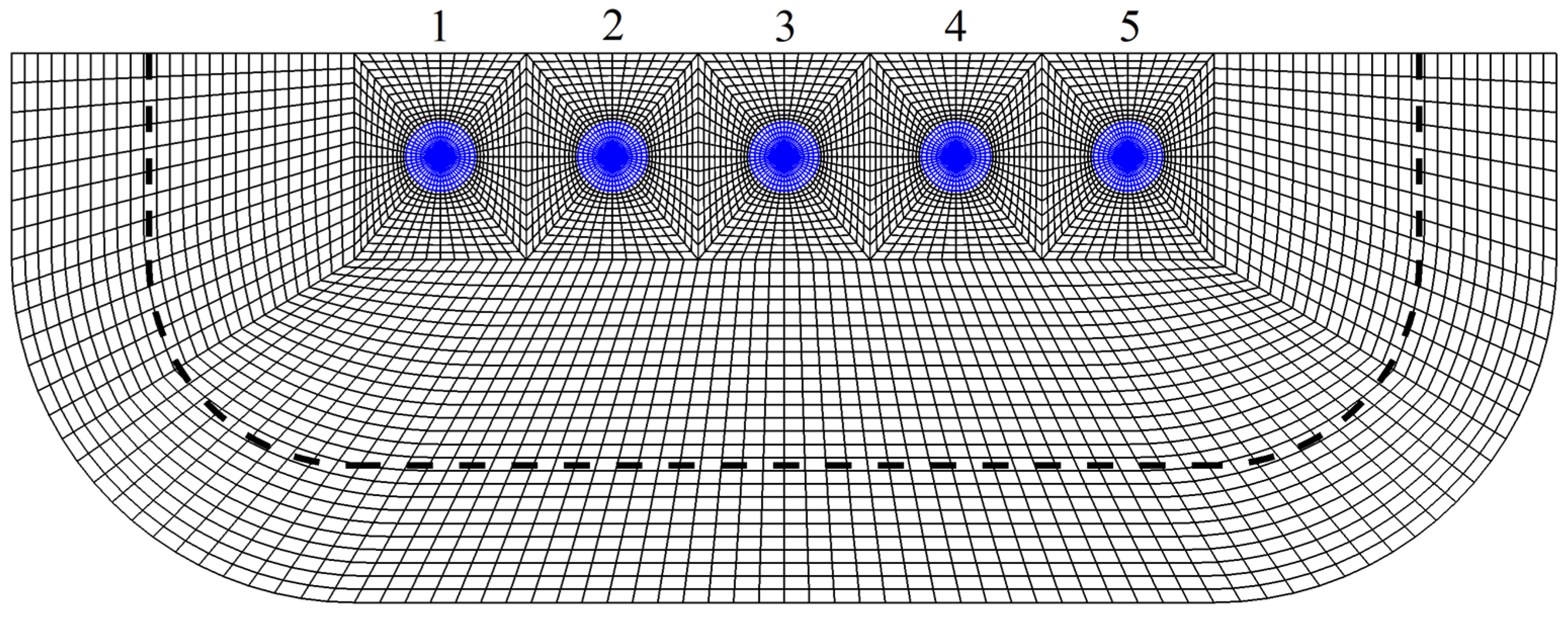
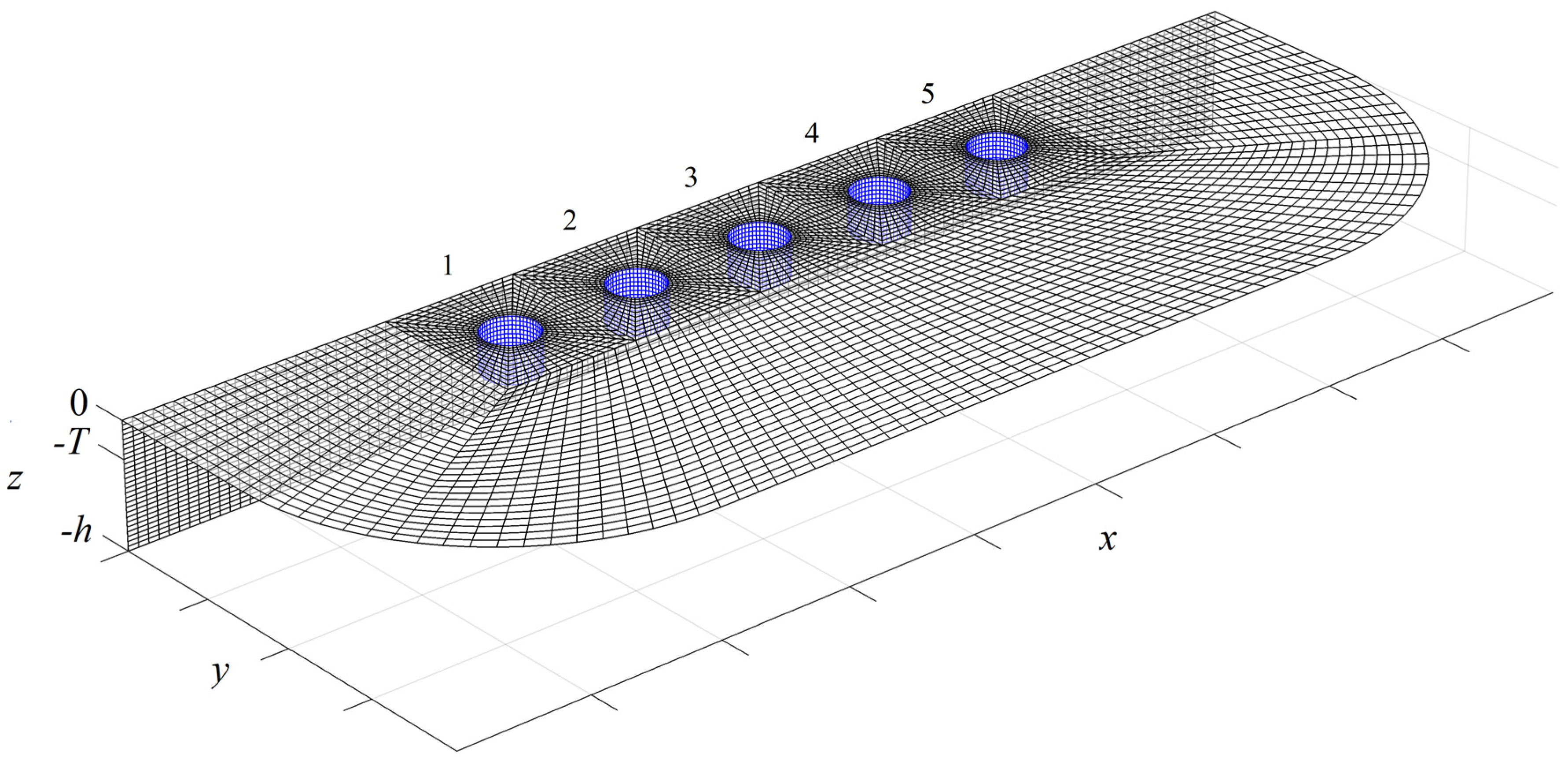
An important aspect of the BEM formulation is the mesh generation. The discretization is accomplished by incorporating corresponding structured meshes on the various boundary surfaces. Other important features are the continuous junctions between the different parts of the mesh, which, in conjunction with the quadrilateral elements, ensure global continuity of the boundary. An indicative boundary mesh of the flow domain consisting of 12,332 quadrilateral elements and containing 5 cylindrical WECs is presented in
Figure 4 and
Figure 5. As shown in these figures, sections of the free surface mesh are defined around each WEC to achieve continuity of the discretization. The surrounding free surface mesh spans a certain number of wavelengths and incorporates the absorbing layer. Furthermore, increased grid resolution is applied to the near field and on the wetted surfaces of the WECs for obtaining better quality results.
Having calculated the diffracted and radiated subfields, the heave response
of each WEC in the array is obtained by the following
linear system:
In Equation (10), the inertia of the WECs is modelled by the diagonal matrix
M = MI, with
, where
ρ is the water density. Furthermore, the effect of the hydrostatic restoring forces is modelled by the diagonal matrix
, where
is the identity matrix, and
is the heave hydrostatic coefficient, with
being the WEC radius. In addition,
models the extraction of energy from the power take off system, which is achieved by an additional damping coefficient, and
is the PTO stiffness. The elements of the added mass and hydrodynamic damping matrices
and
, respectively, are obtained via the calculated radiation fields as:
Moreover, the Froude–Krylov and the diffraction excitation forces on the
m-th WEC are calculated by integration of the pressure induced by each of the fields multiplied by the vertical component of the normal vector
n:
The mean output power of the each WEC device is then evaluated as:
where
stands for the efficiency of the electromechanical PTO system, and thus the performance index is defined by normalizing the above result with respect to the incident wave power flux over the cross section of the device, given by the WEC waterline diameter, considering a wave of height
H = 2
A:
where
denotes the wave group velocity.
3. Model Verification
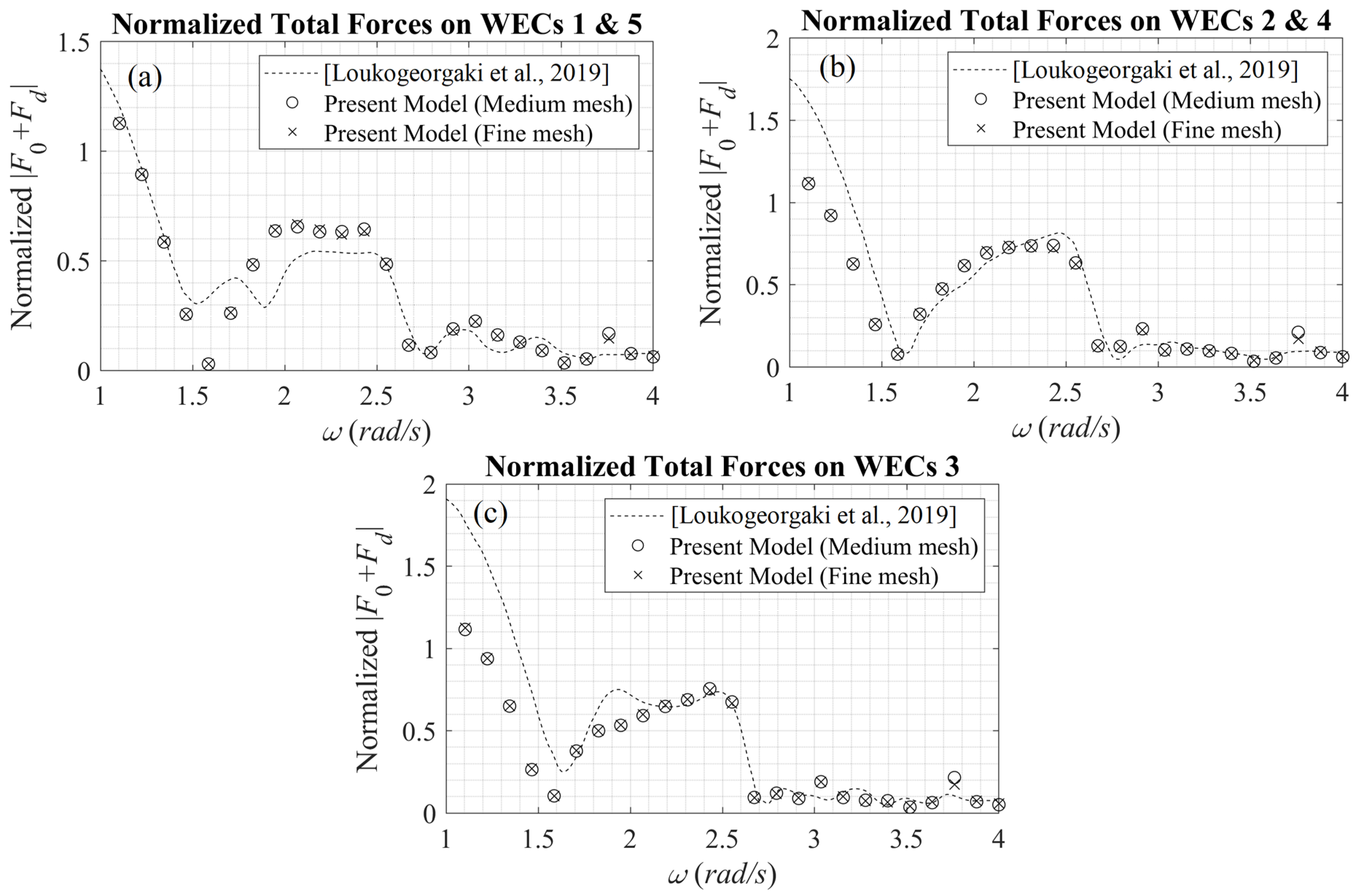
In this section, results obtained by the present model are compared against data from previous research for verification. The total Froude–Krylov (FK) and diffraction vertical forces exerted on five cylindrical WECs of an array operating in a region of water depth
h = 10 m in front of a vertical impermeable wall are examined; see
Figure 5. The propagation direction is
β = 90°, corresponding to normal wave incidence to the wall, and thus, both the incident and diffracted fields present symmetry with respect to the central body. Therefore, the total forces acting on the devices 1 and 5, as well as the ones acting on devices 2 and 4, are the same. The WECs’ diameter is
and the draft is
. The distance from the wall to WEC central axis is
and the non-dimensional distance between two adjacent WECs is
. The above configuration was recently studied by Loukegeorgaki et al. [
8] in the case of finite breakwater length.
Figure 6 depicts the present method results concerning the normalized total forces
F/
ρgAπα2, exerted on each WEC of the array, as functions of the angular frequency
ω, in the range [1 rad/s, 4 rad/s], as calculated by the present model. The results are derived from the present BEM based on two different computational grids with different numbers of elements in order to verify the convergence of the results. In particular, a medium and a fine mesh are used. In the medium mesh, the wetted surface of each cylindrical WEC is approximated by 1044 quadrilateral elements, while in the fine mesh configuration, each WEC is represented by 1584 elements. The surrounding free surface mesh spans 2.5 wavelengths and is redefined for each frequency. The latter boundary part incorporates the absorbing layer, which is activated one wavelength before the edge of the grid. In the medium mesh case, the free surface is discretized by 15 elements per wavelength and the total mesh size varies from 22,000 to 26,000 elements (for higher frequencies). The increase in the number of elements is a consequence of maintaining a minimum of 15 elements per wavelength on the free surface parts surrounding the WECs, and increased grid resolution is used in the near field; see
Figure 4 and
Figure 5. In the finer mesh case, the free surface is discretized by using 17 elements per wavelength and the total mesh size varies from 32,500 to 38,600 elements. As observed in
Figure 6, the medium mesh provides convergent results for all frequencies.
Moreover, in
Figure 6, comparisons of the present BEM predictions with the results of Ref. [
8] are shown by using dashed lines. As remarked above, in the latter work, the breakwater wall length is finite and equal to
, and thus, the WEC array extends over the whole breakwater. On the contrary, in the present model, the far-field radiation condition is implemented by using an absorbing layer technique, and the results practically correspond to infinite breakwater wall length. The above remark justifies the differences observed between the two data sets. For angular frequencies lower than 1 rad/s, due to the substantial increase in the wavelength, the consideration of the finite breakwater wall configuration of Ref. [
8] results in reduced reflection effects as compared to the present method, which is responsible for the differences concerning the excitation forces, and therefore, also the responses, especially in the low frequency band. On the other hand, the infinite wall assumption of the present model results in full-wall reflection of the incident wave for all wavelengths, and the WEC responses that will be examined in more detail in the next section, especially for very low frequencies, are affected by the stationary field generated by the combination of the incident and reflected wave components.
4. Numerical Results
Numerical results are presented in this section for the case of an array consisting of five cylindrical WECs installed in an area of water depth
with
,
,
. In the absence of data concerning values of
, numerical results for
are obtained and presented. Moreover, representative values for
are used, where
denotes a characteristic value obtained as the frequency average of the calculated hydrodynamic damping coefficient
, corresponding to the middle (third) WEC of the array, and
j is a multiplying factor, defined as
. The PTO stiffness is taken to be
, corresponding to magnitudes used in the literature; see e.g., [
20]. The case
is additionally considered, corresponding to an array consisting of freely floating bodies.
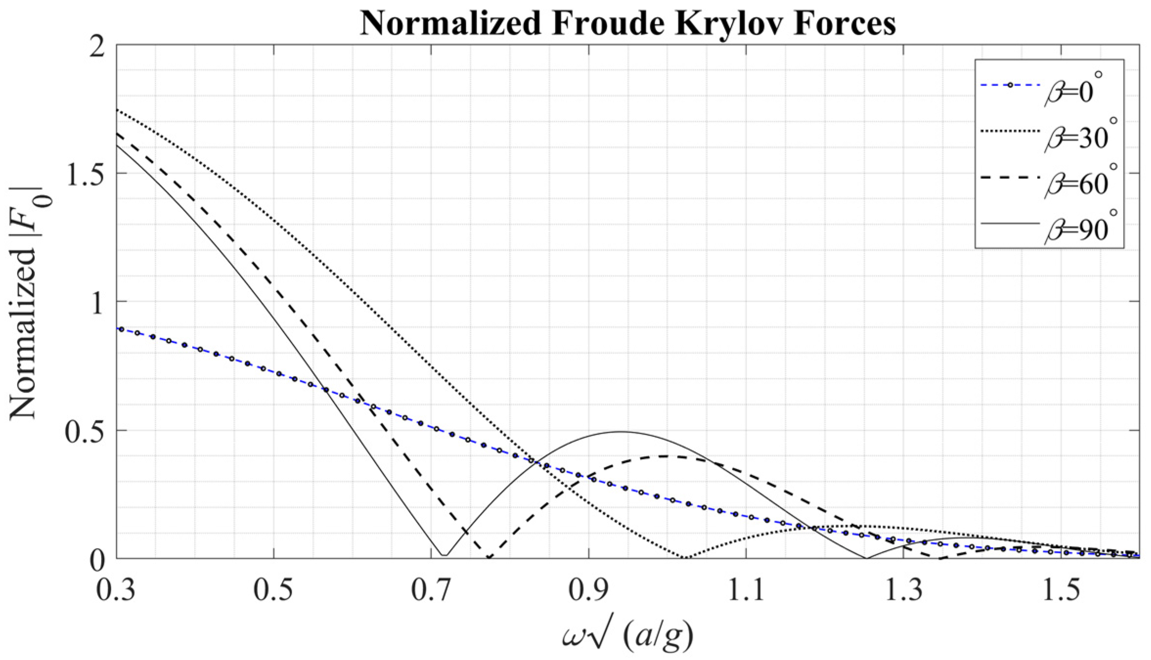
The Froude–Krylov (FK) vertical forces acting on the WECs, normalized with respect to (
ρgπAα2), are depicted in
Figure 7, as functions of the non-dimensional frequency
, showing a strong dependence on the direction of propagation of the incident field. In particular,
Figure 7 shows the FK forces resulting from propagation at incident wave directions
, and
, with the
case corresponding to normal incidence on the wall. The case
, corresponding to incident wave propagation parallel to the breakwater, is also included. The position of each device only affects the phase of the FK forces, except for the
case, where these forces on all WECs share the same phase. It is observed in
Figure 7 that in the low-frequency limit and
different than zero, the normalized FK forces tend to 2, which is due to wall reflection effects on the wave field, since all WECs are placed on an antinode. On the contrary, for
the wall reflection is zero and has no effect. However, the latter case is not expected in practice, since for breakwaters in nearshore/coastal regions, the bathymetry-induced refraction and shoaling effects on the wave propagation will result in incident waves with a direction component towards the wall.
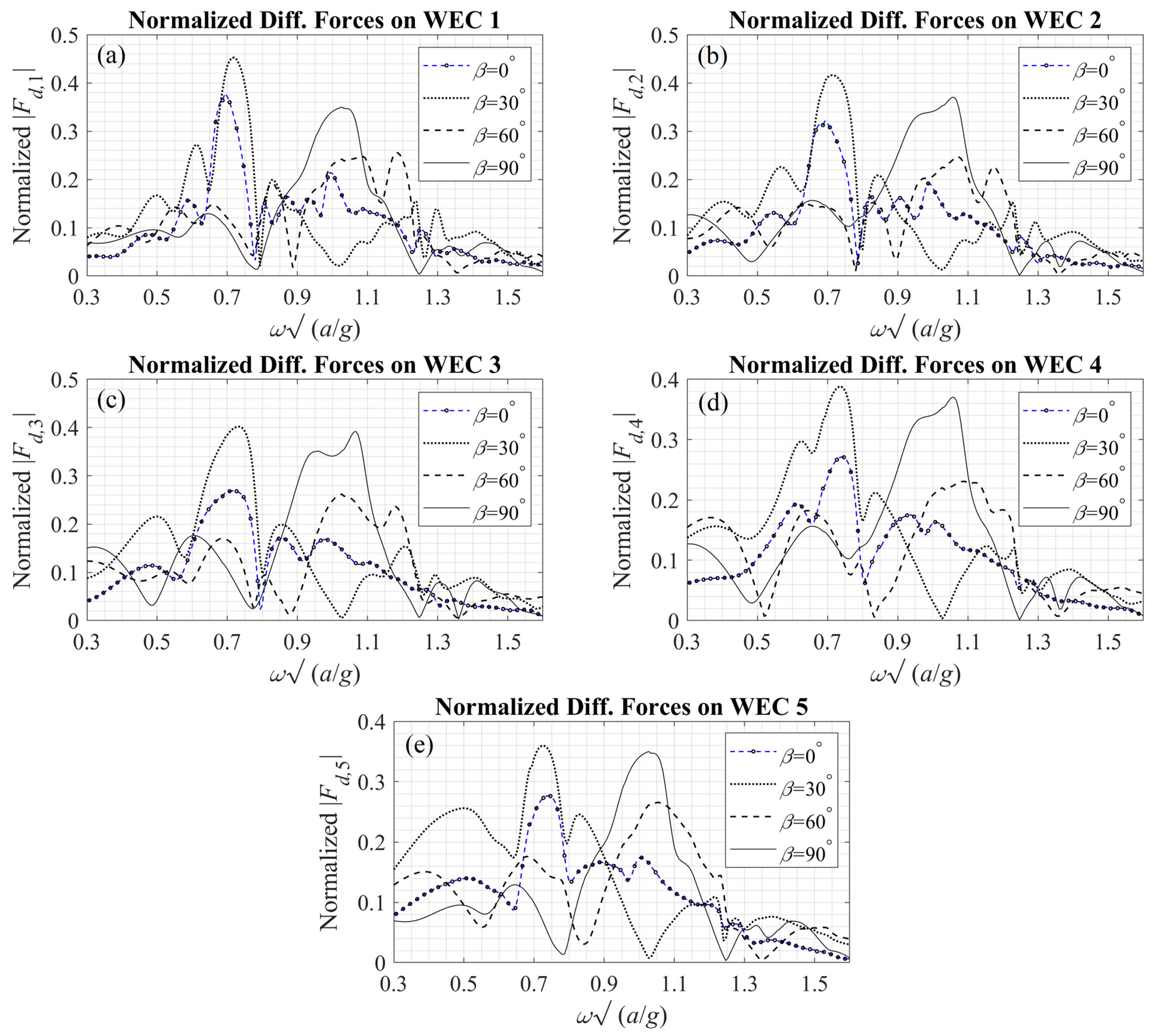
Moreover, the diffraction forces on each WEC are shown in
Figure 8, and it is observed that they present a complicated pattern as a result of the wall’s presence. Furthermore, the diffraction forces on the WECs 1 and 5, as well as on the WECs 2 and 4, are equal in the case of normal incidence to the wall (
) due to symmetry of the arrangement and the resulting fields. It is noted that the diffraction forces are different for each WEC in the arrangement, as opposed to the FK forces.
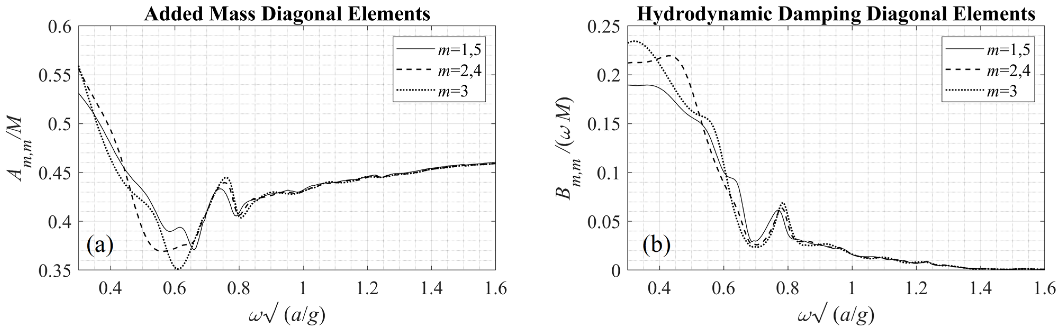
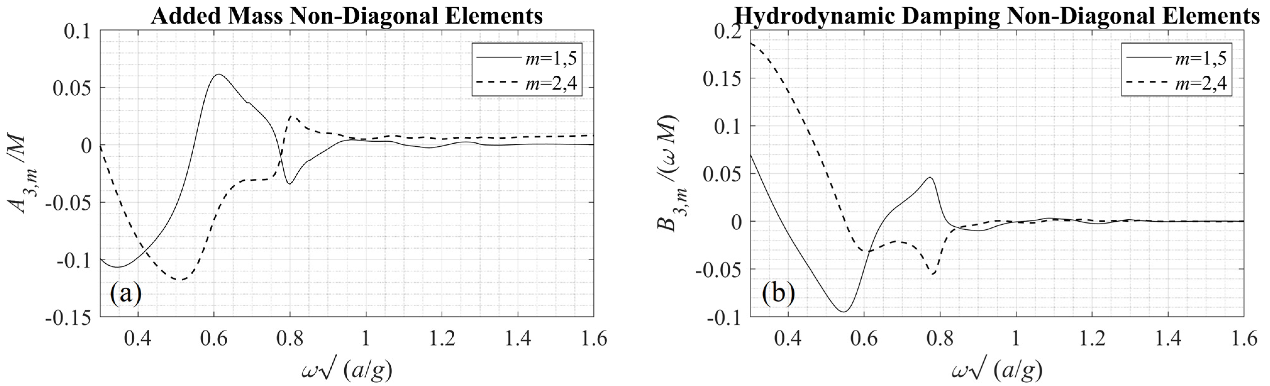
Data concerning the diagonal components of the added mass and the hydrodynamic damping matrices are presented in
Figure 9. In particular,
Figure 9a shows the diagonal elements of the added mass matrix
A (normalized with respect to the mass of each WEC:
) and
Figure 9b shows the (non-dimensional) diagonal elements of the hydrodynamic damping matrix
B as functions of the non-dimensional frequency
. For comparison, non-diagonal elements of the
A and
B matrices, corresponding to the middle (third) WEC of the array are presented in
Figure 10.
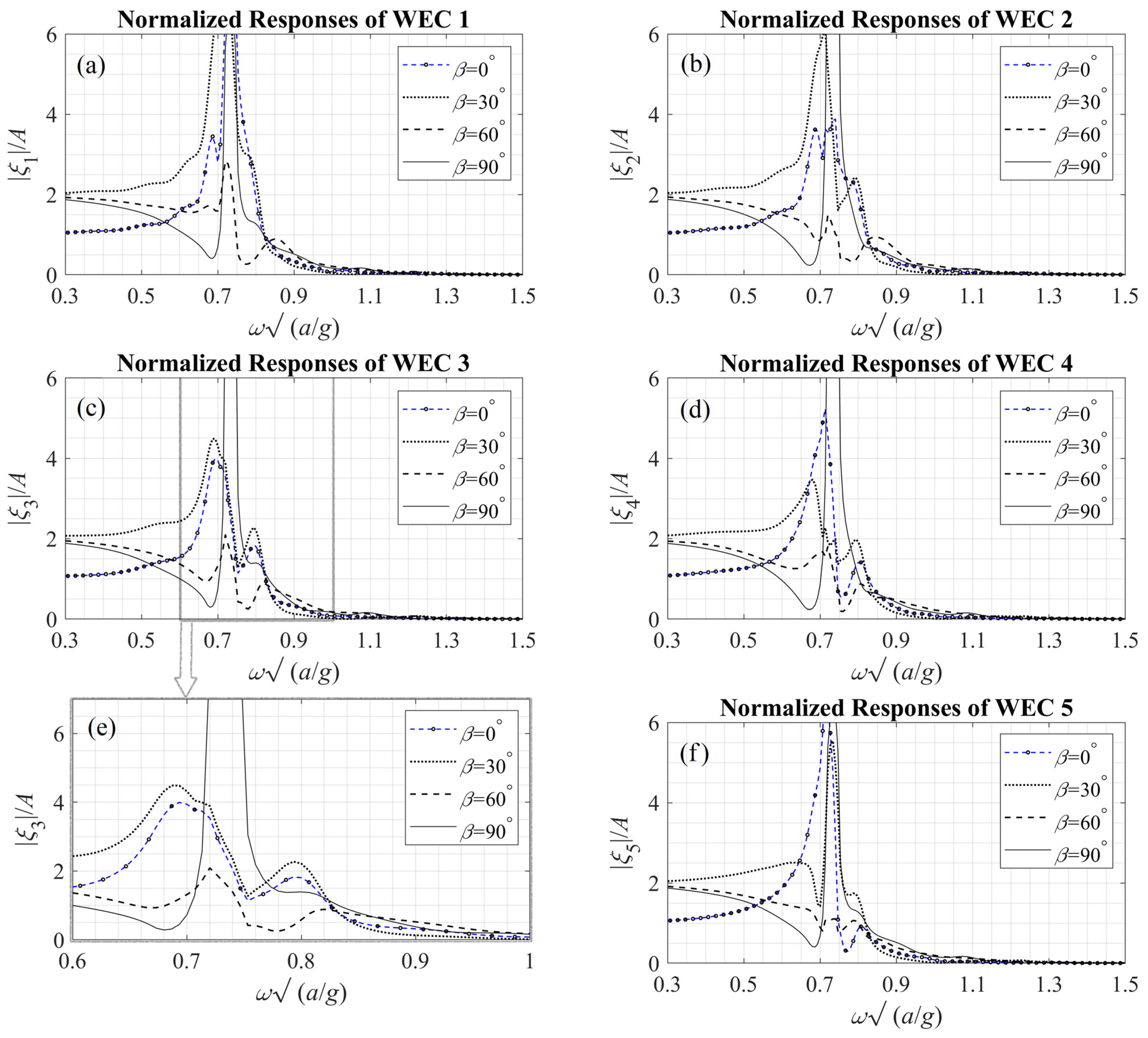
The response amplitude operators (RAOs) of each WEC are shown in
Figure 11 for
, as functions of the non-dimensional frequency
for the case of freely floating bodies (
). In this case, it is observed in
Figure 11 that the responses become significant for frequencies near the resonance, especially for
, as illustrated in subplot (
e) of
Figure 11, which shows a zoom-in of the response of the central WEC in the band of frequencies near resonance.
It is worth noting that the responses of the WECs are highly dependent on the gap between the devices and the vertical wall. Especially in the case of normal incidence, the formation of standing waves leads to low responses when the WECs are centered on a node of the incident field, which corresponds to wavelengths of
λ such that
, where
is the distance from the WEC waterplanes’ midpoints to the breakwater; see
Figure 2. For the considered case, this happens for wavelengths corresponding to non-dimensional frequencies
and the RAOs present a pattern similar to that of the FK forces, which vanish at these points, as shown in
Figure 7.
The effect of the PTO parameters on the devices’ responses is illustrated in
Figure 12 for
. In particular,
Figure 12a–c shows the responses of WECs 1 and 5,
Figure 12d–f shows the responses of the WECs 2 and 4, and
Figure 12g–i shows the responses of WEC 3 as functions of the non-dimensional frequency. The PTO stiffness (
) is set to
in the first column of
Figure 12, while in the subplots of the second and third columns, it is set to
and
, respectively. The various subplots of
Figure 12 illustrate the responses for
. The above, for a dimensional configuration with
, respectively, correspond to the following values of the damping coefficient:
,
,
, and
, respectively.
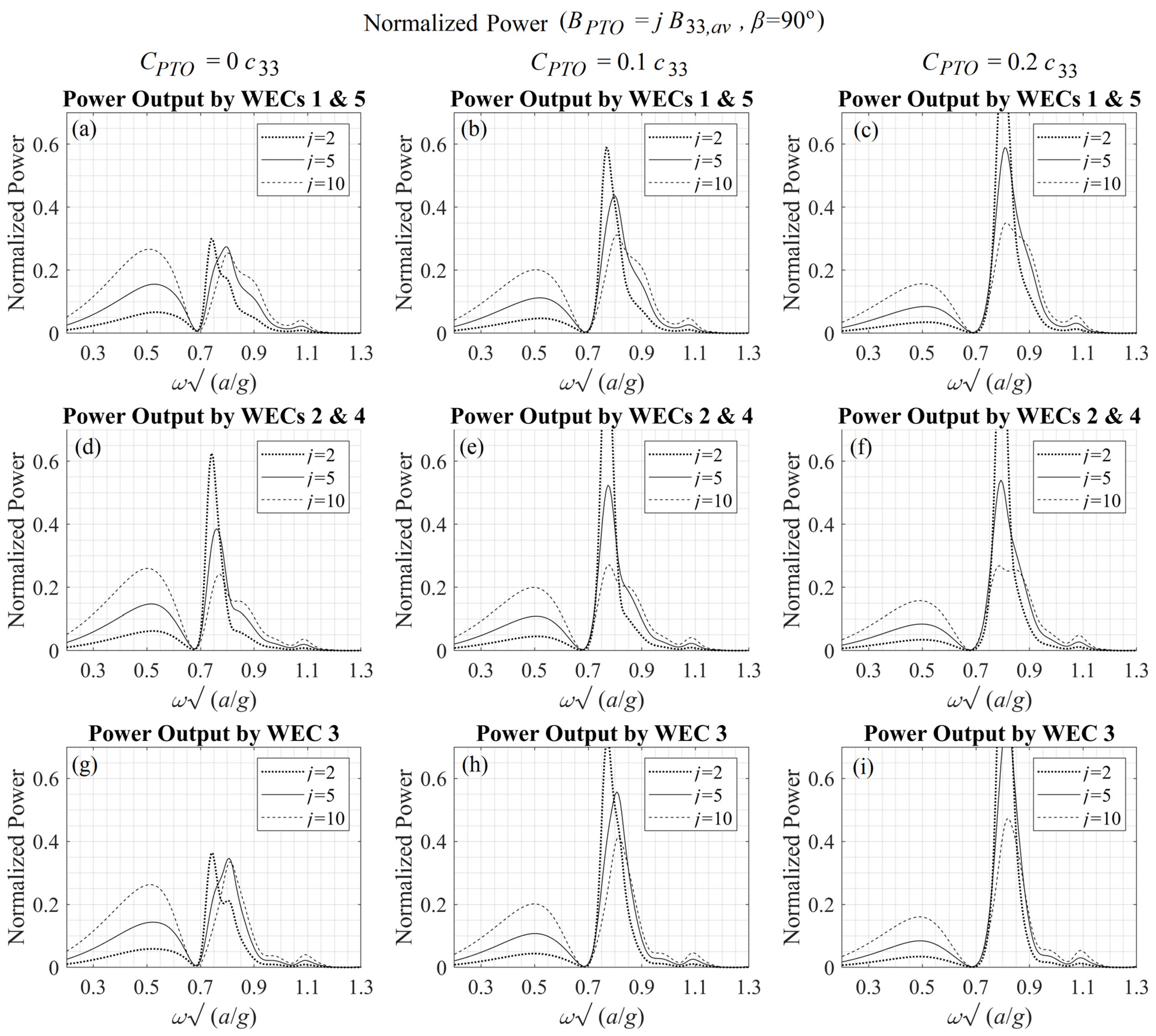
The resulting performance index (normalized power output) for each WEC of the array, as evaluated by Equation (14), is illustrated in
Figure 13. Specifically,
is shown in the first-row subplots (a, d, g),
in the second-row subplots (b, e, h), and
in the third-row subplots (c, f, i). As expected, higher values of PTO damping lead to decreased peak values of heave response. However, at the same time, they lead to increased power absorption at low frequencies, as shown in
Figure 13, since the power output of the WECs’ is directly related to the PTO damping, while the RAOs at frequencies below resonance are not gravely affected. As regards the PTO stiffness, it can be seen in
Figure 12 that higher values of
, slightly shift the natural frequency and tend to keep the responses lower at the low frequencies range.
The present analysis concerns the ideal flow case and serves as a first approximation for the estimation of the system performance. Effects of viscosity on the responses, as well as on the gap resonances could be approximated by introducing additional damping and this is left to be examined in future extensions of the present model.
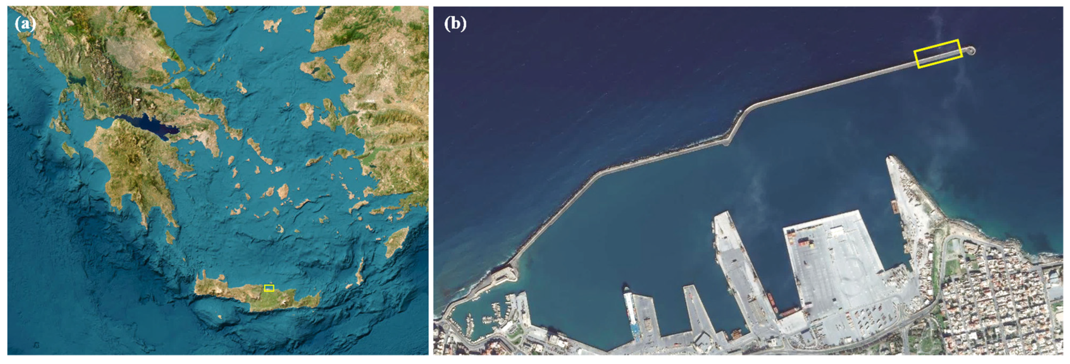
5. Case Study
The nearshore area at the port of Heraklion, situated in the north coast of Crete Island, in the Southern Aegean Sea, is studied as an example of the application of the considered system in the Greek seas region; see
Figure 14. The above nearshore area is characterized by relatively increased wave potential [
21] and is thus considered to demonstrate the applicability of the present method, as regards the evaluation of the WEC array’s power output.
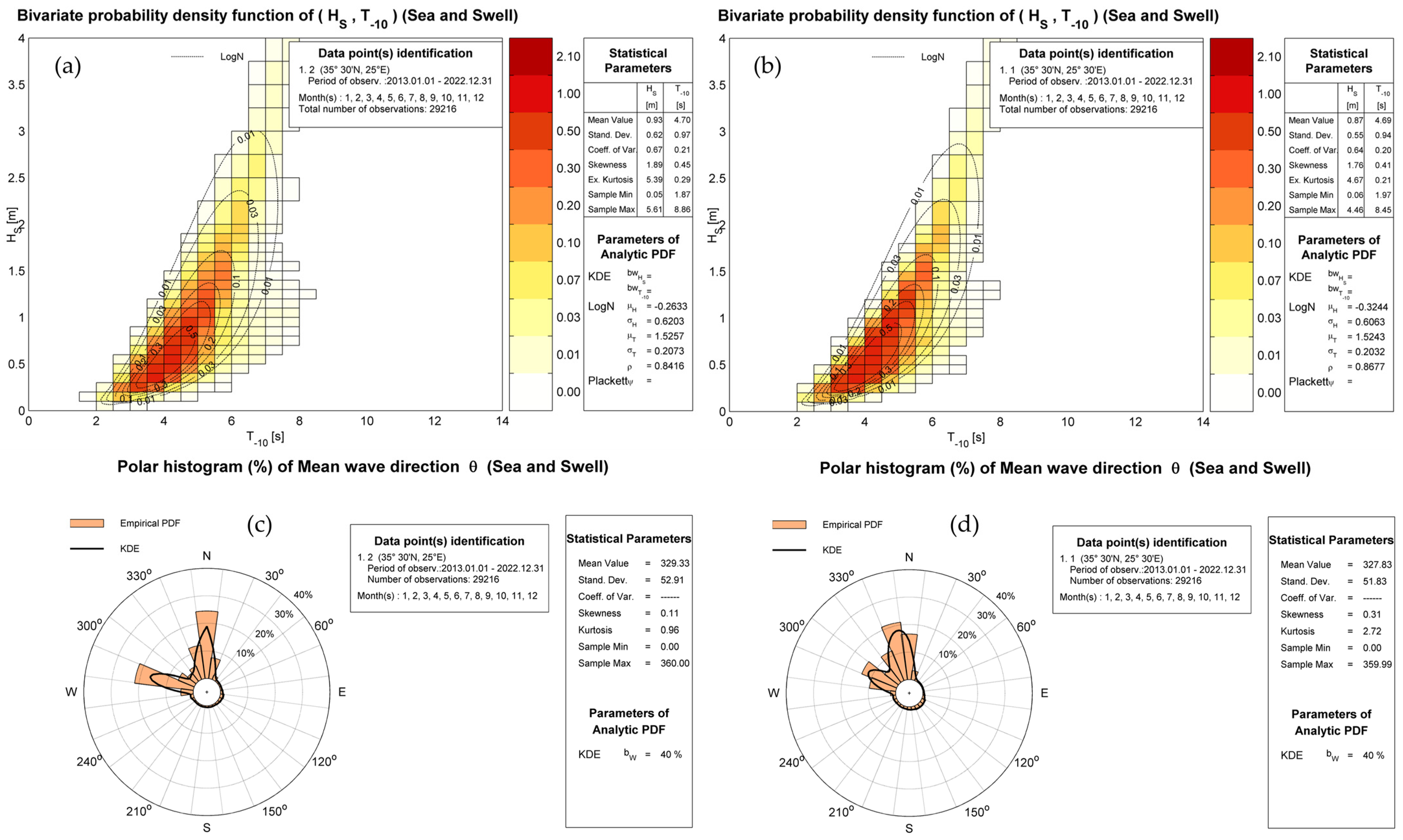
The wave climatology in the studied area is based on a long-term time series, covering the 10-year period between January 2013 and December 2022, at the offshore points with geographical coordinates 35°30′00″ N–25°00′00″ E and 35°30′00″ N–25°30′00″ E, as derived from the ERA5 database [
22]. The relevant information includes significant wave height (
HS), mean energy wave period (
T-10), and mean wave direction (
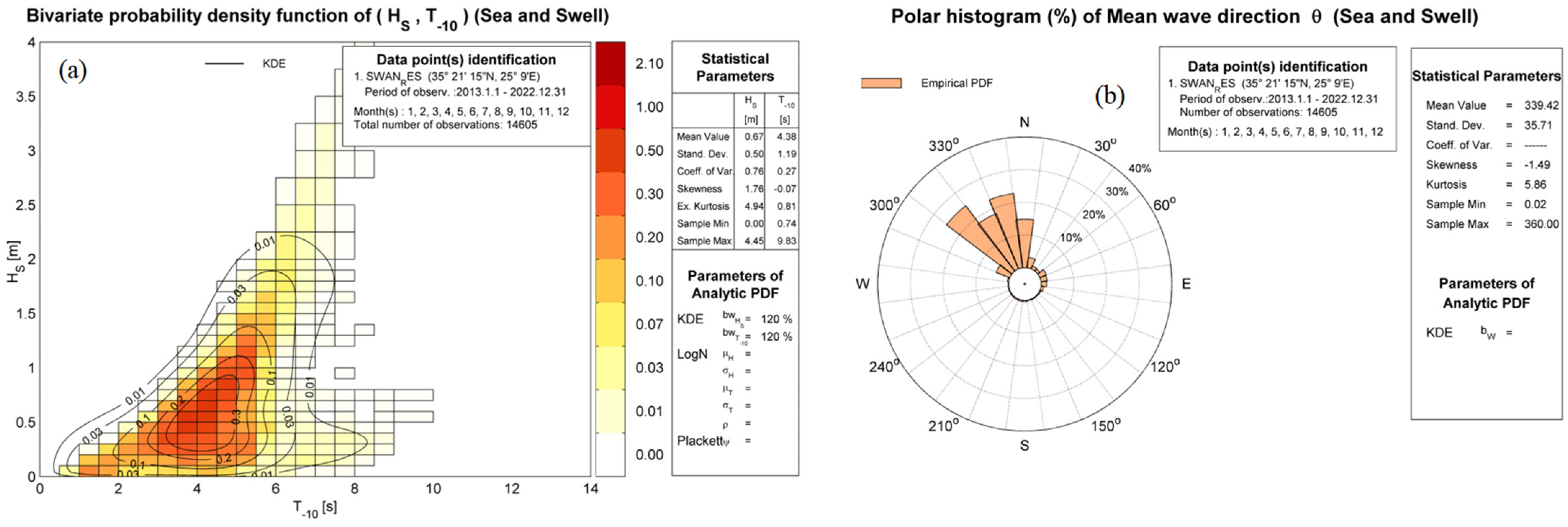
θm—measured clockwise from the North) with a 3 h temporal resolution. Based on the above data, the offshore wave climatology is derived and presented in
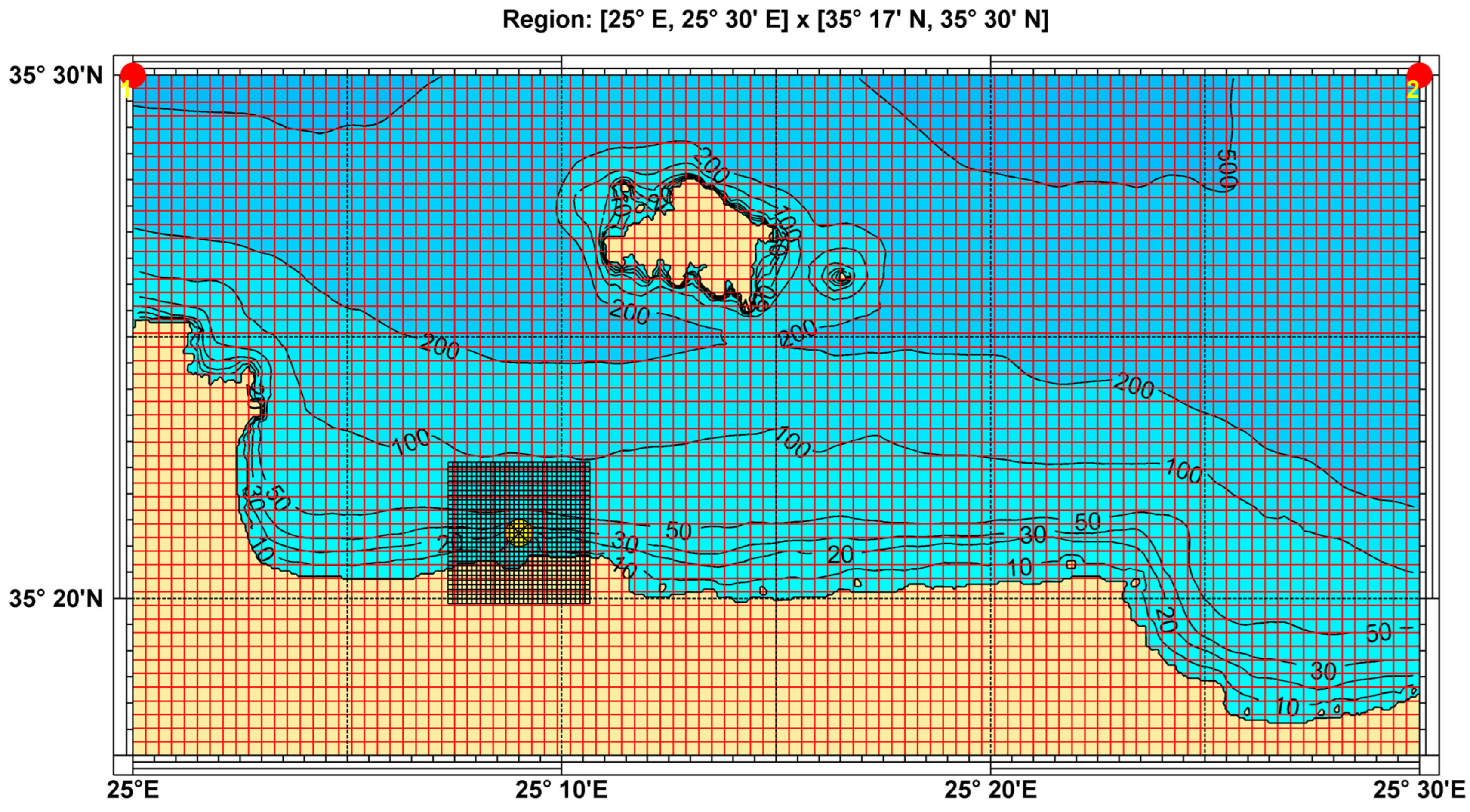
Figure 15, where standard lognormal and kernel density univariate and bivariate models are used to represent the distributions. An offshore-to-nearshore (OtN) transformation technique is used to generate nearshore wave data at the target point located at a distance in front of the breakwater with geographical coordinates 35°21′15″ N–25°09′00″ E, as shown in
Figure 16. Calculations are based on the SWAN nearshore wave spectral model [
23].
Offshore wave conditions, represented by appropriate spectral parameters (significant wave height, mean wave period, and mean wave direction), are considered known all along the seaward boundary from which directional spectrum
is reconstructed using the JONSWAP frequency spectrum, in conjunction with a hyperbolic cosine spreading function. For the present study, the bathymetric data used are obtained from the General Bathymetric Chart of the Oceans (GEBCO) [
24]. The database used for the coastline is the Global, Self-consistent, Hierarchical, High-resolution Shoreline Database (GMT—GSHHS), provided under GNU Lesser General Public License; see [
25]. The main forcing of the examined system is represented by the offshore wave conditions, which are continuously distributed along the seaward boundary. Given the offshore boundary conditions, the phase-averaged model SWAN is applied to calculate the wave conditions inside the computational domain with sufficient spatial resolution, as shown in
Figure 16. The basic equation used in SWAN model is the radiative transfer equation expressing action balance:
where
denotes the wave action density, expressed as a function of spectral density
and wave frequency
. Furthermore,
, and
denote propagation velocity components in the physical and the Fourier parameter space, respectively, and
models the forcing source terms, including the effects of wind-generated wave energy, dissipation due to deep-water wave breaking, wave–seabed interactions, and depth-induced wave breaking in shallow water. More details concerning the implementation of OtN wave transformation can be found in Ref. [
26].
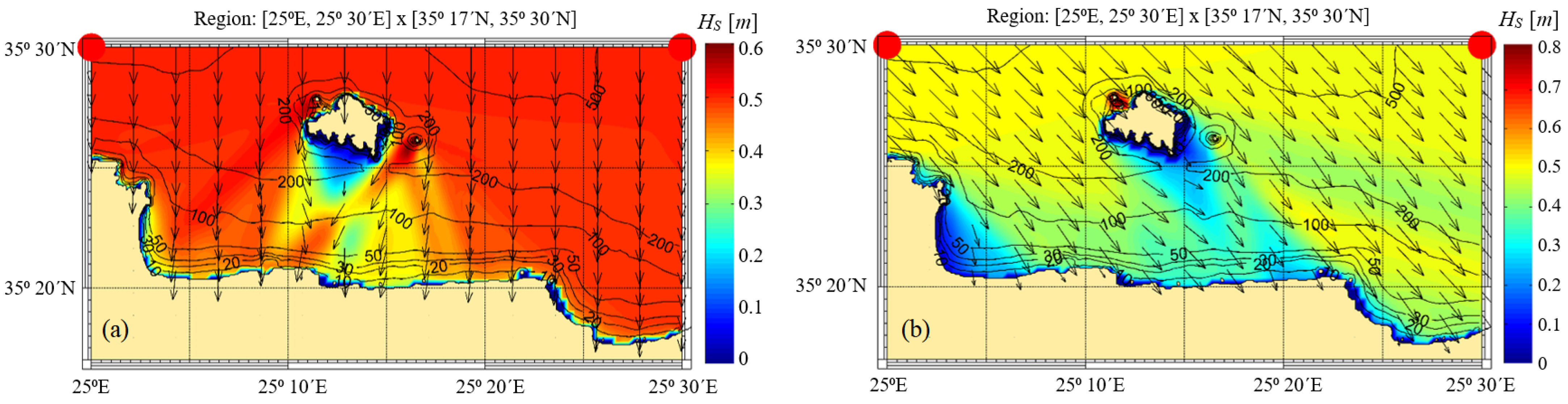
Selected results are presented in
Figure 17 concerning the spatial distributions of the calculated significant wave height in the domain corresponding to characteristic wave conditions at the offshore boundary. It is clearly seen in this figure that the transformation of wave conditions includes refraction–diffraction and shoaling effects, as well as the sheltering effects by the small island (Dia) at the northern side of the domain. The derived nearshore wave climatology, at the target point located at a distance about 3.5 km from the port of Heraklion breakwater and water depth
h = 15 m, as obtained by the present OtN transformation, is presented in
Figure 18, and the corresponding basic statistics of the nearshore wave parameters are listed in
Table 1.
In order to quantify the examined WEC array’s power output, we consider the five cylindrical WEC arrangements in Heraklion port breakwater where the local depth is equal to
. The floater radius is
and a PTO system is considered with
, which corresponds to
, and C
PTO = . Considering all incident wave energy concentrated in the normal direction of the breakwater, the 10-year-long time series of nearshore wave parameters is used to reconstruct wave spectra using the TMA model [
27]:
where
denotes the JONSWAP spectrum and
the TMA filter function; see also [
7]. Each reconstructed spectrum in the time series is discretized into a large number of frequencies
, where
denotes the corresponding constant spacing, and the output power time series of the 5-WEC system is estimated as follows:
where
and
denotes the normalized power output of the
k-WEC, at frequency
and the given
, that is estimated using data from
Figure 13.
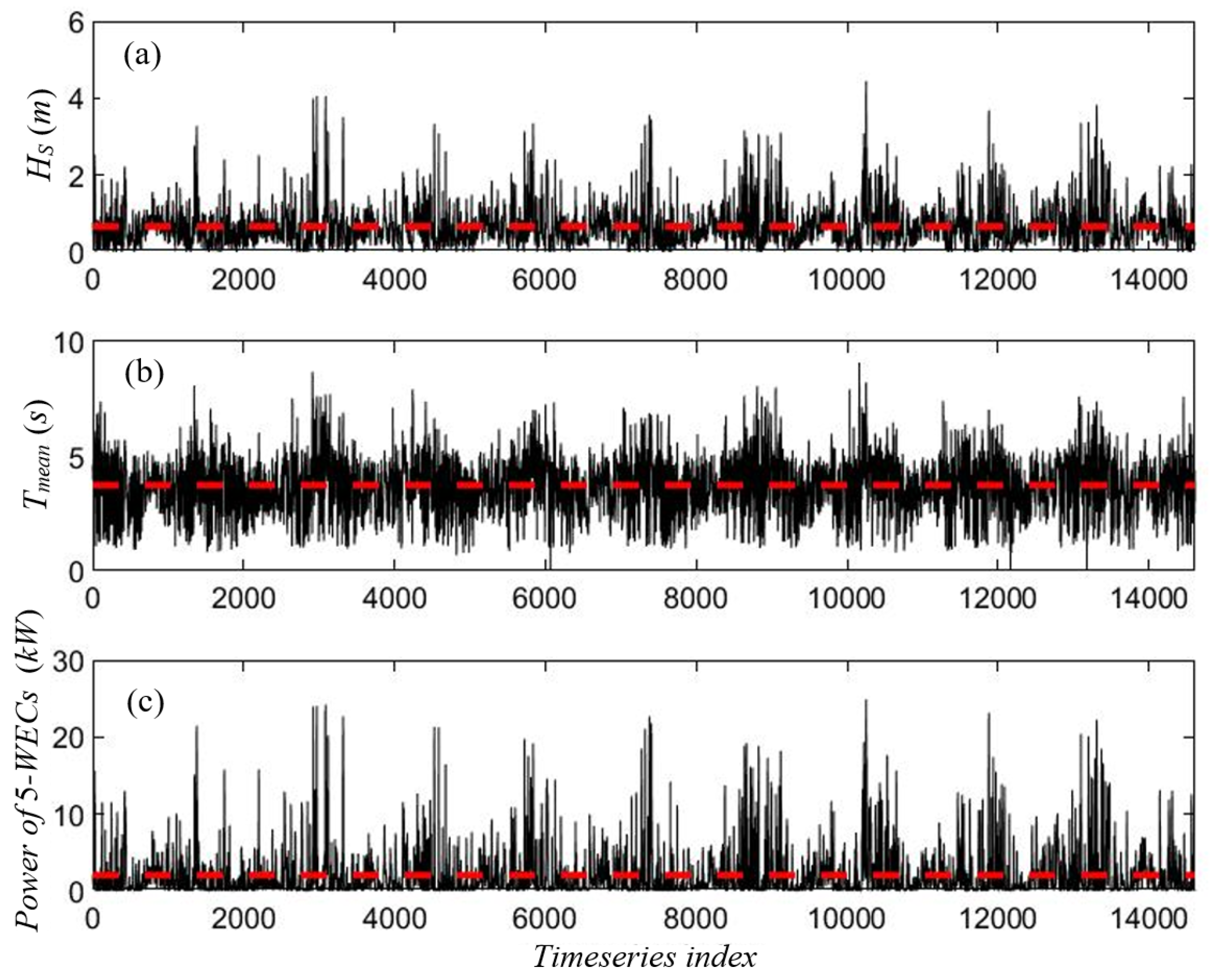
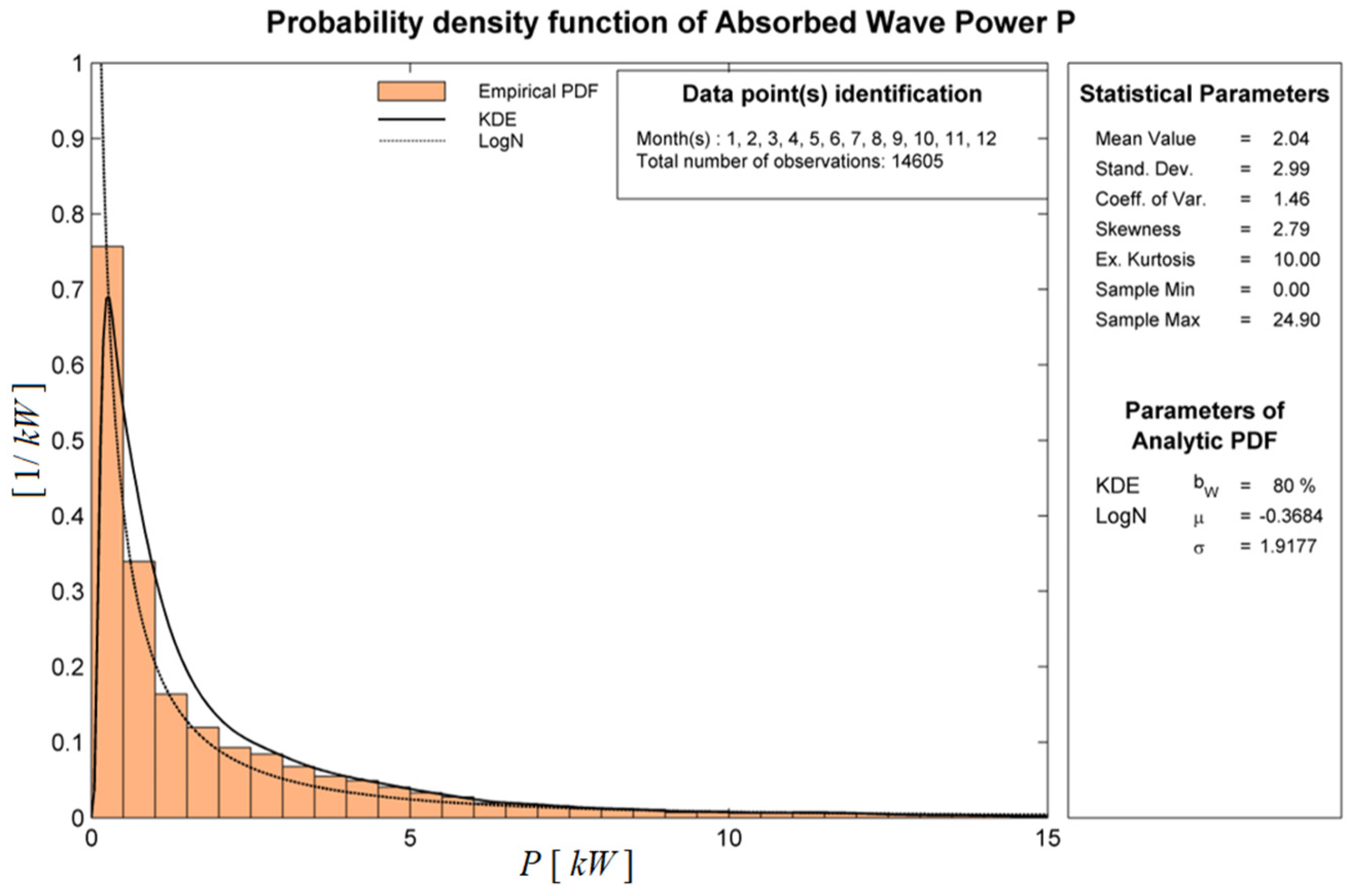
In
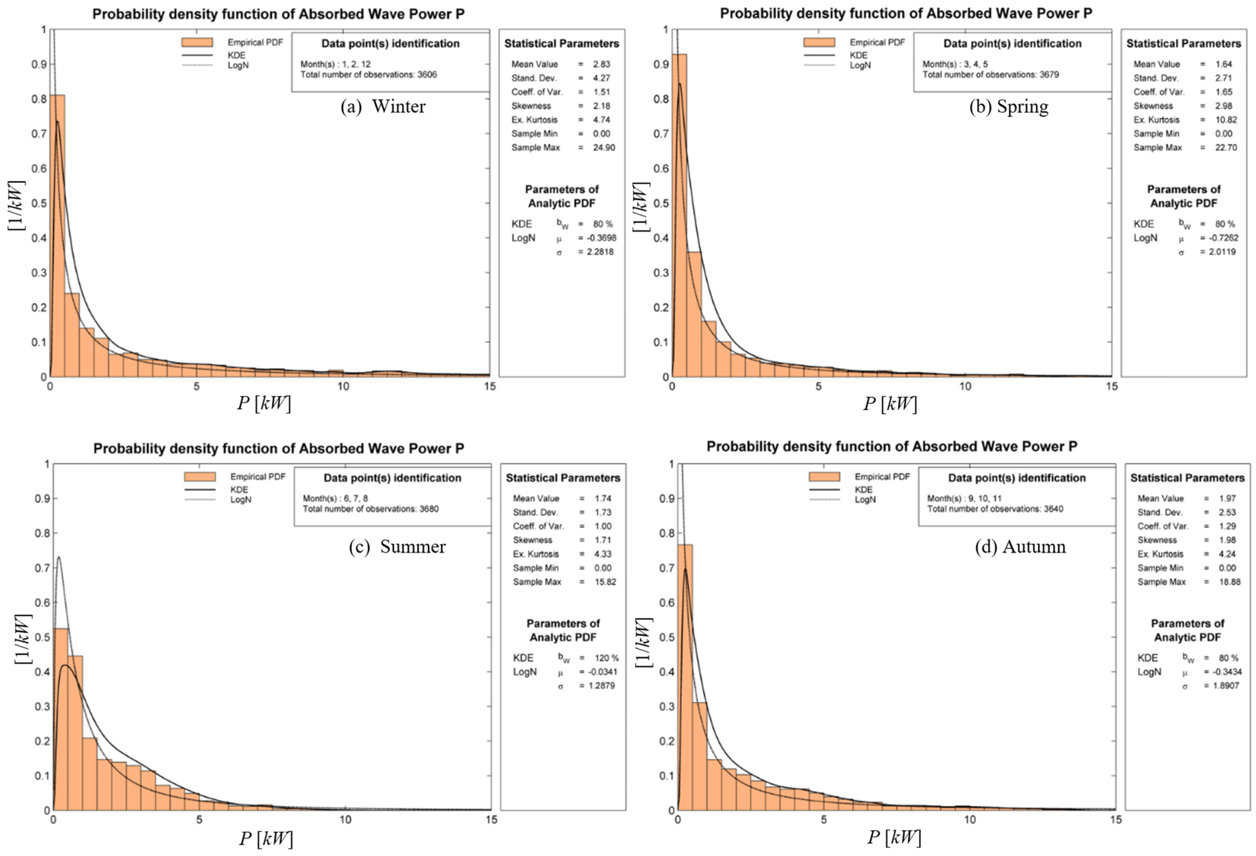
Figure 19, the calculated 10-year-long time series of nearshore wave data and power output, by the considered 5-WEC arrangement at the breakwater of Heraklion port, is shown. The annual and seasonal statistics of power production by the system is presented in
Figure 20 and
Figure 21, respectively, including data concerning mean values and important statistical parameters. Based on the above analysis, the mean power output by the system is 2.04 kW, corresponding to an annual energy production of 17.7 MWh, and the power production is ranging from zero to a maximum value of about 25 kW. For comparison, the corresponding output concerning the same system without the breakwater wall effect is estimated to be 2.3% lower. The energy production by the studied configuration could be further improved by optimal design, and the studied system considered together with the benefits from the facilitation of installation and maintenance of the system and the connection to the grid, could be important for the further consideration of these systems contributing to the greening of energy in ports and harbors.
Regarding practical applications of the considered energy stations, it is evident that the selected devices’ natural period in heave can be selected or tuned to coincide with the wave period carrying the highest amounts of energy based on local wave climatology in order to maximize the power production. Further improvement of power output can be achieved by systematic application of the developed BEM model to optimize geometrical, inertial and PTO parameters, and will be the subject of future works. Moreover, in order to reduce the computational cost, the BEM model could be used to derive reduced order models, as the one presented in Ref. [
6], which could substantially support the design of the system, by the fast scanning of the multidimensional parameter space, identifying subdomains of best performance. The 3D BEM could be used at the final stage for detailed detection and verification of the optimal solution.


