
Protection Scheme for Transient Impedance Dynamic-Time-Warping Distance of a Flexible DC Distribution System

Abstract
:1. Introduction
- (1)
- Given the extremely high action time requirements of DC distribution systems, the influence of line-distributed capacitance cannot be ignored. The protection scheme should have strong resistance to distributed capacitance currents.
- (2)
- The topology of distribution systems containing distributed power is complex and the selectivity of single-ended schemes is poor. The proposed scheme should compensate for this selectivity deficiency.
- (3)
- DC system faults develop very fast, and smaller communication delays may lead to the failure of the protection scheme. The proposed scheme should be acceptable for larger communication delays.
- (1)
- The fault characteristics of the transient impedance are analyzed, and the transient impedance is calculated using the traveling wave signal so that the proposed scheme is not affected by the distributed capacitance.
- (2)
- The normalized DTW distance of the transient impedance at the local end is calculated and judged, and only the judgment result is transmitted to the opposite end. This process allows the proposed scheme to accept longer communication delays.
- (3)
- Compared with the prior state of the art, the proposed solution ensures high resistance and noise interference capability with better quick action.
2. Expression Derivation of Transient Impedance
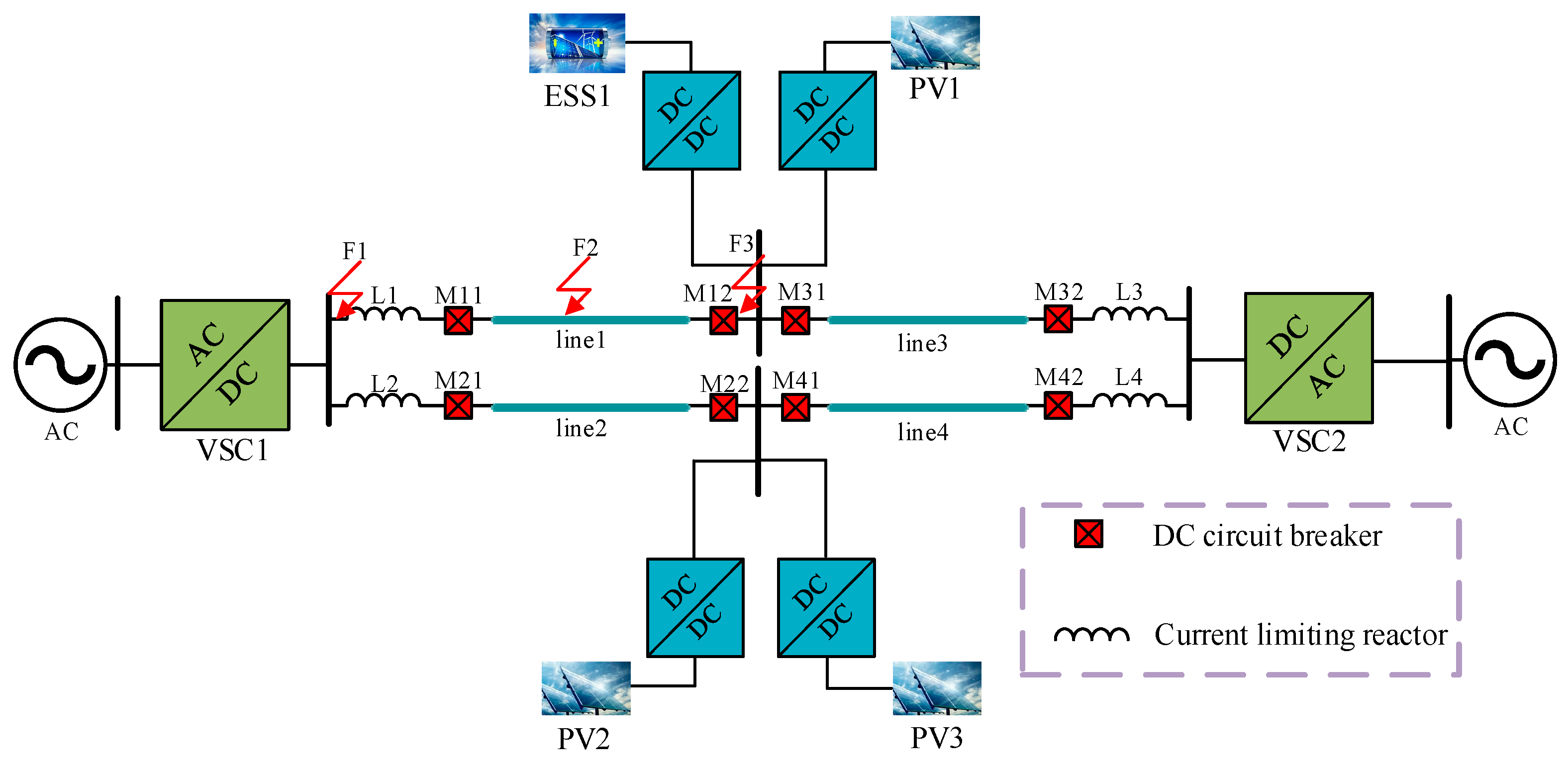
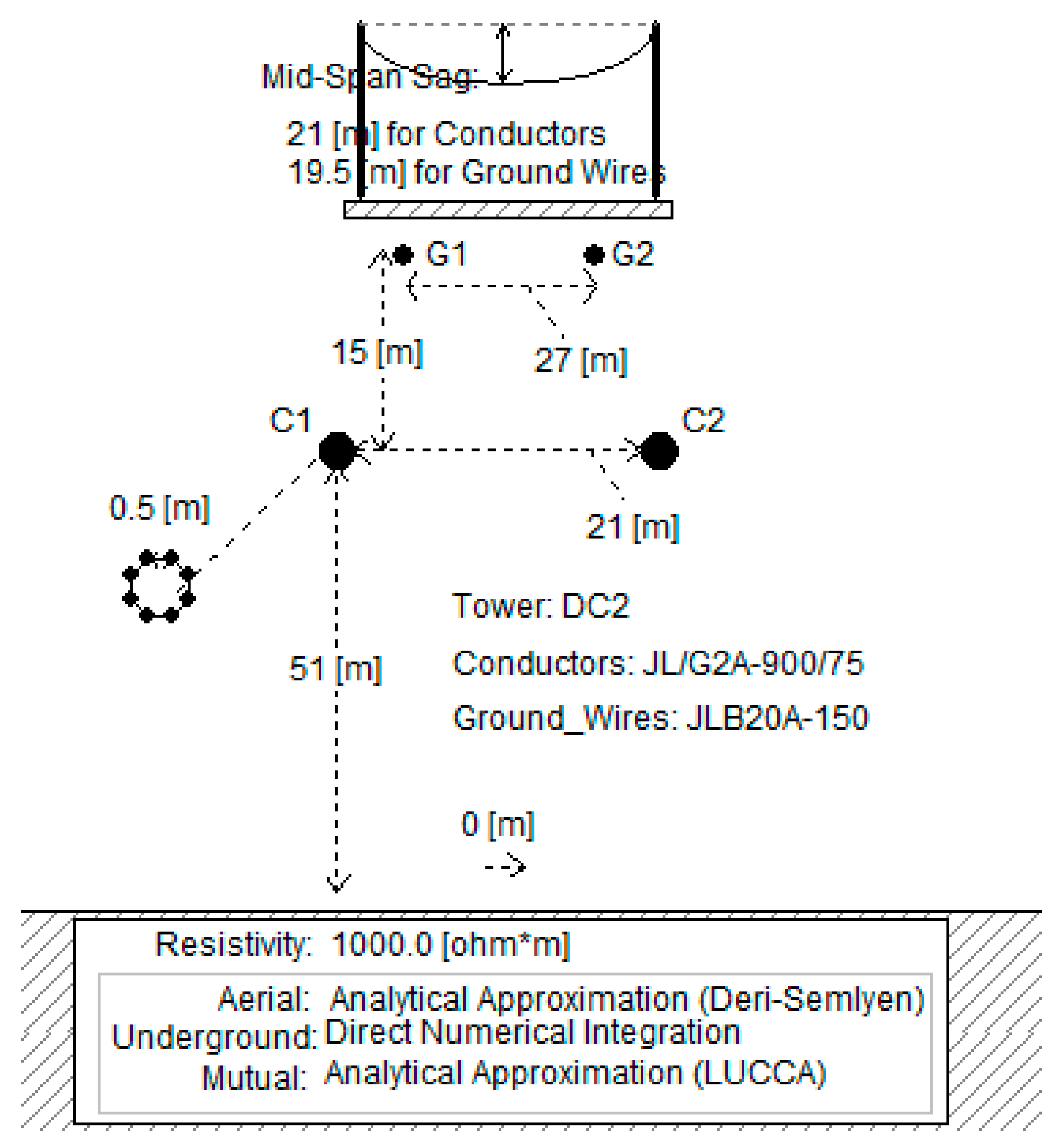
2.1. Models
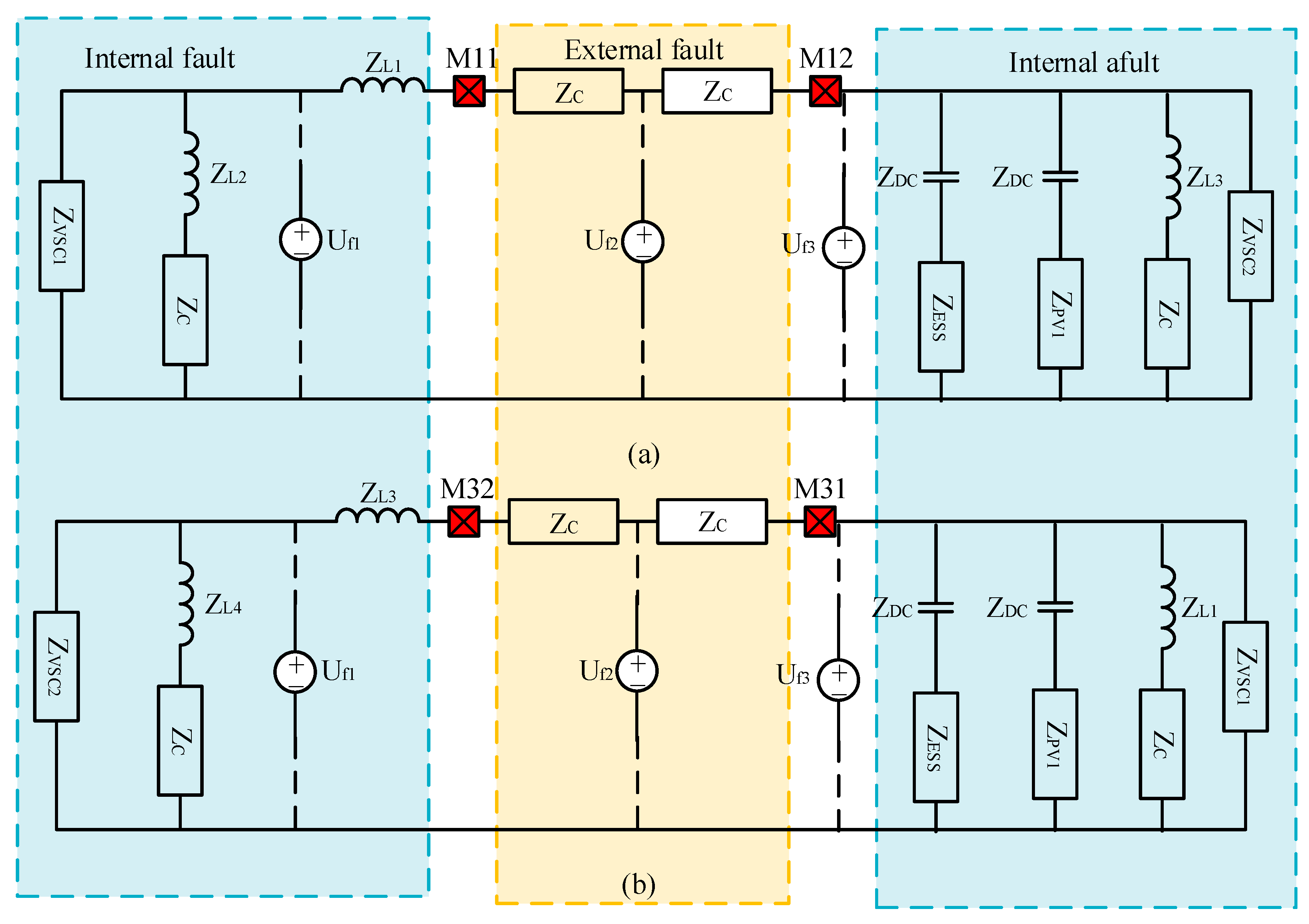
2.2. Equivalent Circuit of Line1 and Line3
- A.
- Line1
- B.
- Line3
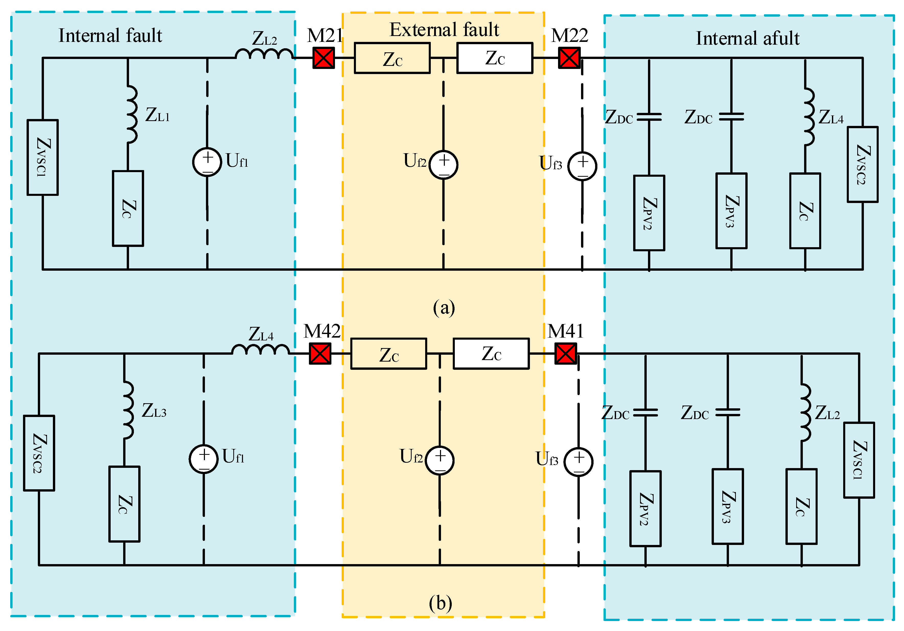
2.3. Equivalent Circuit of Line2 and Line4
3. Analysis of Transient Impedance Difference
3.1. Transient Impedance of Line
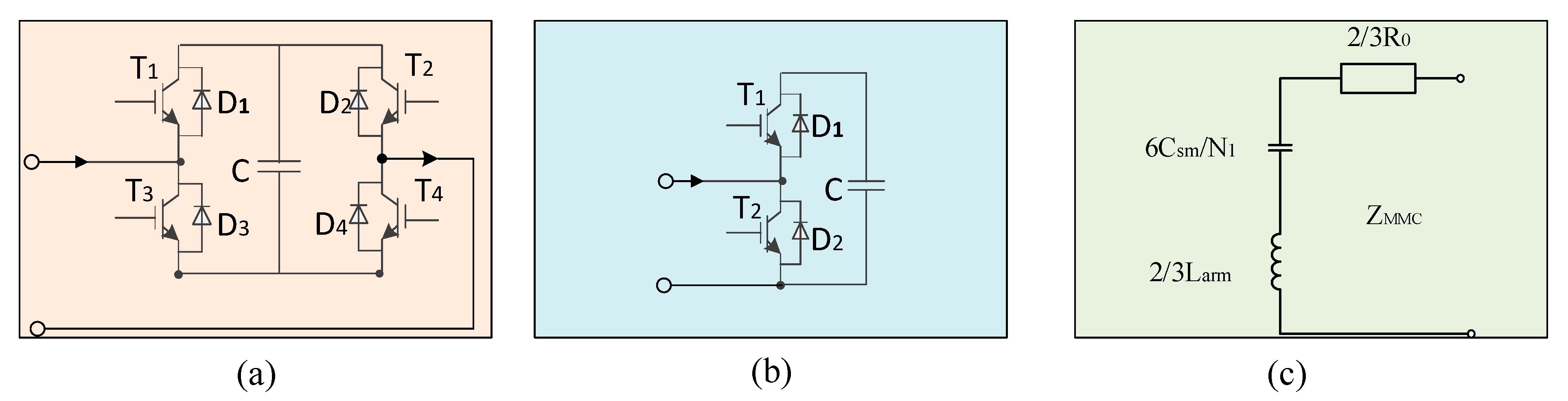
3.2. Transient Impedance of Voltage Source Converter
3.3. Transient Impedance of Current Limiting Reactor and DC/DC Converters
3.4. Transient Impedance of Photovoltaics
3.5. Transient Impedance of ESS
4. DTW-Based Protection Scheme
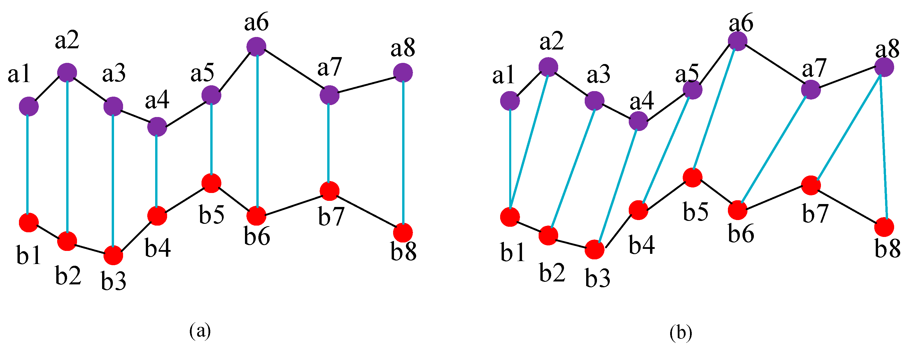
4.1. DTW Distance
- 1.
- Suppose two time series of data length m and n are A and B, where A = (a1, a2, …, am), B = (b1, b2, …, bn). Then, construct the data matrix C with m rows and n columns using A and B.
- 2.
- Define the bending path as P = {p1, p2, …, pk} and the Kth element of P as pk. The conditions to be satisfied by this dynamic bending path are as follows:
- A.
- Boundedness: max{m, n} ≤ k ≤ m + n − 1;
- B.
- Boundary conditions: p1 = c11, pm = cmn;
- C.
- Monotonicity and continuity: 0 ≤ i − i’ ≤ 1, 0 ≤ j − j’ ≤ 1.
- 3.
- Calculate the minimum dynamic bending distance of the two sequences:
4.2. Protection Scheme
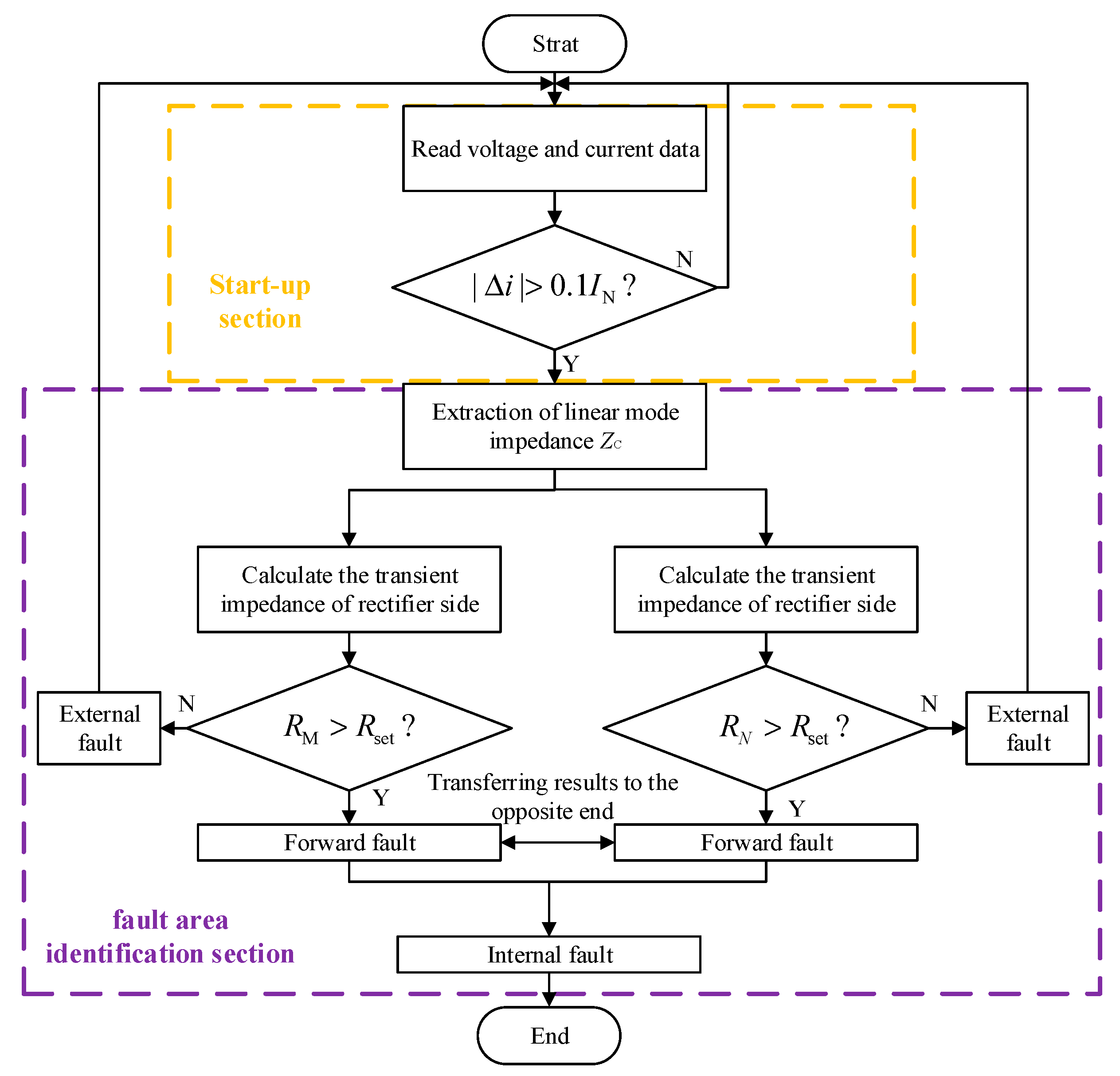
- (1)
- Program start: start reading fault voltage and current data.
- (2)
- Calculate whether the absolute value of the current increment is higher than the threshold value; if it is higher than the threshold value, then go to the next step, and otherwise return.
- (3)
- Extract ZC, which is calculated from the line parameters.
- (4)
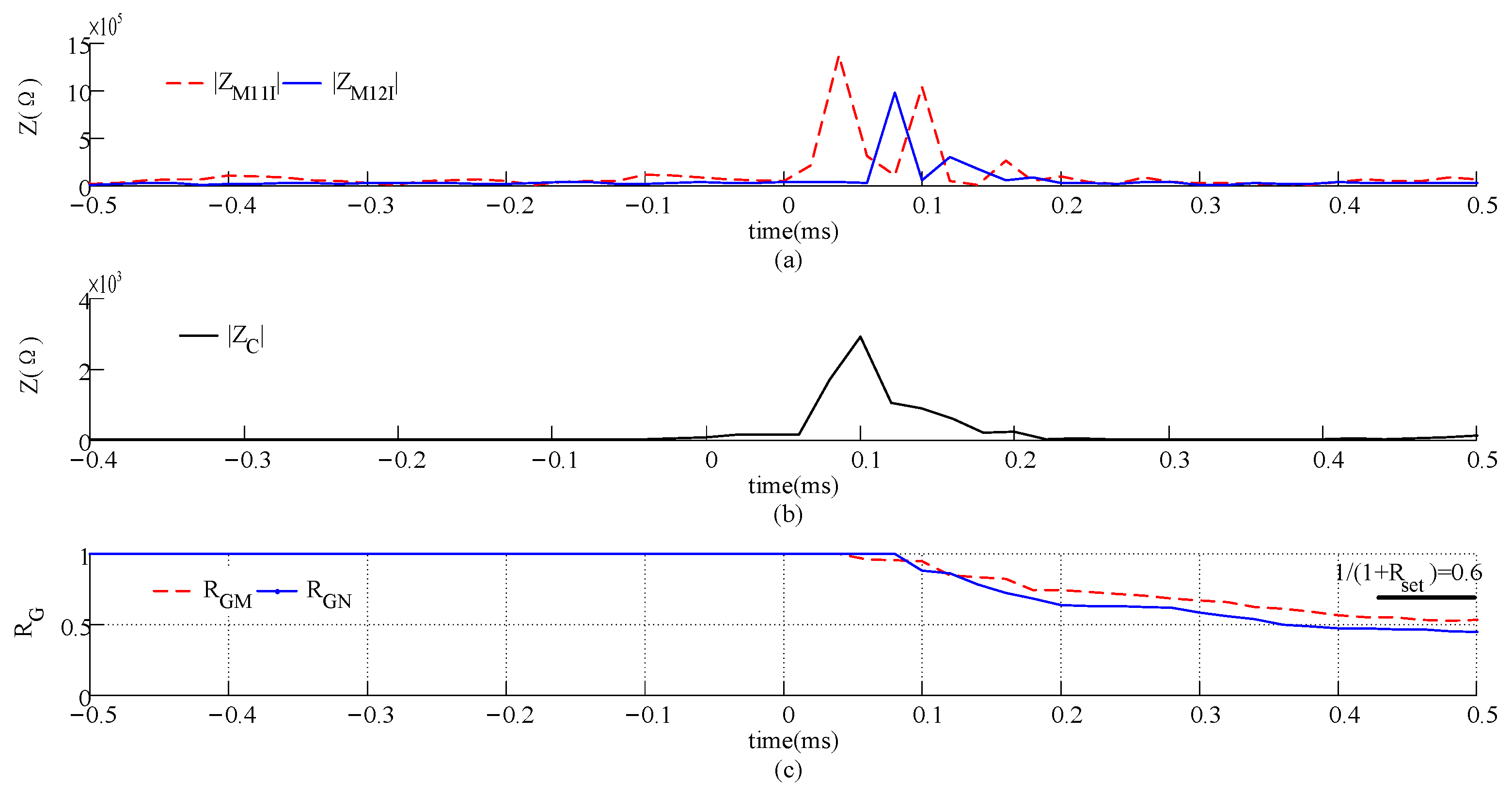
- Calculate the transient impedance and DTW distance on both sides of the line, respectively, and transmit the results to the opposite end. If the DTW distance on both sides is higher than the threshold value, it is judged that an internal fault occurs in the protection. To enhance the resistance to synchronization errors, forward faults are marked as 1, and reverse faults are marked as 0 for transmission to the opposite end.
- (5)
- End.
5. Simulation
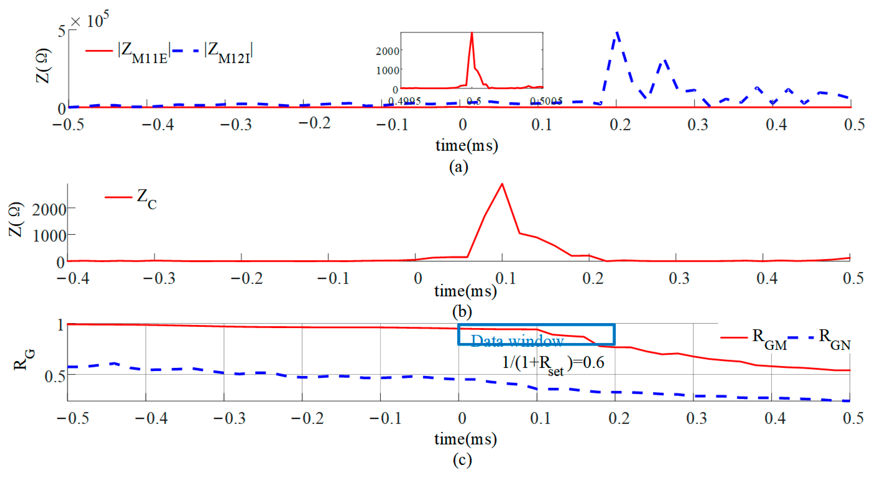
5.1. Correctness
- A.
- Internal fault
- B.
- External fault
5.2. Distributed Capacitance
5.3. Communication Delay
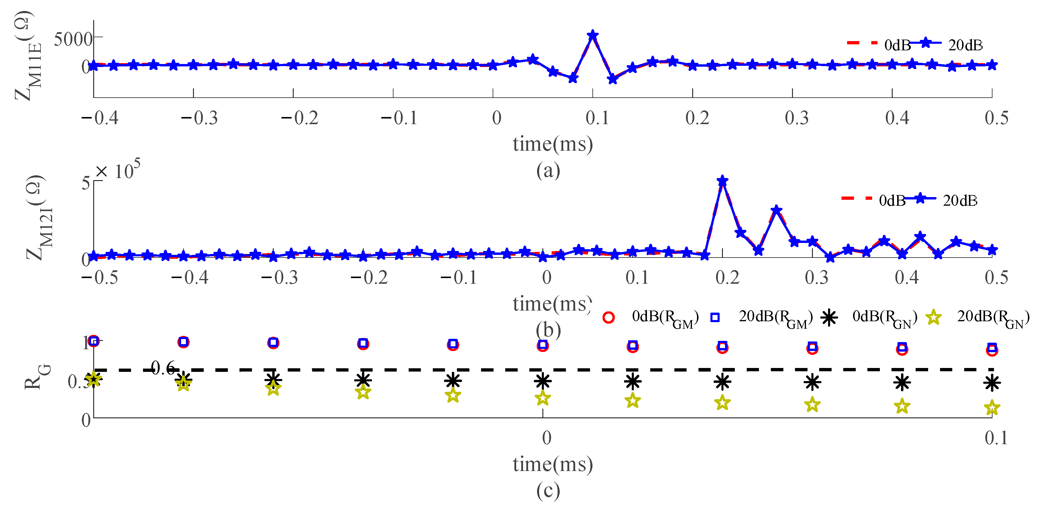
5.4. Fault Resistance and Noise
5.5. Performance Comparison
6. Conclusions
- (1)
- An expression for the transient impedance of a flexible DC distribution network containing distributed power is derived for the first time, and its fault characteristics are analyzed.
- (2)
- Compared with the traditional current differential protection and current direction protection, the use of transient impedance makes the scheme independent of the distributed capacitance and fault resistance.
- (3)
- The use of normalized DTW distances allows the scheme to accept longer communication delays than traditional waveform-matching-based schemes.
- (1)
- Although the simulation model in Figure 1 is derived from actual engineering, its reliability in complex environments still needs to be considered. For example, whether transient faults occurring frequently can be detected and whether the transformer can operate accurately when the error is large need to be determined. Therefore, the reliability verification of the proposed scheme under responsible working conditions is a direction for future research.
- (2)
- As the DC distribution grid is connected to a large number of distributed power sources, such as photovoltaics, wind power, electric vehicles, etc., the equivalent impedance of the system is bound to change. Therefore, studying the impedance characteristics of other distributed power sources is also a direction for future work.
Author Contributions
Funding
Institutional Review Board Statement
Informed Consent Statement
Data Availability Statement
Conflicts of Interest
Abbreviations
| DTW | dynamic time warping |
| DC | direct current |
| AC | alternating current |
| VSC | voltage source converter |
| ESS | energy storage system |
| PV | photovoltaic |
| ZVSC1 and ZVSC2 | converter impedance |
| ZL1, ZL2, ZL3, ZL4 | current-limiting reactor impedance |
| ZC | line wave impedance |
| ZDC | impedance of DC/DC converter |
| ZESS | impedance of energy storage |
| ZPV1 | impedance of PV |
| Uf1, Uf2, and Uf3 | fault voltage source |
| M11, M12 | circuit breaker for Line1 |
| M21, M22 | circuit breaker for Line2 |
| M31, M32 | circuit breaker for Line3 |
| M41, M42 | circuit breaker for Line4 |
| F1 | reverse external fault |
| F2 | internal fault |
| F3 | positive external fault |
| ZM11I | transient impedance of M11 of external fault |
| ZM11E | transient impedance of M11 of internal fault |
| ZM12I | transient impedance of M12 of external fault |
| ZM12E | transient impedance of M12 of internal fault |
| ZM31I | transient impedance of M31 of external fault |
| ZM31E | transient impedance of M31 of internal fault |
| ZM32I | transient impedance of M32 of external fault |
| ZM32E | transient impedance of M32 of internal fault |
| ZM21I, ZM22I, ZM41I and ZM42I | transient impedance of M21, M22, M41, and M42 |
| ZM21E, ZM22E, ZM41E and ZM42E | transient impedance of reverse fault |
| Uf(s) | fault voltage |
| If(s) | fault current |
| UfM (s) | measuring point voltage |
| IfM(s) | measuring point current |
| line propagation coefficient | |
| R, L, G, and C | resistance, inductance, conductance, and capacitance |
| R0 | equivalent resistance of the converter |
| Larm | equivalent inductance for bridge arms |
| Csm | equivalent capacitance of the converter |
| N1 | number of submodules |
| CDC | equivalent capacitance of the DC/DC converter |
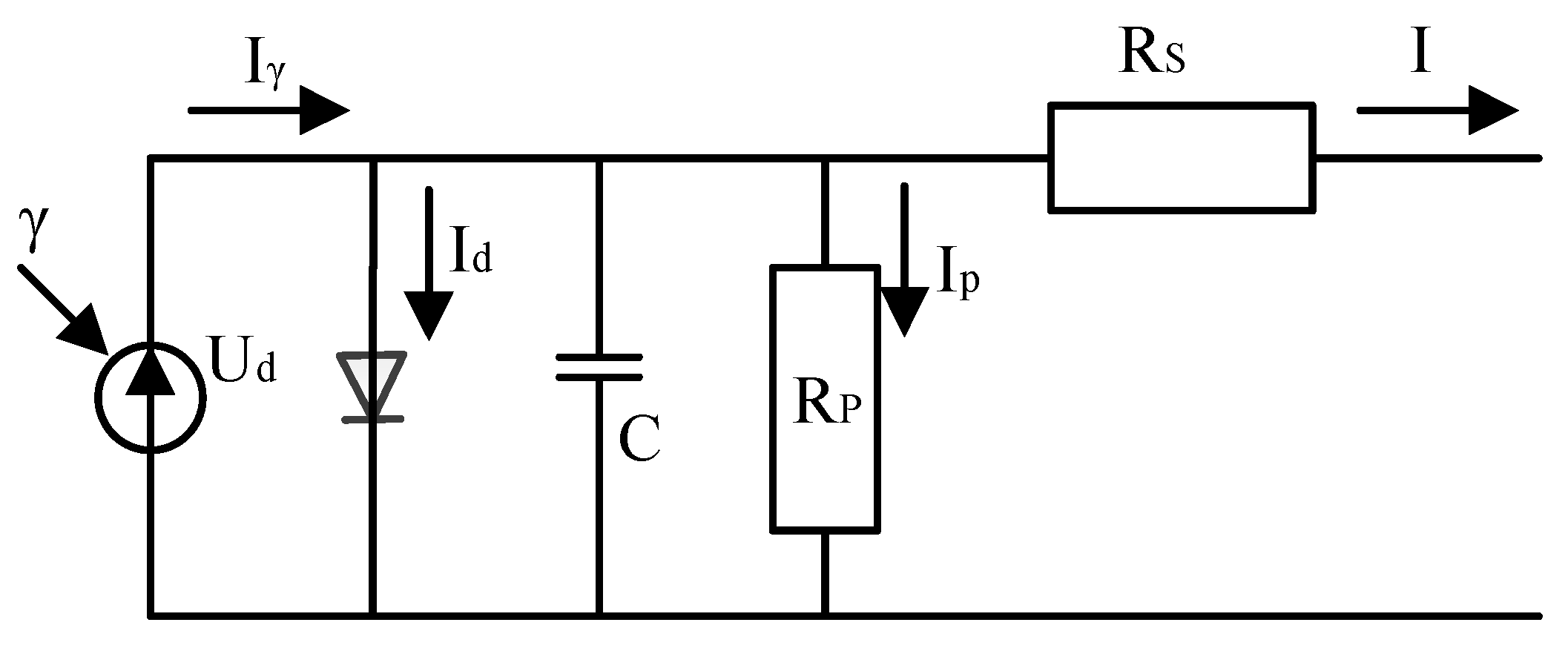
| Iγ | photogenerated current |
| γ | light intensity |
| Ud | junction voltage |
| I0 | reverse saturation current |
| Rs | series resistance |
| Rp | parallel resistance |
| U | load voltage |
| I | load current |
| A | ideal factor of the diode |
| K | Boltzmann constant |
| T | absolute temperature |
| q | electronic charge |
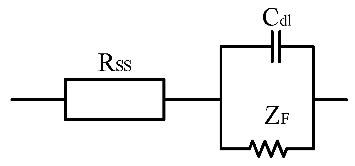
| RSS | solution resistance |
| Cdl | capacitance of the electrode to the electrolyte solution |
| ZF | Faraday impedance |
| n | stoichiometric coefficient |
| F | Faraday constant |
| Cs | electrode surface activity |
| D | diffusion coefficient |
| the number of reaction stages | |
| D(x,y) | Euclidean distance between the vector x(x1, x2) and the vector y(y1,y2) |
| C | data matrix |
| Rset | threshold value |
| RM and RN | DTW distances |
| ZMI | transient impedance |
| current increment | |
| IN | DC rated current |
| RGM\GN | normalized DTW distance |
| CDP [11] | current differential protection of [11] |
| CDP [12] | current differential protection of [12] |
| HSDPP | high-speed directional pilot protection |
| WMPP | waveform-matching pilot protection |
| HSCDP | high-sensitivity current differential protection |
| TIP | transient information protection |
References
- Baran, M.E.; Mahajan, N.R. DC distribution for industrial systems: Opportunities and challenges. IEEE Trans. Ind. Appl. 2003, 39, 1596–1601. [Google Scholar] [CrossRef]
- Wang, Y.; Song, Q.; Sun, Q.; Zhao, B.; Li, J.; Liu, W. Multilevel MVDC Link Strategy of High-Frequency-Link DC Transformer Based on Switched Capacitor for MVDC Power Distribution. IEEE Trans. Ind. Electron. 2017, 64, 2829–2835. [Google Scholar] [CrossRef]
- Castill-Calzadilla, T.; Cuesta, M.A.; Quesada, C.; Olivares-Rodriguez, C.; Macarulla, A.M.; Legarda, J.; Borges, C.E. Is a massive deployment of renewable-based low voltage direct current microgrids feasible? Converters, protections, controllers, and social approach. Energy Rep. 2022, 8, 12302–12326. [Google Scholar]
- Meghwani, A.; Srivastava, S.C.; Chakrabarti, S. A Non-unit Protection Scheme for DC Microgrid Based on Local Measurements. IEEE Trans. Power Deliv. 2017, 32, 172–181. [Google Scholar] [CrossRef]
- Aeishwarya, B.; Kaushik, D.; Matti, K.; Anca, D.H. Multi-Voltage Level Active Distribution Network With Large Share of Weather-Dependent Generation. IEEE Tran. Power Sys. 2022, 37, 4874–4884. [Google Scholar]
- Zhang, L.; Liang, J.; Tang, W.; Li, G.; Cai, Y.; Sheng, W. Converting AC converting AC distribution lines to DC to increase transfer capacity and DG penetration. IEEE Trans. Smart Grid 2019, 10, 1477–1487. [Google Scholar] [CrossRef]
- Li, B.; He, J.; Li, Y.; Li, R. A novel solid-state circuit breaker with selfadapt fault current limiting capability for LVDC distribution network. IEEE Trans Power Electron 2019, 34, 3516–3529. [Google Scholar] [CrossRef]
- Duan, J.D.; Li, Z.N.; Zhou, Y.; Wei, Z.Y. Study on the voltage level sequence of future urban DC distribution network in China: A Review. Int. J. Electr. Power Energy Syst. 2020, 117, 105640. [Google Scholar]
- Emhemed Abdullah, A.S.; Kenny, F.; Steven, F.; Graeme, M.B. Validation of fast and selective protection scheme for an LVDC distribution network. IEEE Trans. Power Deliv. 2017, 32, 1432–1440. [Google Scholar] [CrossRef]
- Wu, T.H.; Dai, W.; Li, X.D. Protection scheme and device development of flexible dc distribution network. Autom. Electr. Power Syst. 2019, 43, 123–130. [Google Scholar]
- Fletcher, S.D.A.; Norman, P.J.; Fong, K.; Galloway, S.J.; Burt, G.M. High-Speed Differential Protection for Smart DC Distribution Systems. IEEE Trans. Smart Grid 2014, 5, 2610–2617. [Google Scholar] [CrossRef]
- Song, G.; Cai, X.; Li, D.; Gao, S.; Suonan, J. A novel pilot protection principle for VSC-HVDC cable lines based on fault component current. In Proceedings of the 2012 Power Engineering and Automation Conference, Wuhan, China, 18–20 September 2012; pp. 1–4. [Google Scholar]
- Song, G.B.; Hou, J.J.; Guo, B. Pilot protection of flexible dc grid based on active detection. Power Syst. Technol. 2020, 5, 6. [Google Scholar]
- Li, B.; He, J.; Li, Y.; Li, B.; Wen, W. High-speed directional pilot protection for MVDC distribution systems. Int. J. Electr. Power Energy Syst. 2020, 121, 106141. [Google Scholar] [CrossRef]
- Song, G.B.; Luo, J.; Gao, S.P.; Wang, X.W.; Tassawar, K. Detection method for single-pole grounded faulty feeder based on parameter identification in MVDC distribution grids. Int. J. Electr. Power Energy Syst. 2018, 97, 85–92. [Google Scholar] [CrossRef]
- Shi, B.; Li, Y.; Sun, G. DC fault protection strategy for multi-terminal flexible DC distribution network based on full fault current information. High Voltage Eng. 2019, 45, 3076–3083. [Google Scholar]
- Qin, Y.; Wen, M.; Bai, Y.; Wang, Y.; Wang, X.; Fang, Z. A novel pilot protection scheme for HVDC lines based on waveform matching. Int. J. Electr. Power Energy Syst. 2020, 120, 106028. [Google Scholar] [CrossRef]
- Li, Z.; Zou, G.B.; Tong, B.B.; Gao, H.L.; Feng, Q. Novel traveling wave protection method for high voltage DC transmission line. In Proceedings of the 2015 IEEE Power & Energy Society General Meeting, Denver, CO, USA, 26–30 July 2015; pp. 1–5. [Google Scholar]
- Liu, J.; Tai, N.L.; Fan, C.J. Transient-voltage-based protection scheme for DC line faults in the multiterminal VSC-HVDC system. IEEE Trans. Power Deliv. 2017, 32, 1483–1494. [Google Scholar] [CrossRef]
- He, J.; Li, B.; Li, Y.; Qiu, H.; Wang, C.; Dai, D. A fast directional pilot protection scheme for the MMC-based MTDC grid. Proc. CSEE 2017, 37, 6878–6887. [Google Scholar]
- Liu, H.; Li, B.; Wen, W.; Green, T.C.; Zhang, J.; Zhang, N.; Chen, L. Ultra-fast current differential protection with high-sensitivity for HVDC transmission lines. Int. J. Elect. Power Energy Syst. 2021, 126, 106580. [Google Scholar] [CrossRef]
- He, Y.; Zheng, X.; Tai, N.; Wang, J.; Nadeem, M.H.; Liu, J. A DC line protection scheme for MMC-Based DC grids based on AC/DC transient information. IEEE Trans. Power Del. 2020, 35, 2800–2811. [Google Scholar] [CrossRef]


| Line Type | Parameter | Value and Unit |
|---|---|---|
| Wire | Wire radius | 0.0203454 (m) |
| DC resistance | 0.03206 Ω (km) | |
| Ground wire | Ground radius | 0.0055245 (m) |
| DC resistance | 2.8645 Ω (km) | |
| Ground resistivity | 100 Ω·m |
| Impedance Type | Frequency (Hz) | Impedance (Ω) |
|---|---|---|
| Line-mode wave impedance | 0.01 | 798.5 |
| 1 | 312.4 | |
| 100 | 256.7 | |
| 10,000 | 255.1 | |
| 1,000,000 | 254.5 | |
| Ground-mode wave impedance | 0.01 | 803.1 |
| 1 | 782.8 | |
| 100 | 650.8 | |
| 10,000 | 512.5 | |
| 1,000,000 | 455.3 |
| Forward | Reverse | Formula | |
|---|---|---|---|
| M11 | ZL1 + ZVSC1//(ZL2 + ZC) | ZC | ZVSC1,2,3,4 = 2/3R0 + 2/3sLarm + 1/(6Csm/N1) ZL1,2,3,4 = 2πfL ZC = [(R + sL)/(G + sC)]1/2 ZDC = ½πCDC ZESS = RSS + 1/(jωCdl + 1/ZF) |
| M12 | ZVSC2//(ZDC + ZESS)//(ZDC + ZPV1)//(ZL3 + ZC) | ||
| M21 | ZL1 + ZVSC1//(ZL1 + ZC) | ||
| M22 | ZVSC1//(ZDC + ZPV2)//(ZDC + ZPV3)//(ZL4 + ZC) | ||
| M31 | ZVSC1//(ZDC + ZESS)//(ZDC + ZPV1)//(ZL1 + ZC) | ||
| M32 | ZL3 + ZVSC1//(ZL4 + ZC) | ||
| M41 | ZVSC1//(ZL2 + ZC)//(ZDC + ZPV2)//(ZDC + ZPV3) | ||
| M41 | ZL4 + ZVSC2//(ZL3 + ZC) |
| Communication Delay (ms) | RGM | RGN | Result |
|---|---|---|---|
| 0.1 | 0.987 | 0.979 | Operation |
| 0.2 | 0.975 | 0.963 | |
| 0.3 | 0.874 | 0.820 | |
| 0.4 | 0.941 | 0.917 | |
| 0.5 | 0.915 | 0.845 |
| Fault Resistance (Ω) | RGM | RGN | Result |
|---|---|---|---|
| 10 | 0.991 | 0.966 | Operation |
| 20 | 0.932 | 0.950 | |
| 30 | 0.917 | 0.901 | |
| 40 | 0.981 | 0.947 | |
| 50 | 0.975 | 0.950 |
| Conditions | Proposed | CDP [11] | CDP [12] | HSDPP [14] | WMPP [17] | HSCDP [21] | TIP [22] |
|---|---|---|---|---|---|---|---|
| Time (ms) | 0.3 | 20 | 15 | 2 | 2 | >3.01 | 5 |
| Fault resistance (Ω) | 50 | 50 | 50 | 100 | 100 | 100 | 100 |
| Sampling frequency (kHz) | 50 | 10 | 10 | 50 | 10 | 10 | 20 |
| Noise (dB) | 20 | 30 | 30 | 30 | 20 | 30 | 30 |
| Communication delay (ms) | 0.5 | 0.1 | 0.3 | 0.1 | 0.2 | 0.2 | 0.1 |
| Distributed capacitance (times) | 10 | 3 | 5 | 6 | 5 | 7 | 4 |
Disclaimer/Publisher’s Note: The statements, opinions and data contained in all publications are solely those of the individual author(s) and contributor(s) and not of MDPI and/or the editor(s). MDPI and/or the editor(s) disclaim responsibility for any injury to people or property resulting from any ideas, methods, instructions or products referred to in the content. |
© 2023 by the authors. Licensee MDPI, Basel, Switzerland. This article is an open access article distributed under the terms and conditions of the Creative Commons Attribution (CC BY) license (https://creativecommons.org/licenses/by/4.0/).
Share and Cite
Ni, P.; He, J.; Wu, C.; Zhang, D.; Yuan, Z.; Xiao, Z. Protection Scheme for Transient Impedance Dynamic-Time-Warping Distance of a Flexible DC Distribution System. Sustainability 2023, 15, 12745. https://doi.org/10.3390/su151712745
Ni P, He J, Wu C, Zhang D, Yuan Z, Xiao Z. Protection Scheme for Transient Impedance Dynamic-Time-Warping Distance of a Flexible DC Distribution System. Sustainability. 2023; 15(17):12745. https://doi.org/10.3390/su151712745
Chicago/Turabian StyleNi, Pinghao, Jinghan He, Chuanjian Wu, Dahai Zhang, Zhaoxiang Yuan, and Zhihong Xiao. 2023. "Protection Scheme for Transient Impedance Dynamic-Time-Warping Distance of a Flexible DC Distribution System" Sustainability 15, no. 17: 12745. https://doi.org/10.3390/su151712745
APA StyleNi, P., He, J., Wu, C., Zhang, D., Yuan, Z., & Xiao, Z. (2023). Protection Scheme for Transient Impedance Dynamic-Time-Warping Distance of a Flexible DC Distribution System. Sustainability, 15(17), 12745. https://doi.org/10.3390/su151712745