Safety Evaluation Method for Submarine Pipelines Based on a Radial Basis Neural Network

Abstract

As the lifeline of offshore oil and gas production, a submarine pipeline requires regular safety evaluations with proper maintenance according to the evaluation results. At present, the safety factors based on regional-level commonly used factors in engineering are too many, and this leads to conservative evaluation results with a low acceptance of defects. In this paper, a risk factor evaluation index system for submarine pipeline defects is constructed through an analytic hierarchy process (AHP), and the original safety factors are corrected to achieve accurate evaluations for submarine pipeline safety. By constructing a radial basis neural network (RBFNN), the fast calculation of safety factors for other pipeline defects can be realized. Through comparison, it was found that the values obtained by the machine training were in good agreement with the real values, which reflects the accuracy of the model and provides a basis for the repair of a defective pipeline.

1. Introduction

A submarine pipeline is an important means of offshore oil and gas transportation and the lifeline of offshore energy transportation [1,2]. Generally speaking, a submarine pipeline system is composed of large steel submarine pipelines, pumping stations, a power supply, and communication systems, which, together, are responsible for closely linking and combining the entire production of offshore oil and gas fields. They have received extensive attention and have applications all over the world [3]. Since the Brown and Root Offshore Engineering Company of the United States laid the world’s first submarine pipeline in the Gulf of Mexico in 1945 [4], other countries have successively carried out the work of laying submarine pipelines in major sea areas. The world’s large offshore oil and gas fields, including Iran’s Shashan Oilfield, the Efesk Oilfield in the Norwegian Sea, and the Fortis Oilfield in the British Sea, all use submarine pipelines for crude oil transportation. Since China built the first submarine oil pipeline in the Chengbei Oilfield in the Bohai Sea in 1985, more than 80 oil and gas fields have been built in different sea areas. There are nearly 100 pipelines of various specifications, with a total length of more than 4000 km [5].

Although submarine pipeline transportation has the advantages of large and stable transportation, low investment, quick results, safe sealing, and easy remote centralized management, compared with land oil and gas pipelines, the service conditions of submarine pipelines are more stringent and their monitoring and maintenance are more difficult [6]. Once an accident occurs, it causes huge losses to the oil field and also pollutes the environment [7]. The safety evaluation of a submarine pipeline in actual engineering is primarily based on relevant specifications, and judgments are made based on factors such as pipeline internal pressure and defect size. Therefore, more and more attention has been paid to how to evaluate the safety of an in-service submarine pipeline quickly and accurately [8].

In the 1990s, based on the local response characteristics of biological neurons and the research results of radial basis functions, Broomhead and Lowe introduced radial basis functions into the construction of neural network models, forming a radial basis neural network [9]. The basic idea of a radial basis function (RBF) neural network is to transform input data by using a radial basis function provided by the hidden units in the network as the “basis”. The input data is transformed from a low-dimensional linearly separable pattern to a suitable high-dimensional linearly separable space, and then the hidden units are weighted and summed to obtain the output units. This provides a reasonable solution to the problem of linear indivisibility in low-dimensional spaces [10].

This paper takes an actual marine pipeline as the research object, considering the ASME standard. The safety factor in B 31 G is used as the basis for defect evaluation, and, combined with the defect-related risk factors, the safety factor is corrected and an evaluation that can better reflect the safety state of the defect is made. At the same time, in order to simplify the evaluation process, this paper realizes the rapid calculation of the safety factor of a submarine pipeline by constructing and training an RBFNN. The size of the revised safety factor provides a theoretical basis for the planned maintenance and repair of the pipeline, and it provides a technical guarantee for the safe operation of the submarine pipeline.

2. Research Status of the Safety Evaluation Method for a Marine Pipeline

Due to the large number of factors affecting pipeline integrity and their different mechanisms of influence, it is difficult to evaluate the effect of each factor quantitatively. Many scholars have introduced different methods to describe the influencing factors and take the influence of each factor into account in the safety evaluation.

Xu Haitao [11] analyzed oil pipe corrosion data using a gray correlation analysis method, calculating the factors that could be quantitatively described and evaluating residual strength on the basis of a force analysis. Han Xiaoming [12] ranked the importance of influencing factors and used an artificial neural network to predict the remaining life and detection cycle of a pipeline. Luo Zhengshan [13] carried out a gray correlation analysis to select important influencing factors and build a corrosion prediction model based on a gray support vector machine. Sun Baocai [14] determined the influencing factors of pipeline failure pressure through a sensitivity analysis and established a GA-BP (L-M) prediction model. Senouci [15] developed regression analysis and artificial neural network (ANN) prediction models based on historical pipeline accident data to predict pipeline accidents.

At present, there are few studies that have researched the impacts of risk factors on a submarine pipeline’s integrity. This paper aims to fill the gap in the field and integrate the influence of various risk factors into the original pipeline safety evaluation method. A radial basis neural network with a simpler structure and a faster convergence speed is used to evaluate the safety of a submarine pipeline.

3. Research on the Safety Factors in Submarine Pipeline Defects

Since the 1960s, some Western developed countries have been conducting research on the evaluation of subsea oil and gas pipelines with defects. Thus far, led by the United States, Canada, and some European countries, the ASME B 31 G standard, the RS TRENG standard, the DNV RP-F101 standard, the API579 standard, the elastic limit criterion, the plastic failure criterion, the finite element method, the AGA NG-18 method, the PRORRC method, the ultimate load analysis method, the reliability theory, and other pipeline integrity methods have been developed. These methods have their own scope of application and conservatism [16]. This article only gives a brief introduction to the ASME B31G code.

The ASME B31 G standard has issued four versions so far, namely the ASME B31G-1984 [17] standard, the ASME B31G-1991 [18] standard, the ASME B31 G-2009 [19] standard, and the ASME B31 G-2012 standard [20], among which the ASME B31G-1984 standard, also known as the concise evaluation method for the residual strength of corroded pipelines, is one of the most widely used standards in Europe and the United States. The ASME B31G-1991 standard has partially amended and improved the ASME B31G-1984 standard [18]. Based on many experimental data points, the ASME B31G-2009 standard has significantly changed the ASME B31G-1991 standard. This revision will overcome the conservatism of the ASME B31G-1991 standard. However, Nova Corporation in Alberta, Canada, and Pipeline Company in the UK subsequently demonstrated through research methods such as blasting experiments that the ASME B31G standard still has conservatism in evaluating corrosion defects in pipelines. It is also pointed out that one of the reasons for the conservatism of the ASME B31 G standard is that the impact of single corrosion defects, double corrosion defects, interaction corrosion defects, and corrosion defects with a spiral angle are all evaluated according to the same evaluation method. To solve this problem, ARCO Alaska Co., Ltd. proposed a highly approximate condition for treating discontinuous and multiple corrosion defects as one corrosion defect.

The ASME B31G evaluation method is based on a semi-empirical formula and the NG-18 formula of fracture mechanics. This evaluation method has significant computational advantages, as it can quickly calculate the predicted circumferential failure pressure with defects and the circumferential stress under operating pressure and evaluate them in conjunction with safety factors. This standard believes that defects are acceptable when the predicted circumferential failure pressure is greater than or equal to the product of the safety factor of the pipeline and the circumferential stress under operating pressure, as shown in Formula (1):

$$S_F\ge SF\times S_0$$

(1)

$$S_F=S_{flow}[\frac{1-A/A_0}{1-(A/A_0)/M}]$$

(2)

$$S_0=(MAOP\times D)/2t$$

(3)

In the formula, S_F is the predicted circumferential failure stress, MPa; A₀ is the pipe wall area at the defect location, mm²; A is the projected area of the defect section, mm²; M is the expansion coefficient; S_flow is the flow stress of the material, MPa; SF is the safety factor of the pipeline; S₀ is the hoop stress under the operating pressure, MPa; MAOP is the maximum allowable operating pressure, MPa; D is the outer diameter of the pipeline, mm; t is the wall thickness of the pipeline, mm.

3.1. Safety Factor Based on Regional-Level

This article ultimately selects the safety factor in ASME B31G as the main parameter for evaluating the integrity of submarine pipelines. The Safety Factor is a coefficient used in engineering structural design methods to reflect the degree of structural safety. To prevent consequences caused by factors such as material defects, work deviations, and sudden increases in external forces, the theoretical force that the stressed part of the project can bear must be greater than the actual force it bears, that is, the ratio of predicted failure pressure to operating pressure. The ratio of the two is called the safety factor, and the calculation formula is shown in Formula (4).

$$SF=\frac{p_F}{p_0}$$

(4)

$$p_F=\frac{p}{F}$$

(5)

In the formula, p_F is the predicted failure pressure based on the regional level, MPa; p₀ is the operating pressure, MPa; p is the design pressure, MPa; F is the design coefficient, and the value is related to the regional level.

Since the submarine pipelines’ operating pressure values differ under different working conditions, this paper subsequently evaluates the most dangerous working conditions, where p₀ is the maximum allowable operating pressure value. In most cases, the design pressure of domestic submarine long-distance pipelines is equal to the maximum allowable operating pressure, so the formula for calculating the safety factor can be simplified to the reciprocal of the design factor, as shown in Formula (6).

$$SF=\frac{1}{F}$$

(6)

Combining the design coefficient values based on regional levels in the ASME B31G code and the classification criteria for subsea pipeline regional levels in the DNV 2000 subsea pipeline system code, a table for assigning submarine pipeline design coefficients can be established, as shown in

Table 1. Design coefficient assignment table for the submarine pipeline.

Submarine Pipeline Regional-Levels	Division Basis	Design Factor
Level 1 area	Occasionally pass through the route, but there is no impact due to surging ocean currents	0.72
Level 2 area	The passage of the route is small, and the impact of ocean current surges is not large	0.6
Level 3 area	Passages are frequent, and the impact of ocean currents is large	0.5
Level 4 area	The passage is widespread, and the ocean currents are turbulent and impactful	0.4

.

3.2. Calculation of the Risk Score Based on AHP

The AHP method is a set of advantages of qualitative and quantitative analysis [21], which is a mathematical evaluator’s evaluation thinking process for complex systems and can solve multiple problems simultaneously. Decision makers initially determine the importance ranking of each criterion based on experience and use corresponding algorithmic programs to calculate the weights of each criterion. By using specific weights, the relationship of relative importance between each criterion and another, as well as between a specific criterion and the overall goal, can be accurately expressed, which is especially suitable for structural models with complex standard structures and relatively scarce necessary data [22].

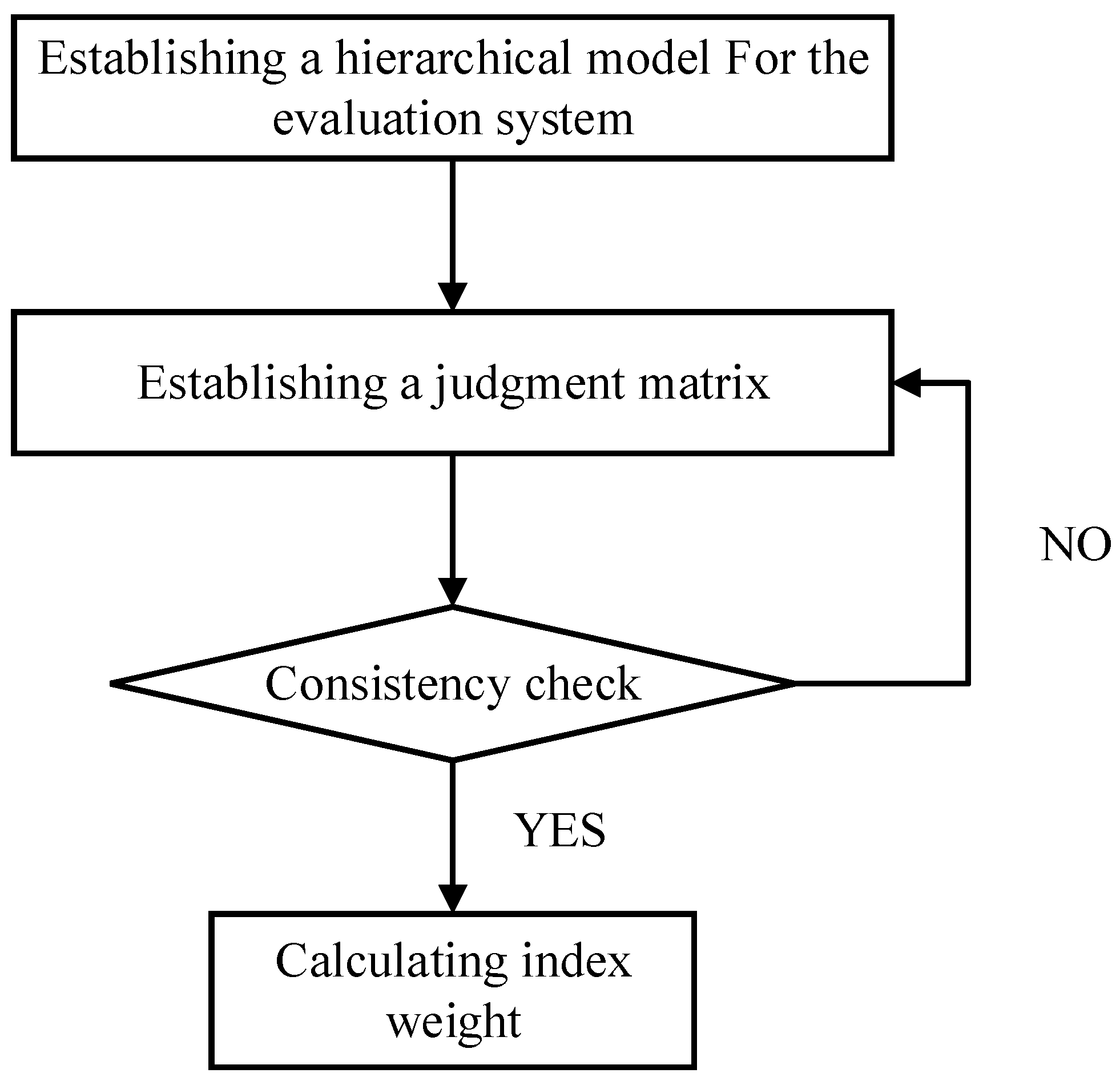
The AHP mainly considers the empirical knowledge and personal preferences of experts. Its basic principle is to compare and judge the evaluation index models at the same level in pairs based on relevant criteria, determine the evaluation matrix, and then conduct consistency testing. The matrix is modified until it passes the consistency test. Finally, the maximum eigenvalue and eigenvector of the judgment matrix are calculated as the subjective weights of the evaluation index. In addition, as the evaluation indicators increase, the order also increases, making it relatively difficult to compare the indicators in pairs and challenging to pass the consistency test. Therefore, 1 to 9 are generally chosen to illustrate their relative importance [23]. The specific analysis flowchart is shown in Figure 1.

(1)

Establish a hierarchical model of the evaluation system

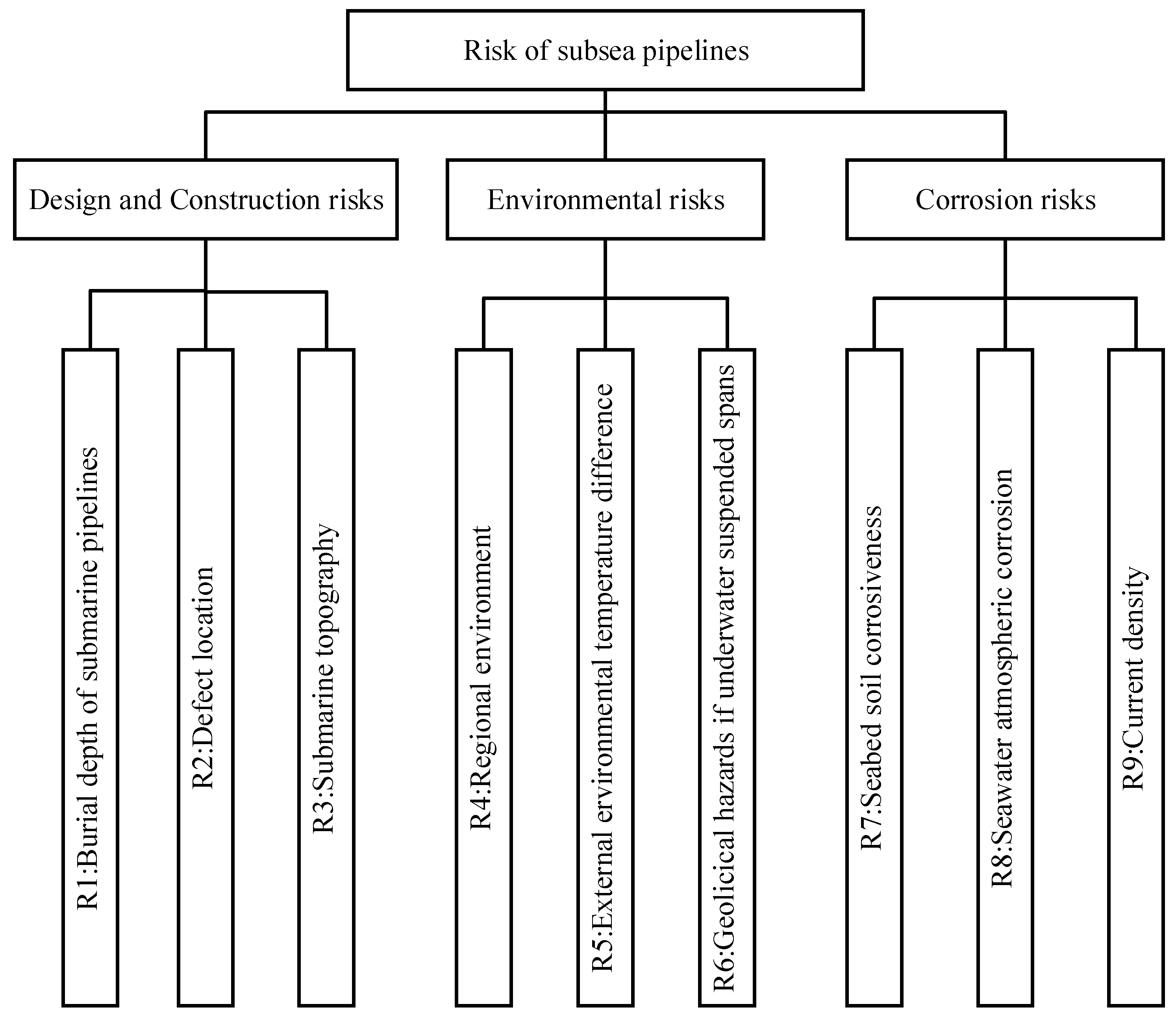
To study the defects contained in pipelines, it is initially necessary to clarify the risk factors related to subsea pipelines. After reviewing relevant literature and analyzing the causes of pipeline accidents both domestically and internationally [24,25,26], based on the applicable standard GB-T 27512-2011 “Risk Assessment Method for Buried Steel Pipelines” [27] and the actual situation, this article selects a total of nine risk factors from three aspects to develop an evaluation system hierarchical model, as shown in Figure 2.

For easy reading of subsequent forms, nine risk factors are named from R1 to R9, as shown in Figure 2.

(2)

Experts score and establish a judgment matrix

According to the experience and knowledge of experts, the factors of the same layer are compared in pairs to determine the relative importance of the two factors.

Table 2. Judgment Matrix Construction Standards.

Relative Importance aij	Definition	Explanation
3	Slightly important	Goals i and j are slightly more important
5	Quite important	Goals i and j are quite important
7	Obviously important	Goals i and j are clearly important
9	Absolutely important	Goals i and j are absolutely important
2, 4, 6, 8	Between two levels of importance

shows the importance-assigning criteria.

This table adopts a five-level quantitative method for representing the relative importance of one indicator to another. On the contrary, the other indicator is secondary to this indicator, represented by the reciprocal of the corresponding value. At the same time, to improve the accuracy of the judgment matrix, four numbers, 2, 4, 6, and 8, were introduced between 1, 3, 5, 7, and 9, respectively, to construct the judgment matrix. The relative importance of each risk factor is shown in

Table 3. Risk Factor Importance.

Risk Matrix	R1	R2	R3	R4	R5	R6	R7	R8	R9
R1	1	6/5	6/9	1	6/5	6/8	6/4	6/5	6/7
R2	5/6	1	5/9	5/6	1	5/8	5/4	1	5/7
R3	9/6	9/5	1	9/6	9/5	9/8	9/4	9/5	9/7
R4	1	6/5	6/9	1	6/5	6/8	6/4	6/5	6/7
R5	5/6	1	5/9	5/6	1	5/8	5/4	1	5/7
R6	8/6	8/5	8/9	8/6	8/5	1	8/4	8/5	8/7
R7	4/6	4/5	4/9	4/6	4/5	4/8	1	4/5	4/8
R8	5/6	1	5/9	5/6	1	5/8	5/4	1	5/7
R9	7/6	7/5	7/9	7/6	7/5	7/8	8/4	7/5	1

.

(3)

Consistency check of the judgment matrix

To verify whether the calculated results are consistent with the evaluation criteria, determine whether they can be directly used for further analysis of the problem, and prevent irrelevant factors outside the system from interfering with the judgment matrix and causing deviations in the calculation results, it is necessary to verify whether the preliminary calculation results are consistent. Only when the judgment matrix basically meets the consistency test [28] can the next related operation be carried out, and the consistency test shows that the weight scale assignments in the judgment matrix are reasonable and not contradictory to each other, so that further relevant analysis of the problem can be carried out. The calculation formula for consistency check [29] is shown in Formula (7):

$$CR=\frac{CI}{RI}$$

(7)

In the formula, CR is the consistency ratio, and its specific meaning is that when the value of CR is less than 0.10, it indicates that the consistency corresponding to the judgment matrix is within an acceptable range. Otherwise, it is necessary to change the corresponding importance assignment in the judgment matrix, correct it to a value that matches the actual importance, and bring it into the matrix until it finally meets the consistency check.

CI is an indicator of consistency, and the calculation method is shown in Formula (8):

$$CI=\frac{{\lambda }_{\max }-n}{n-1}$$

(8)

In the formula, the maximum eigenvalue of the judgment matrix is λ_max and the order is n. In Formula (7), RI is the average random consistency index related to the order n, and the corresponding value of RI can be found in

Table 4. Random Consistency Index (RI).

Matrix Order	1	2	3	4	5	6	7	8	9	10
RI	0	0	0.52	0.89	1.12	1.26	1.36	1.41	1.46	1.49

.

(4)

Calculate the subjective weight of the evaluation index

Taking the judgment matrix A as an example, the eigenvectors and eigenvalues of A are calculated, as shown in Formula (9) [30]:

$$A{W}^{\prime }={\lambda }_{\max }{W}^{\prime }$$

(9)

The weight of each influencing factor λ_max is the characteristic root of the judgment matrix A.

The weight calculation results of each risk factor in the hierarchical model of the evaluation system constructed in this section are shown in

Table 5. Risk Factor Weights.

Risk Factors	Weights
Pipeline depth	0.11
Defect location	0.09
Seabed topography	0.16
Regional Environment	0.11
External ambient temperature difference	0.09
Submarine Suspended Geological Hazards	0.15
Soil corrosion	0.07
Atmospheric corrosion	0.09
Current density	0.13

.

Based on the weight of each risk factor, the establishment of the scoring rules for each indicator can be carried out as follows:

(1)

Design and construction risks (36 points)

① Burial depth of a submarine pipeline (11 points): If it is a crossing or exposed section, the score is 0 points. If it is a buried pipeline section, the score calculation for the burial depth of non-underwater crossing pipelines is shown in the Formula (10).

$$Min(\frac{d}{145},11)$$

(10)

In the formula, d is the actual thickness of the overburden layer.

② Defect location (9 points): If it is located in many areas where waterways or rivers intersect, 0 points will be given. If it is located in a mixed area of the waterway, the score is 4.5 points. If it is far from the waterway area, the score will be 9 points.

③ Submarine topography (16 points): 0 points for ocean trenches; 6 points for mid-ocean ridges and ocean basin edges; 10 points for continental slopes and continental uplifts; 16 points for continental shelves, abyssal plains, the middle of ocean basins, etc.

(2)

Environmental risk (35 points)

① Regional environment (11 points): If there is an area with high tides and dense waterways and the pipeline passes through this area, 4 points will be given. If the pipeline is located in areas with high tides and frequent passage of waterways, 7 points will be given. If the pipeline environment is located at low tide and the waterway is not dense, 9 points will be given. If the pipeline environment is located in a stable tidal and non-navigable area, 11 points will be given.

② External environment temperature difference (9 points): If the average temperature difference between winter and summer in the external environment is greater than 20 degrees, 3 points will be given. If the average temperature difference between winter and summer in the external environment is greater than 15 degrees, 5 points will be given. If the average temperature difference between winter and summer in the external environment is 0–15 degrees, a score of 9 points will be given.

③ Submarine suspended-span geological disasters (15 points): The score is 6 points if a submarine earthquake, seabed movement, ice disaster, and other natural disasters occur frequently; 12 points for occasional submarine earthquakes, seabed movements, ice disasters, and other natural disasters; and 15 points for almost no natural disasters such as submarine earthquakes, seabed movements, and ice disasters.

(3)

Corrosion risk (29 points)

① Seabed soil corrosiveness (7 points): If the soil resistivity is less than 20 Ω·m, the score is 0 points. If the soil resistivity ∈ [20 Ω·m, 50 Ω·m], then it is 4 points. If the soil resistivity is >50 Ω·m, it is 7 points.

② Seawater atmospheric corrosion (9 points): If the defect is located in the riser section without protection, the score for atmospheric corrosion is 3 points. If no marine atmospheric corrosivity survey has been conducted, 0 points will be given. If it is an offshore riser section with good protection, 6 points will be given. When the defect is located in the seabed section, the score for atmospheric corrosion is 9 points.

③ Current density (13 points): 0 points for current density > 20 μA/mm²; 2 points for current density ∈ (10 μA/mm², 20 μA/mm²); 6 points for current density ∈ (2 μA/mm², 10 μA/mm²); 9 points for current density ∈ (0.5 μA/mm², 2 μA/mm²); 13 points for current density ≤ 0.5 μA/mm².

3.3. Safety Factor Correction

The submarine pipeline system includes many business departments, and the system’s efficient operation depends on the unity and cooperation of various departments. The shared platform for achieving mutual communication and correlation, which uses the Geographic Information System (GIS) for collecting different business information, is based entirely on the spatial distribution characteristics of data and resources within the pipeline transportation system. The combination of electronic maps and pipeline transportation makes it possible to comprehensively and intuitively reflect the current status, distribution, and technical characteristics of transportation objects, transportation tools, and their related information. Therefore, it maximizes the sharing of information and data, providing a reference basis and auxiliary decision-making support for the operation and management of pipeline transportation.

The data used in this article are all from the monitoring and recording of a submarine pipeline using the Pipeline Geographic Information System. The pipeline adopts X60 pipe steel with a diameter of 660 mm and a designed working pressure of 6.4 MPa. The collected data includes relevant data on defects as well as attribute data such as the burial depth of the submarine pipeline at the defect location, seabed terrain, external environmental temperature difference, soil corrosion properties, and current density.

Normalize the risk scores at the defect points of each submarine pipeline using a self-designed program, and then modify the safety factor based on the regional level. The correction formula is shown in Formula (11):

$$S{F}_1=S{F}_0\times x/100$$

(11)

In this formula, SF₁ is the revised safety factor; SF₀ is the safety factor based on the regional level; and x is the risk score.

A self-designed program calculates the predicted circumferential failure stress (S_F) mentioned in this article and combines it with the pipeline’s design pressure and safety factor to determine whether the defect is acceptable.

Table 6. Comparison of evaluation results.

Serial Number	Risk Score	SF (MPa)	Factor of Safety Based on Regional Classes	Original Evaluation Result	Modified Safety Factor	The Revised Evaluation Result
1	74.52	9.54	1.67	unacceptable	1.24	acceptable
2	77.97	9.66	1.67	unacceptable	1.30	acceptable
3	81.28	9.79	1.67	unacceptable	1.36	acceptable
4	61.71	9.79	1.67	unacceptable	1.03	acceptable
5	79.03	9.73	1.67	unacceptable	1.32	acceptable
6	70.31	9.86	1.67	unacceptable	1.17	acceptable
7	66.12	9.73	2	unacceptable	1.32	acceptable
8	84.03	9.66	1.67	unacceptable	1.40	acceptable
9	75.72	9.73	1.67	unacceptable	1.26	acceptable
10	74.21	9.66	1.67	unacceptable	1.23	acceptable
11	69.52	9.60	1.67	unacceptable	1.16	acceptable
12	77.97	9.60	1.67	unacceptable	1.30	acceptable
13	73.90	9.73	1.67	unacceptable	1.23	acceptable
14	68.40	9.79	1.67	unacceptable	1.14	acceptable

compares the evaluation results based on the original and modified safety factors for some submarine pipeline defects.

It can be seen from the above table that after considering the correction of various risk factors at the defect zone, the problem of the original evaluation results being too conservative has been improved, providing a new theoretical basis for the safety evaluation of submarine pipelines.

4. Research on the Calculation Model of the Safety Factor by RBFNN

Based on the revision of the safety factor in the previous text, to further improve the speed and efficiency of safety evaluation for submarine pipelines, a safety factor calculation model based on RBFNN has been established.

4.1. Radial Basis Neural Network

The RBF network has the advantages of a simple structure, fast convergence [31], and the ability to approximate any nonlinear function. As a forward network composed of three layers, the first layer of the RBFNN is the input layer, and the number of nodes is equal to the input dimension. The second layer is the hidden layer, and the number of nodes depends on the complexity of the problem. The third layer is the output layer, with the number of nodes equal to the dimension of the output data. Different layers have different functions. The hidden layer is nonlinear. The radial basis function is used as the basis function so that the input vector space can be transformed into the hidden layer space, making the original linear indivisible problem linear and separable.

The steps to determine the pipeline safety factor using an RBFNN in this section are:

(1)

Define the input vectors and their target output values for each sample based on the data provided in the table.

(2)

Divide training data and testing data.

(3)

To fully utilize the training samples, two-dimensional interpolation is performed on the training samples to increase the sample data size to four times the original size.

(4)

Create and train RBFNN.

(5)

Use the created RBFNN model to test the samples.

4.2. Models Based on Radial Basis Function Neural Networks

Based on existing data, the model adopts relevant risk factors as independent variables, namely the buried depth of the pipeline at the defect location, defect location, seabed terrain, regional environment, external environmental temperature difference, geological disasters, soil corrosiveness, atmospheric corrosion, current density, and the modified safety coefficient as dependent variables, forming a functional relationship as shown in Formula (12):

$$y=f(x_1,x_2,x_3,\cdots x_9)$$

(12)

where x₁~x₉ represent the above nine independent variables, respectively, and y is the defect safety factor proposed in this paper.

To fully utilize the training samples, this article performs a two-dimensional difference on the training samples to increase the sample data by four times. Based on the sorted data, define the sample’s input vector and the target’s output vector, and use 1/10 of the data as test data and 9/10 groups as training data. The model is obtained by training the training data, and then the test data is used to verify the model.

When creating an RBFNN, the number of nodes in each network’s hidden layer differs, so users need to adjust the error target according to their actual situation; the function will add new hidden layer nodes to the network based on different error target values while adjusting the node center, standard deviation, and weight values to ensure that the network meets the set error requirements. In the network model set up in this article, the error tolerance is 1 × 10⁻⁶, the diffusion factor is 38, and the maximum number of neurons is 300.

The corresponding relationship between the number of specific neuron nodes and the training error value is shown in

Table 7. Training error values.

Number of Neurons	0	50	100	150	200	250
training error value	0.0061677	0.0061677	9.62773 × 10−6	3.6752 × 10−6	2.05146 × 10−6	1.23123 × 10−6

.

The RBFNN diagram constructed in this paper is shown in Figure 3. It can be seen from the figure that the network structure includes 12 input nodes, 269 hidden layer nodes, and 1 output node.

4.3. Test Results

By using the created model to test the test dataset, the corresponding relationship between the predicted values and the true values can be shown in Figure 4.

The residual between the predicted and actual values is shown in Figure 5. The figure shows that the test value of the defect safety factor is in good agreement with the actual value, with a maximum residual of 0.17, which does not exceed 6%. This value can be tested and, to some extent, reflects the model’s accuracy.

5. Conclusions

This article established an evaluation index system for the risk factors of submarine pipeline defects using the AHP, which corrects the safety factor based on the regional level and overcomes the problem of the original evaluation results being too conservative. Based on the revised safety factor, an RBFNN is created and trained to rapidly calculate the safety factor of submarine pipelines. The following points can be highlighted:

(1)

The safety factor evaluation method in ASME B31G is selected as the basis for the safety evaluation of submarine pipelines.

(2)

By using AHP to construct an evaluation index system for the risk factors of submarine pipeline defects, the risk scores of each defect are used to modify the safety factor based solely on the regional level, so that the evaluation results are no longer too conservative. As shown in Table 6, several unacceptable defects become acceptable with the revised safety evaluation method, which reduces excessive resource investment in some acceptable defects, resulting in an accurate evaluation of the safety of submarine pipelines.

(3)

By combining RBFNN, the retrieved pipeline defect data is trained and learned. Through comparison, the values obtained from machine learning are in good agreement with the actual values, reflecting the model’s accuracy and enabling rapid calculation of safety factors for other pipeline defects. The application of this model can accurately identify high-risk defects and serve as a foundation for pipeline defect repair.

In the future, efforts can be continued to enrich and supplement this framework based on the risk framework for submarine pipelines established in this paper. Hence, more comprehensive evaluation indicators are needed for a more accurate safety evaluation of submarine pipelines.

References

1. Chen, D.X. Study on Failure and Risk Assessment of Defective Submarine Pipelines. Master’s Thesis, Tianjin University, Tianjin, China, 2018; pp. 1–4. [Google Scholar]
2. Feng, S.; Qu, W.S.; Wang, H.; Jin, L.; Zhang, C. Comparison of safety evaluation methods for submarine pipelines with corrosion defects. Petro-Chem. Equip. 2020, 49, 10–16. [Google Scholar]
3. Qiao, G.M.; Hao, L.; Shen, D.J. Corrosion failure evaluation of submarine pipelines based on integrity technology. China Offshore Platf. 2020, 35, 89–94+100. [Google Scholar]
4. Wang, S.P. Repairing corrosion defects of subsea pipe and the availability of repair method. Oil Gas Storage Transp. 2011, 30, 949–952. [Google Scholar]
5. Yu, H.; Han, T.; Ma, E.L.; Hu, G. Analysis on emergency maintenance technology of submarine pipeline accident. Logist. Technol. 2014, 16, 96–97. [Google Scholar]
6. Dong, S.H.; Duan, Y.H.; Sun, W.D.; Hu, J. Development status and prospect of subsea pipeline integrity evaluation technology in China. Oil Gas Storage Transp. 2020, 39, 1331–1336. [Google Scholar]
7. Fang, N.; Chen, G.M.; Zhu, H.W.; Meng, H.X. Statistical analysis of submarine pipeline leakage. Oil Gas Storage Transp. 2014, 33, 99–103. [Google Scholar]
8. Jiang, L.; Ge, Y.; Sun, X. Analysis of technical methods for submarine pipeline integrity management. Oil-Gas Field Surf. Eng. 2019, 38, 119–122. [Google Scholar]
9. Javan, D.S.; Mashhadi, H.R.; Rouhani, M. A fast static security assessment method based on radial basis function neural networks using enhanced clustering. Int. J. Electr. Power Energy Syst. 2013, 44, 988–996. [Google Scholar] [CrossRef]
10. Kokshenev, I.; Braga, A.P. A multi-objective approach to RBF network learning. Neurocomputing 2008, 71, 1203–1209. [Google Scholar] [CrossRef]
11. Xu, H.T. Residual Strength Analysis and Reliability Evaluation of Corroded Tubing. Master’s Thesis, China University of Petroleum, Beijing, China, 2013. [Google Scholar]
12. Han, X.M.; Miao, H.; Wang, Z. Pipeline integrity prediction method based on big data and neural network. Oil Gas Storage Transp. 2015, 34, 1042–1046. [Google Scholar]
13. Luo, Z.S.; Gao, Y. Research on corrosion of wet natural gas gathering and transportation pipelines based on grey support vector machine. China Saf. Sci. J. 2013, 23, 62–67. [Google Scholar]
14. Sun, B.C.; Wu, J.W.; Li, L.; Yu, Z. Residual strength prediction of oil and gas pipeline corrosion based on improved GA-BP algorithm. J. Southwest Pet. Univ. (Sci. Technol. Ed.) 2013, 35, 160–167. [Google Scholar]
15. Senouci, A.; Elabbasy, M.; Elwakil, E.; Abdrabou, B.; Zayed, T. A model for predicting failure of oil pipelines. Struct. Infrastruct. Eng. 2014, 10, 375–387. [Google Scholar] [CrossRef]
16. Liu, F.Y. Research on Integrity Evaluation of Long-Distance Oil and Gas Pipelines Based on Magnetic Flux Leakage Internal Detection. Master’s Thesis, Shenyang University of Technology, Shenyang, China, 2014. [Google Scholar]
17. ASME B31G-1984; Manual for Determining the Remaining Strength of Corroded Pipelines. ASME B31G Committee: New York, NY, USA, 1984.
18. ANSI/ASME B31G-1991; Manual for Determining the Remaining Strength of Corroded Pipeline. ASME B31G Committee: New York, NY, USA, 1991.
19. ANSI/ASME B31G-2009; Manual for Determining the Remaining Strength of Corroded Pipeline. ASME B31G Committee: New York, NY, USA, 2009.
20. ANSI/ASME B31G-2012; Manual for Determining the Remaining Strength of Corroded Pipeline. ASME B31G Committee: New York, NY, USA, 2012.
21. Yu, S.R.; Ma, X.; Liang, R.; Li, Z. Determination of Pipeline Risk Factor Weights Based on Analytic Hierarchy Process. Nat. Gas Ind. 2005, 6, 132–133. [Google Scholar]
22. Zhang, X.Q.; Qiao, W.B.; Lu, Y.H.; Sun, S.; Yin, Q. Construction and application of urban water system connectivity evaluation index system based on PSR-AHP-Fuzzy evaluation method coupling. Ecol. Indic. 2023, 153, 110421. [Google Scholar] [CrossRef]
23. Mohammed, R.J.; Suliman, A.A. Land Suitability Assessment for Wheat Production Using Analytical Hierarchy Process (AHP) and Sys Parametric Method in Babylon Province. J. Ecol. Eng. 2023; prepublish. [Google Scholar] [CrossRef]
24. Zong, X.C.; Li, X.S.; Xuan, H.C.; Li, C. Accident tree analysis of submarine oil and gas pipeline leakage and emergency treatment of oil spill. Mod. Occup. Saf. 2022, 11, 81–83. [Google Scholar]
25. Figueredo, A.K.M.; Coelho, D.G.; Miranda, P.P.; de Souza Junior, M.B.; Melo, P.F.F.F.; Junior, C.A.V. Subsea pipelines incidents prevention: A case study in Brazil. J. Loss Prev. Process Ind. 2023, 83, 105007. [Google Scholar] [CrossRef]
26. Yu, Y.; Yang, J.; Wu, S.B. A novel FMEA approach for submarine pipeline risk analysis based on IVIFRN and ExpTODIM-PROMETHEE-II. Appl. Soft Comput. J. 2023, 136, 110065. [Google Scholar] [CrossRef]
27. GB/T 27512-2011; Risk Assessment Method for Buried Steel Pipelines. Standardization Administration of China: Beijing, China, 2014.
28. Li, T.; Zhu, J.J.; Wang, M.G.; Li, S. Research on Consistency Determination and Improvement Methods of Fuzzy Judgment Matrix. J. Syst. Eng. 2007, 3, 256–261. [Google Scholar]
29. Luo, T.S.; Zuo, J.E.; Gan, L.L.; Huang, X. Quantitative evaluation method for sewage pipeline defects based on fuzzy comprehensive evaluation model. J. Environ. Sci. 2011, 31, 2204–2209. [Google Scholar]
30. Jiang, Y.P.; Fan, Z.P.; Wang, X.R. Research on improving the consistency of judgment matrices in AHP. J. Northeast. Univ. 2001, 4, 468–470. [Google Scholar]
31. Chai, J.; Jiang, Q.Y.; Cao, Z.K. Function Approximation Ability and Algorithm of Radial Basis Neural Network. Pattern Recognit. Artif. Intell. 2010, 15, 310–316. [Google Scholar]
Figure 1. Flowchart of AHP.
Sustainability 15 12724 g001
Figure 2. Hierarchical structure diagram of subsea pipeline risks.
Sustainability 15 12724 g002
Figure 3. RBFNN structure.
Sustainability 15 12724 g003
Figure 4. Comparison of predicted value and true value.
Sustainability 15 12724 g004
Figure 5. Residuals.
Sustainability 15 12724 g005