Article

TomTom Data Applications for the Assessment of Tactical Urbanism Interventions: The Case of Bologna

1
Fondazione Transform Transport ETS, Via Lovanio 8, 20121 Milan, Italy
2
citiEU Consultancy Ltd., The Oriel, Sydenham Road, Guildford GU1 3SR, Surrey, UK
*
Author to whom correspondence should be addressed.
Sustainability 2023, 15(17), 12716; https://doi.org/10.3390/su151712716
Submission received: 13 July 2023 / Revised: 11 August 2023 / Accepted: 21 August 2023 / Published: 22 August 2023

Abstract

:
This work aims to evaluate how a temporary school square implemented in the city of Bologna under the principles of the tactical urbanism approach impacted on vehicular patterns through exploiting TomTom Floating Car Data (FCD) from before and after the intervention. Such data, passively collected by vehicles acting as moving sensors on the network, have been used for the analyses instead of data collected through usual methods. After statistical validation of available datasets through two-tailed paired Student’s t-tests, trend analyses have been performed on sample sizes and speed-related values to detect global variations in the first place, and more thoroughly among clusters of road segments based on graph-calculated distance from the intervention site. Results suggest that traffic flows have been relocated from segments directly affected by the intervention, where a decrease has been registered (−23.87%), towards adjacent streets or segments in a buffer area, which have recorded an increase (+3.51% and +3.50%, respectively), so the phenomenon of traffic evaporation did not take place as opposed to more widespread tactical urbanism interventions described in the literature. OD matrices per 15-min time fractions over the three selected peak time slots have been extracted in order to obtain reliable input data for a future development of traffic microsimulation models. The extraction method is based on least squares optimization problems solving systems of linear equations representing OD flows assigned to the observed link, after selecting a set of  k ¯  shortest paths through a Path Size Logit (PSL) model. Even though the availability of large amounts of data could not overcome typical underdetermination of the problem, due to the key issue of data dependence among traffic counts, the validation of retrieved matrices returned good results in terms of correlation between observed and estimated link flows. In the few cases where the quality of correlation fell, underlying causes have been investigated and the influence of outliers, amplified by the high fragmentation of the provided road graph, might represent the core problem.

1. Introduction

Tactical urbanism is an innovative urban design approach consisting of interim street transformations enabling public authorities and administrations to temporarily requalify deteriorated or misused urban spots to be regenerated and reinstated into their original purposes. Such an approach is characterized by limited financial resource usage and streamlined bureaucratic procedures and requires the involvement of the public, especially locals or usual users of the area, who can have their say during the project design and the later assessment phases [1]. In recent years, the practice of tactical urbanism has been increasingly employed in urban settings throughout the world, as we can count many examples in Milan (Italy), São Paulo (Brazil), Bogotá (Colombia), Quito (Ecuador), Mumbai (India), Istanbul (Turkey) and Addis Ababa (Ethiopia) [2].
Given the purposes and the intended procedure within the tactical urbanism approach, such interventions are eligible to make progress in the achievement of SDG11—Sustainable Cities and Communities, promoted by the 2030 Agenda for Sustainable Development [3], especially for targets 11.3 and 11.7.
While the impact on pedestrian accessibility of such reconverted spaces has been positively assessed through previous experiences [4], the literature has recently started wondering how it can affect the surroundings in terms of transport network performance [5]. There are some questions still to be thoroughly addressed by academic research, such as:
  • To what extent can a punctual intervention affect the surrounding road network?
  • What happens in the streets directly affected? And what about the buffer area? How large is such area?
Furthermore, more innovative technologies are being employed to elaborate input data for traffic demand models. While the traditional method of collecting Origin–Destination matrices to run simulations has always been either household surveys, travel interviews or traffic counts backed by fixed sensors, nowadays research found that the impressive amount of data passively recorded by devices embedded in vehicles as well as mobile phones or even wearable devices could be of use when estimating mobility patterns, both boosting coverage of data samples and enhancing modelling accuracy. The research questions regarding the field of traffic modelling that this paper aims to answer are:
  • Can a GPS-based Floating Car Data (FCD) dataset overcome underdetermination problems when estimating OD matrices through recorded link traffic counts and average speeds/travel times? If yes, how?
  • Which procedure is suitable for obtaining such a matrix without any ground truth OD data? Will it provide a reliable matrix?
This research work focuses specifically on the case study of the implementation of temporary school square in Bologna, Italy.
The intervention under examination consists of a reconversion of an unregulated parking space located in the crossroads among Via Camillo Procaccini, Via Andrea da Faenza and Via Antonio di Vincenzo in the neighbourhood of Bolognina, into a square tailor-made for middle school students. Three hundred square metres have been pedestrianised, equipped with street furniture (benches, seating spots and flower boxes) and highlighted through colourful paint. The aim of the project to which the intervention belongs is to ensure young students augmented safety and autonomy in their home–school–home journeys and to provide a space for socializing and waiting together before the school opens. It was implemented in March 2022 after three weeks of works and inaugurated on 2 April 2022; as a street experiment and according to tactical urbanism principles, it lasted approximately 12 months, during which usage patterns were monitored in order to understand if the intervention had reached expected goals and to later define a permanent configuration of this urban space. In particular, pedestrian and vehicular flow patterns were monitored on a micro scale via video analytics backed by machine learning techniques, providing temporal and spatial analyses of recorded data in order to support the iterative design process typical of tactical urbanism approaches [6]. This current study aims to widen the assessment perspective from punctual observations at the intervention spot to a larger buffer area surrounding the temporary school square. The main focus is set on vehicular traffic variations at the neighbourhood scale, checking if vehicle patterns in the district have been disrupted, remained untouched or even improved in terms of congestion by the new road allocation scheme.
To that end, via a GPS-based dataset containing aggregate traffic information for peak daily time slots, private car mobility trends will be analysed at the macro scale via different clustering of road segments, comparing data from before and after the implementation of the square. The focus in this study will be on traffic volumes detected in the road network, so trend analyses will evaluate possible increases or decreases in the key figure of sample sizes provided within the datasets. Then, data will be elaborated to obtain OD matrices which, once fed to a microsimulation software in a future step of this research, will serve as inputs for further assessments on streets and intersections in the neighbourhood. Useful metrics will detect variations in vehicular patterns, congestion problems, if present, or definitive approval of the intervention from a road traffic management point of view.
After a literature review based on previous assessments of tactical urbanism interventions and on the state-of-the-art for the estimation of OD matrices through Floating Car Data (Section 2), available data and the selected methodology to be used are presented (Section 3). Then, results of trend statistical analysis of link supply patterns and estimated OD matrices are presented (Section 4), followed by discussions on the results and limitations of the adopted procedures (Section 5) and conclusions and future developments of the research (Section 6).

2. Literature Review

Ahead of developing a suitable procedure for this research work, a literature review has been carried out, covering the topics of tactical urbanism, its consequences on road networks and exploitation of FCD datasets for traffic management and analysis purposes, with a special regard to extraction of Origin–Destination matrices.

2.1. Tactical Urbanism

The tactical urbanism approach has been increasingly promoted by public administrations to boost the implementation of rapid and effective changes in the urban setting under their competence. Such street experiments are aimed at establishing the idea that streets should belong to people rather than traffic [7] by physically reducing road space capacity for vehicles in favour of pedestrians and soft mobility. This practice allegedly leads to traffic evaporation, referring to the reduction in traffic flows as a consequence of capacity-limiting interventions on the transport network [8]; such phenomenon can be intended as the opposite of induced traffic, which results from an expansion of road capacity (e.g., opening of a new road, widening of the road via new lanes). While the literature has focused a great deal on induced traffic implications on mobility pattern variations, so far very few researchers have investigated traffic evaporation potentially caused by reallocation scheme interventions, despite the current and popular need to switch to more sustainable modal choices than the private car. There are studies on “disappearing” traffic caused by road closures, particularly on the physiological bottlenecks of road networks, e.g., bridges [9] and tunnels [10], either planned or not. In both studies, a wide variety of traffic data could be analysed to draw conclusions as, besides traffic counts in strategic spots of the network, interviews with travellers could also give information about behavioural changes in trip generation and distribution, as well as route choice. Overall, common results from these studies suggest that a decrease in traffic flows should be expected when implementing road space reallocation schemes or, more generally, interventions that reduce street capacity, with traffic behaviour change in the new scheme area to be proportional to the level of disruption to the network. Furthermore, even though the capacity of the network is downgraded, road congestion tends to be less severe than conventional traffic models would suggest. However, because of the poor research effort involved as of today, correlation among studies remains difficult due to different geographical contexts and types of interventions.
Research also lacks work exploring impacts on a wider perspective on the network, so not only in the local intervention area but also from a meso-scaled point of view. A valuable exception is [5], which exploited datasets of traffic counts provided by permanent sensors to evaluate the extent of traffic evaporation following the extensive implementation program of multiple tactical urbanism interventions in the Eixample district of the city of Barcelona, Spain. The study investigated not only streets directly affected by interventions but also assessed traffic levels in a buffer area within 500 m, leading to invalidation of the assertion that traffic would simply gather onto more convenient paths and congest roads in a limited buffer area, as results suggest that overall traffic diminished, with a very low relative increase in the streets adjacent to interventions.

2.2. Floating Car Data

Besides traditional methods, lately more and more traffic data sources and collection techniques have been either improved or first implemented, each of them featuring their own advantages and disadvantages according to the usage and the collection purpose. The aim of this research effort is to progressively outdate traditional techniques such as travel surveys (household, on-board, etc.), which can be time- and resource-consuming and also poorly accurate for low-sampled trips.
As comprehensively portrayed by [11], road traffic data collection methods can be distinguished based on whether measurements are performed by sensors—or people, in the case of manual counts—located along the roadside or by vehicles themselves acting as moving sensors for the road network. This second cluster is known as Floating Car Data and works by collecting real-time traffic data through consecutive positions of equipped vehicles via mobile phones or GPS devices, along with complementary data such as instantaneous speed and direction of travel. By providing high-quality and cost-effective data, as there is no need of implementation of hardware in situ but only on vehicles, FCD is a promising alternative to existing technologies for road data collection. It is also crucial in the development and functioning of Intelligent Transport Systems (ITS), which mostly rely on precise real-time information on traffic conditions through the network. It must be remembered though, that such raw data do not explicitly provide information to calibrate or validate estimates on behavioural choice, which travel surveys can usually offer, even though an abundance of available traffic data can usually compensate such missing information.
Based on the connectivity option, FCD can be GPS-based or reliant on cellular phone networks; while GPS provides a 10 times better precision but suffers lack of vehicles equipped with suitable devices, cellular-based technology compensates low accuracy with a large sample size, corresponding to a wide coverage.
Lately, Floating Car Data has been used as ground data for research studies addressing mobility tasks and issues, such as detecting and analysing urban patterns from GPS traces [12], estimating traffic delays and network speeds from low-frequency GPS taxi trajectories [13], detecting traffic congestion and incidents [14] or estimating or updating OD matrices.

2.3. OD Matrices Estimation

Indeed, Origin–Destination matrix estimation can be a challenging requirement prior to transport network simulations. In the framework of four-stage traffic models, it can be thought of as the inverse procedure of the traffic assignment step [15]; while the latter loads the network with flows determined according to estimated or observed traffic demand and route choice models, OD matrix estimation goes the other way round, focusing on estimating path flows (which once aggregated represent OD pair flows) based on available records of link flows in the reference period. Such data is usually available through travel surveys or traffic counts in specific sections of the transport network under examination, either manually or via automated sensors (magnetic spires, cameras, etc.).
Traditional methods of vehicular demand estimation through traffic count data recorded on links of the network require ground truth OD data: such a process is usually an update of an outdated Origin–Destination matrix via traffic counts collected in the reference period, with data in the “old” matrix being attributed a level of confidence in relation to their age.
Estimation of OD matrices from scratch is a challenge from a mathematical standpoint, as errors affecting route choice models and observed flow data can lead to undetermined problems (no existing matrix capable of representing actual observed flows). Moreover, despite the wider coverage with respect to interviews or surveys, traffic count campaigns, either manual or via fixed automated sensors, usually provide flow information only on a limited number of links of the network, resulting in underdetermined equation systems whose solution need to be estimated through regression procedures such as constrained generalized least squares or maximum likelihood algorithms. Furthermore, the absence of an outdated OD matrix as ground data for the estimation process strongly affects Origin–Destination pairs that are not covered by any of the planned traffic counts.
Due to the current availability of large streams of passively collected data, data-driven methods have started to be developed and validated by academic research as an efficient alternative to traditional OD estimation methodologies. For instance, in Bonnel et al. [16] and later in Fekih et al. [17], data from mobile phone networks were used to estimate OD matrices in the Rhône Alpes region in France. Croce et al. [18] integrated FCD data to traditional models and surveys at sub-regional level to enhance predictions and analyses of transport planners. Demissie et al. [19] analysed GPS trajectory data over one year to estimate Origin–Destination flows of trucking vehicles within the province of Alberta, Canada. Ge et al. [20] used aggregated data of GPS traces to avoid privacy issues and implemented a sequential updater based on maximum entropy principle to update an outdated matrix. Tolouei et al. [21] validated such methods by comparing matrices obtained through roadside interviews together with trip-end and gravity models and through the application of mobile phone data. The study states that trip matrices developed through mobile data were as accurate as the ones estimated through conventional models if refined and adjusted to remove intrinsic biases and limitations. Furthermore, the advantage of larger sample sizes allowed mobile data to estimate in a more consistent manner trips where no roadside observed data were available. Krishnakumari et al. [22] proposed a method applicable in the presence of 3D supply patterns only (sample size and speed values per each time period) on all segments of the network, consisting of a large equation system integrated with principal component analysis in the case of severely underdetermined systems (typical of larger networks). The research experiment featured fundamental assumptions regarding route choice, e.g., cutting off the number of considered paths and assigning a proportionality coefficient to each path in the OD pair-specific set calculated through a route choice model.
Overall, according to the nature and the aggregation level of available datasets, the literature provides appropriate methods and solutions depending on the purpose with which data can be elaborated.
To sum up, there is a need to understand how tactical urbanism interventions, which usually reduce road capacity as roadwork closures, sized as the one under examination, affect traffic patterns at the neighbourhood level; in order to do so, FCD can be a promising tool, with recent examples in the literature analysing traffic exclusively with big data and data-driven methods. Furthermore, in the literature, an OD matrix extraction method has been found, suitable for the available dataset.

3. Enabling Data and Methodology

Methodologies for trend analyses and OD matrices estimation are thoroughly presented in this section; following the literature review, indications about the elaboration of adopted procedures have been received by [5] and [22], respectively.

3.1. Enabling Data

The available dataset employed to carry out analyses and elaboration in this research work was provided by the TomTom International BV through the Traffic Stats. The Traffic Stats is a self-service product available via the TomTom MOVE web portal (available at: https://move.tomtom.com/, accessed on 1 February 2023). Such an application programming interface is based on the collection of real-time Floating Car Data anonymously sent by GPS-enabled devices to TomTom servers in exchange for accurate on-trip routing and alerts on traffic conditions. Elaboration of the collected data allows the return of valuable insights into traffic levels on the road network through time. Queried datasets for this Traffic Stats module consist of aggregate information on the links of the selected network for a requested reference period; in particular, for each segment in the selected area of the road map elaborated by TomTom, both raw and statistical data on sample size, speed and travel times are available per each fraction of each time slot.
Segments of the road network in the selected area are clustered by TomTom according to the character of service they are supposed to provide as roads. Functional Road Classes (FRCs) are designed to categorize segments based on their functional importance, as this classification defines the role that any particular road or street plays in carrying the flow of trips through the road network.
For the case under study, a query to TomTom servers was sent asking for the following data:
  • periods of time: September and October 2021 (ex-ante)–September and October 2022 (ex-post);
  • date ranges: weekdays (Mondays to Fridays)–weekends (Saturdays, Sundays);
  • daily time slots: 3 two-hour slots split into 15-min fractions (7:00–9:00 a.m.; 1:00–3:00 p.m.; 5:00–7:00 p.m.);
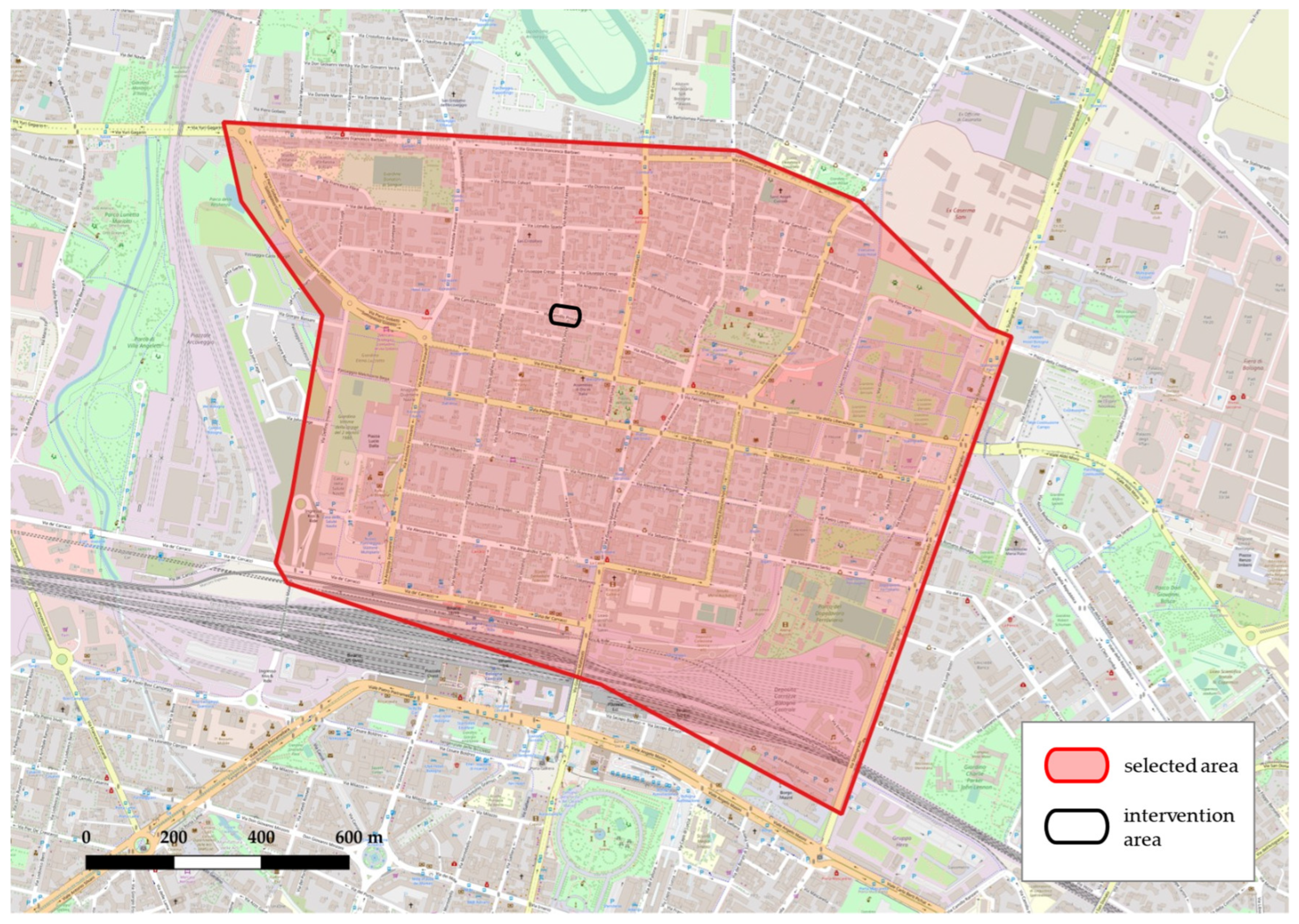
  • area: Bolognina district, Bologna (see Figure 1);
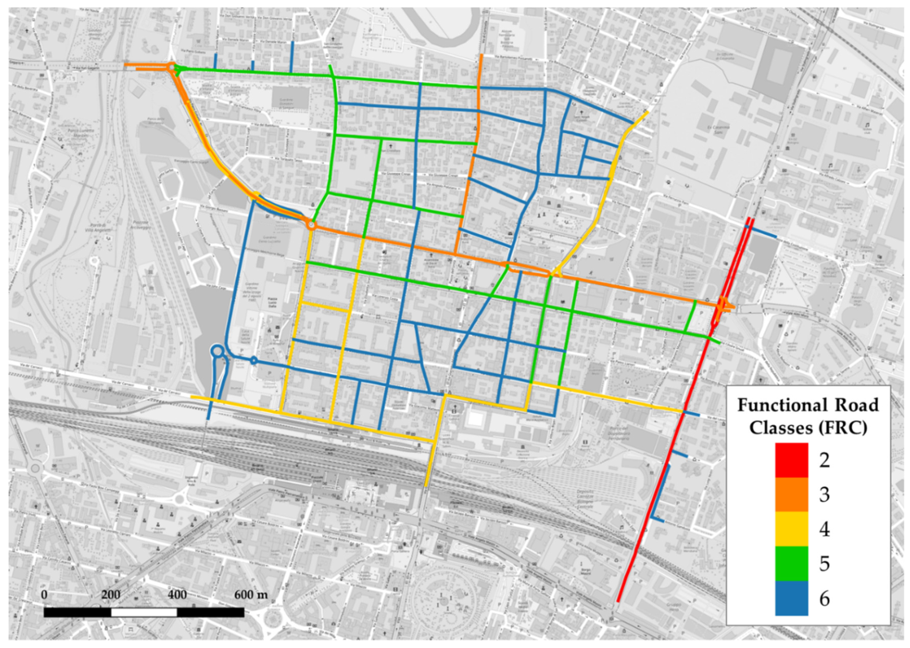
  • FRCs: 1 to 6 (see Figure 2).
Provided sample size is intended as the total number of vehicles registered in the segment through all the days of the sampling period, while each supplied value of speed or travel time is calculated as arithmetical average, harmonic average, median values and standard deviations over each daily slot in the selected date range and specific time fraction.
The choice of periods of time has been made based on the following assumptions:
  • in the months of September and October, schools are open, a fundamental requirement given that the intervention is also expected to impact school-related traffic;
  • a two-month dataset is enough to use as representative for mean traffic values;
  • as the implementation of the temporary square happened in March, ex-post data are collected sufficiently later than the implementation of the temporary square, which is advisable to consider as several pieces of research literature [9,23] encountered unusual congestion in the days straight after the road closure;
  • the same months have been selected for both ex-ante and ex-post scenarios, to avoid issues of seasonality when comparing.
The choice for daily time slots and time fractions has been made in accordance with daily slots and granularity used for video analytics observations on the same intervention and related analyses performed in [6].
Functional Road Classes (whose description is available at: https://support.move.tomtom.com/ts-step-3/, accessed on 1 February 2023) have been subset due to budgetary constraints from 0 to 6; however, this is not an impacting limitation since no motorway segment is included in the selected area and FRC 7 road segments would not improve the dataset and the consequent evaluations with added benefit.

3.2. Methodology

3.2.1. Statistical Trend Analysis

The goal of this first step is to analyse the requested datasets from a macroscopic point of view on the whole network before, and then by clusters identified by proper attributes of road segments in order to detect the magnitude of variations (if there are any) in traffic-related parameters such as sample sizes or speed-related values.
First, to assess significant differences between distinct clusters of available data, a set of Student’s t-tests is performed through statistical tools embedded in Microsoft Excel. In this case, two-tailed paired (or dependent samples) t-tests have been used.
These types of t-tests are used when working with data from different scenarios to compare two datasets and determine if there is a significant difference between them.
More in general, from a more technical perspective, t-tests are based on the rejection of a null hypothesis, formulated at the start of the test; in the case of paired t-tests, in order to ascertain whether there is a substantial difference between the two datasets, the null hypothesis postulates no difference between the means of the two sets of samples. The key result of null hypothesis significance testing is the p-value, standing as the probability of obtaining results as compatible as the observed ones given that the null hypothesis is true. In other words, p-values determine whether any difference between observation sample sets under the null hypothesis is due to randomness, intrinsic in the sampling process, or not. More in detail, after setting a significance level, α, intended as the probability of rejecting the null hypothesis:
  • if  p > α , empirical evidence is not strong enough to reject the initial hypothesis;
  • if  p < α , observed data are statistically significant, so the null hypothesis is rejected.
One of the main assumptions to be made in order to run Student’s t-tests is to assume equal variances between the data samples. A useful rule of thumb often used in statistics states that this assumption works if one variance is up to 3 or 4 times the other, which is valid for every performed t-test (see Table A1, Table A2 and Table A3); a stricter statistical tool to assess the validity of the equal variance assumption is the F-test of equality of variances.
At this early stage of the study, comparisons intend to assess first whether sampled data are a good representation of a real and coherent traffic situation, by evaluating consistent differences between values of speed and sample size recorded for different date ranges (weekdays vs. weekends) and for different FCRs, and then to assess a significant difference between values retrieved for ex-ante and ex-post traffic conditions.
Once data are statistically validated, a set of trend analyses is developed to detect any variations in sample sizes and speed-related values. The main goal is to evaluate the meaning of the differences validated through t-tests between ex-ante and ex-post scenarios, i.e., how much traffic volumes have decreased (or increased) and where on the network, if vehicles travel faster or slower after the intervention, and on which type of streets, by simply comparing corresponding traffic-related parameters. In order to do so, an additional classification of segments is established. According to [5], roads in the network are clustered on the basis of their proximity to the site of intervention. In particular:
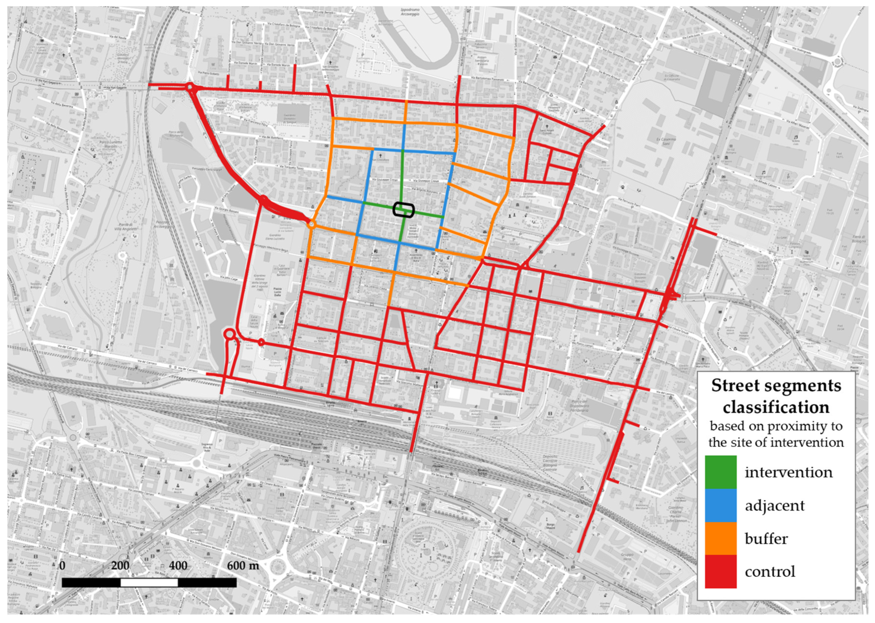
  • the intervention streets are segments directly affected by the modification;
  • adjacent streets are close to the intervention and represent the best alternatives to avoid the site of intervention;
  • streets in the buffer area are no farther than 400 m on road graph distance and so are thought to still be impacted from disturbances caused by the implementation of the temporary school square;
  • all the other roads in the network are classified as control segments, on which global variations of traffic-related parameters will be computed and assumed for the entire network, in order to adjust fluctuations of the other segment clusters and focus on the effects of the intervention.
In Figure 3, road segments in the network are displayed according to this classification.

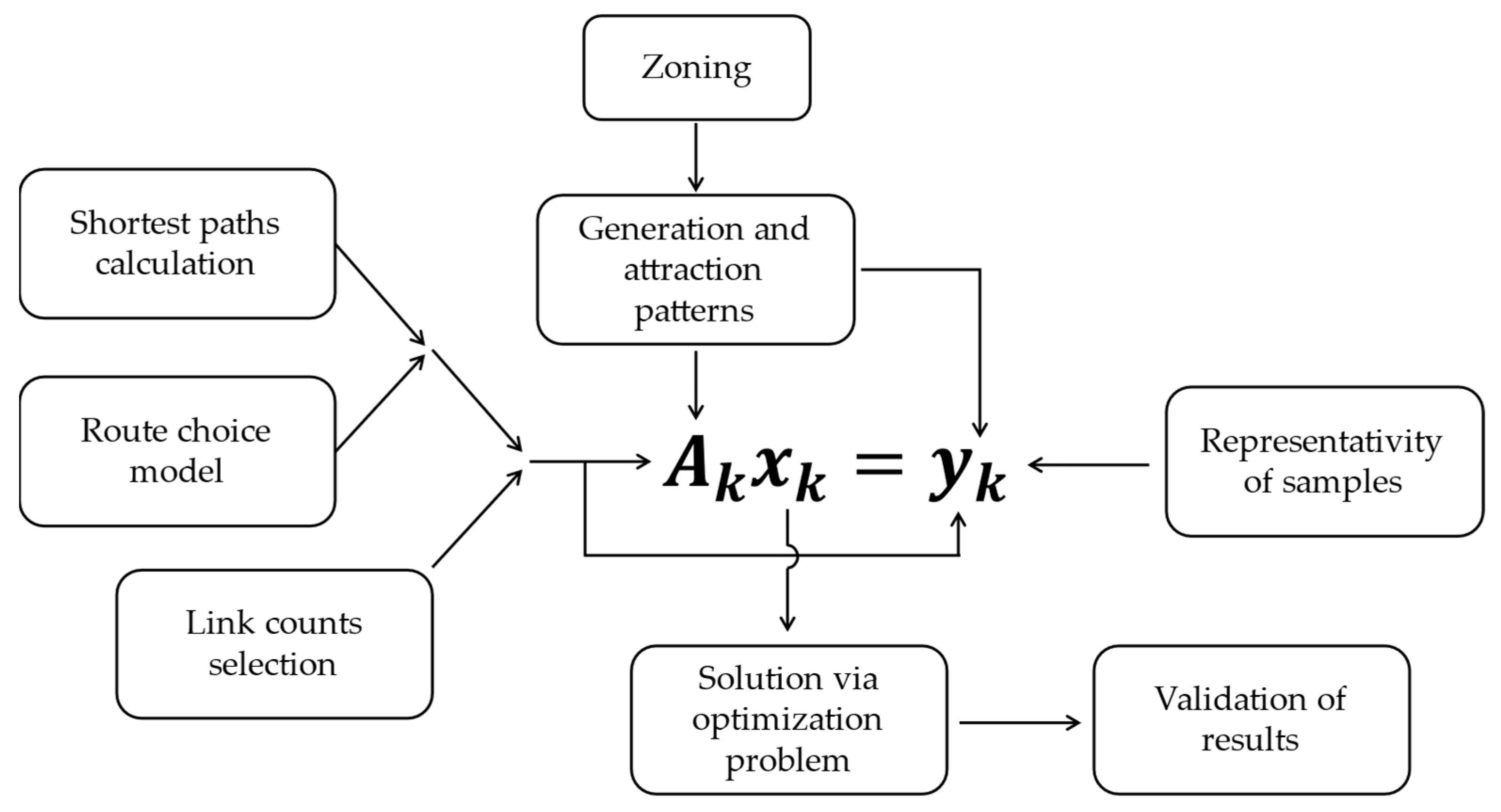
3.2.2. OD Matrices Estimation

The aim of this step is to estimate Origin–Destination matrices which fit the supply patterns extracted from the dataset with the same granularity of available data (one every 15 min). The procedure that will be used is the one proposed in [22].
In this paper, the researchers presented an algorithm that allows one to obtain OD matrices from 3D link supply patterns, intended as values of speed as well as the key figure of transiting vehicles over each time fraction. The algorithm intends to bypass the usual iterative loading of the road network until convergence. It is fundamentally based on the assumptions of cutting off the number of possible shortest paths per OD pair and of attributing a proportional share of the whole pair flow to each path in the previously selected set according to a Path Size Logit (PSL) model using observed travel times as key explanatory variable.
In order to exploit and elaborate available data, a script in R environment has been developed, implementing a version of the proposed algorithm adapted to the case under examination.
As already mentioned before, estimation of OD matrices can be thought of as the inverse process of traffic assignment, being the fourth and last step in the framework of 4-stage traffic models [15].
For an area of study subdivided into n zones, Origin–Destination matrices describing traffic demand on the road network that connects such zones are tables made of  n 2  cells. Under the hypothesis of no intrazonal trips, the problem of OD matrix estimation features  n 2 n  unknowns, provided that zones generate and attract trips at the same time.
Specifically for each time fraction, k, linear equations eligible to solve the problem are identified through traffic counts,  y k m , which can be seen as link flows derived from the combination of the assignment matrix,  A k , and the vector,  x k , containing OD pairs:
A k x k = y k ,
representing a stream of k systems of m linear equations in  n 2 n  unknowns can be either underdetermined, full-rank (in rare cases) or overdetermined; either way, solutions for each time fractions will be extracted solving an optimization problem due to structural inconsistency in the datasets.
In Figure 4, a flow chart summarizing the procedure from raw data to validated OD matrices is displayed:
To ensure representativity of input data—key to decision-making as transport models advising decision makers need to be calibrated over real traffic flows—expansion coefficients,  C e x p , k , have been calculated as a ratio between TomTom sample sizes and traffic counts from video analytics analyses carried out on the same link affected by the intervention [6]. Since the time windows had the same fragmentation, it was possible to extract coefficients per each 15-min fraction, k. At this point, a consistent correlation between the two sets of traffic data could not be established solely for weekend data, so the decision was to exclude such information from the following developments of the research.
An essential requirement for the later application of the procedure is the zoning process. As the network under examination is at neighbourhood scale, origin and destination zones are identified through access and exit streets, i.e., in correspondence with the intersections of the trimming polygon of the selected network and the road graph of the city of Bologna. Such choice of zoning finds itself to be useful for the purpose of micro-simulating the road network once OD matrices are obtained, also avoiding that sample size values on minor local roads could be discarded in the elaboration.
Since the available network extension is much larger than the area which is supposedly affected by the tactical urbanism intervention and in order to ease the OD matrix estimation process by limiting the number of origin and destination zones, a reduction of the segments in the network is performed: via Stalingrado, on the eastern side of the selected area, is removed along with all the eastward afferent segments, as well as the tunnel denominated Asse Nord-Sud and the connection with via de’ Carracci, at the southwestern corner of the network. In Figure 5, removed segments are highlighted in red colour.
The list of origin and destination zones of the edited road network and respective nodes denomination is displayed in Table 1, while in Figure 6 a map highlights the position of origin and destination nodes.
Concerning the first step of a 4-stage transport model, trip generation, a set of input data of generated and attracted trip patterns in each time fraction of 15 min is necessary for the estimation procedure. As availability of sample size data affects each link on the selected network, generation and attraction patterns for OD zones are easily identified with corresponding sample data associated with access/exit segments. These data enforce two fundamental constraints for OD flows:
j x i j k = P i k
i x i j k = A j k
being
  • x i j k  the demand for OD pair i → j of trips departing in time fraction k;
  • P i k  the sum of outbound OD flows from origin node i during time fraction k;
  • A j k  the sum of inbound OD flows to destination node j during time fraction k.
Calculation of shortest paths between origin and destination nodes through a weighted graph is a well-known, computationally demanding challenge in this kind of study. For a portion of urban road network as the one under examination, characterized by a grid layout, calculating all simple paths (i.e., routes without loops and that do not contain the same node more than once), attributing costs according to chosen explanatory variables and then selecting a set containing the most convenient paths, i.e., the ones featuring the minimum costs, can take days for a decent 64-bit calculator, so it is necessary to pursue a faster way.
For each OD pair, a limited set of possible paths is calculated; the chosen algorithm for this step is Yen’s algorithm [24], which computes the first  k ¯  shortest loopless paths for a determined pair of nodes in an oriented graph with non-negative costs attributed to edges. It can employ any effective algorithm for the calculation of the shortest path, then proceeds to compute  k ¯ 1  best deviations with the same algorithm used beforehand.
The underlying logic of the algorithm is as follows: once the first shortest path is computed, for each node i belonging to this path from the origin node, the best alternative way to the destination node is calculated by previously removing the edge (i, i + 1) from the graph; all alternatives are compared regarding the total cost, and the one featuring the lowest value is selected as the best alternative. The algorithm continues to the next iteration until all  k ¯  shortest paths for the selected OD pair are sorted.
For the case study, the algorithm was implemented in the R environment through the library yenpathy, which basically transposes the algorithm script from C++ language; the shortest path computation algorithm adopted by the function in R is Dijkstra’s.
A sensitivity test has been performed with the aim of assessing the determinedness of equation systems resulted from the procedure, which stated that the most suitable number of possible shortest paths is  k ¯ = 4 , given the extent of the network and the number of origin and destination zones resulted from the zoning process. Such choice of  k ¯  would lead overall to slightly underdetermined problems, optimizing the trade-off between severe underdetermination resulting in inconsistent solutions and dispersion of flow on paths whose route choice proportionality is unrealistic.
To attribute route choice proportionality to each path in the calculated set, a Path Size Logit (PSL) model is used; it consists of a Multinomial Logit with travel time as the key explanatory variable, with the addition of penalties for paths that share segments with others in the same set. The main reason for penalizing paths containing shared links is the consideration that the user tends not to recognize one path as a valid alternative if most of the segments are shared between two different choices.
The following PSL model is assumed [25]:
p i j k n = e ( V n + β P S · ln P S n ) r i j k n P i j k e ( V r + β P S · ln P S r )
with
  • p i j k n  route choice proportional factor of path n;
  • V n = C n = T T n k ;
  • β P S  path size parameter to be estimated;
  • P S n  path size factor of path n.
The disutility function,  V n , expresses how costs negatively affect the attractiveness of the choice of path n through explanatory variables, travel time,  T T n k , only in this example. In the event of segments featuring null travel time for time fraction k, indicating that no vehicle has been recorded on the segment, the algorithm automatically converts the attribute value for travel time into 1000 min to exclude such segments from the computation of convenient routes. Lacking useful data for calibration (usually provided by interviews),  β P S  is assumed equal to 1, according to the formulation of the Logit model in the proposed algorithm by [22]. Path sizes are calculated through the original formulation proposed by Ben-Akiva et al. [26]:
P S n = a r i j k n L a L n 1 r i j k n P i j k δ a n
with
  • L a  is the length of link  a ;
  • L n  is the length of path  n ;
  • δ a n  is an integer variable expressing the link-path incidence, i.e., the number of paths in the set which link a features.
It follows that path flows are directly related to OD flows by each proportionality factor:
x i j k n = p i j k n x i j k               i , j , k ; n = 1   N i j k *
Once production and attraction patterns are determined and path sets together with relative choice proportionality are assumed as described beforehand, an additional and essential constraint on OD flows is provided by link traffic counts,  y ~ k = C e x p , k y k , previously increased by the expansion coefficients calculated earlier, which represent the main piece of information for traffic demand.
A link traffic count provides information on OD pairs in the form of these equations:
y k a ~ = r i j k n P k a x i j k n = r i j k n P k a p i j k n x i j k
saying that the expanded traffic count on link  a  in time fraction k is the sum of the path flows,  x i j k n , corresponding to all the paths contained in the set  P k a = r i j k n   |   a   r i j k n .
If the whole set of traffic counts were to be used, the linear system for the determination of OD pairs for each time fraction, k, would feature Equations (2), (3) and (7):
x i 1 k + + x i j k + = P i k x 1 j k + + x i j k + = A j k p 11 k n x 11 k + + p i j k n x i j k + = y k a ~
However, not every configuration of traffic counts can lead to a satisfying solution of the OD estimation problem. For instance, in (8) coefficient matrix  A k  is surely a singular matrix because of dependence among link traffic counts. Indeed, traffic counting suffers from two fundamental problems [27,28]:
  • data inconsistency
    Traffic counts are affected from multiple errors caused by intrinsic flaws in the measurement procedure, leading to inconsistent flows attributed to each link; this means that even if the equation system is full rank, there might be no matrix able to satisfy each value of the observed flow vector; it is thus necessary to consider a vector of errors affecting the set of observed flows.
  • data dependence
    Traffic is modelled over the road network under the hypothesis of flow continuity at nodes, meaning that the difference between inbound and outbound flows must be null; thus, flow on one of the segments related to each node is deductible as a linear combination of the others, leading to linearly dependent equations which would not bring any additional information.
Usually, traffic count campaigns with limited availability of sensors consider such problems and outline a configuration of counting spots, which leads to an independent dataset. As, for the case under examination, link counts are available for each segment for each time fractions in the daily time slots, a criterion for selecting a limited number of independent equations must be assumed.
Yang et al. [29] proposed four basic rules for the selection of optimal locations for link counters:
  • OD pair coverage: a minimum share of demand flow per OD pair should be observed;
  • Maximum flow fraction: for each OD pair, the link with the greatest demand flow fraction between the pair should be observed;
  • Maximum coverage: in the case of limitations of the number of available counters, the greatest number possible of OD pairs is to be observed;
  • Link independence: traffic counts should not be linearly dependent.
On the basis of such rules, localization methods for traffic counters are developed. Most methods presented in the literature proceed from the assumption that a prior OD matrix is available so, by assigning this particular matrix to the network, it is possible to obtain information over used paths between OD pairs and link flows, which constitute input data for localization methods.
In this case, no prior matrix is available; however, information on paths is in fact available because of the formulated assumptions (implications of such premises on the accuracy of the results will be discussed later), so the same methods could be applied to the current case.
The proposed method works as follows:
  • Equations (2) and (3) are chosen as first equations of the linear system, being “privileged” traffic counts providing information of production and attraction patterns, though it should be noted that one equation must be discarded because it is a linear combination of all the others in the set;
  • for each link in the network, excluding access/exit segments, which have already been considered in the previous step, it is computed how many OD pairs have at least one path transiting through the link itself;
  • starting from the link with the highest number of transiting ODs, the corresponding matrix row is added, and a rank check is performed; if the rank of the matrix at this step is lower than the rank of the matrix with the added row, the row is declared linearly independent and the corresponding equation is definitely added to the solving equation system.
The procedure is repeated for all the available traffic counts which, in the current time fraction, have recorded a value greater than 0; all discarded rows that are linearly dependent are placed in a separate container, which will be used to validate resulting OD pair flows once calculated.
In summary, this algorithm seeks to represent as many OD pairs as possible while ensuring that no redundant information is considered, solving the issue of data dependence. Of course, the number of considered possible shortest paths is relevant to the determinedness of the resulting equation system: by increasing the number  k ¯  of considered paths between OD pairs, flows would be dispersed over unrealistically convenient routes, so the benefit of handling more determined equation systems allegedly leading to more consistent solutions would be counterproductive, if not detrimental to the accuracy of final outcomes.
Once link traffic counts are selected, a system of linear equations is obtained for each time fraction k:
A k x k = y ~ k ,
in which  A k x k  represent the vector of estimated link flows and  y ^ k  and  y ~ k  stands for the vector of observed flows multiplied by the corresponding expansion coefficient; in order to avoid meaningless solutions featuring negative OD flows, the vector of unknows, consisting of OD flows in time fraction k, has a non-negativity constraint:  x k 0 .
This equation system can be either underdetermined, full-rank or overdetermined, as the coefficient matrix may not be a square matrix. As a result of the choice of  k ¯ , equation systems both from ex-ante and ex-post situations are slightly underdetermined, with a few cases of full-rank condition.
Nevertheless, the problem raised before about data inconsistency is yet to be confronted. Assumptions on paths and route choice also affect the accuracy of the solution.
To address this issue, it is necessary to consider a vector of errors summarizing measurement errors affecting observed flows, assumption errors and flaws introduced with the proposed model:
A k x k = y ~ k + ε k ,
With the introduction of vector  ε k , independently from the determinedness of each linear system, the solution has to be searched through solving an optimization problem: the objective function  Z x  (11) to be minimized is the norm of vector of errors, which from (10) corresponds to the difference vector between estimated flows and observed flows:
Z x k = ε k 2 = A k x k y ~ k 2 = y ^ k y ~ k 2 .
To solve this optimization problem, the nonlinear Generalized Reduced Gradient (GRG) embedded in the Excel plugin Solve is employed, consisting of an iterative algorithm which calculates at each step the gradient of the objective function, and is therefore suitable for nonlinear “smooth” problems, featuring functions represented by regular hyper surfaces with continuous gradients.
As it needs a first trial solution as a starting point, it could be tricked into recognizing local optima as global solutions. In order to partially overcome this limitation, it is possible to select from Solve plugin settings the option Multistart, which reduces the risk of running into solutions situated in local optima by repeating the procedure starting from different trail solutions, but obviously increasing computational time.
To validate the process of extraction of OD pair flows, linear regressions of considered and discarded link flows between estimations and observations are performed. The aim of this step is to assess the level of correlation between the two sets of link flows, in order to evaluate the accuracy of the determination of OD flows.
The key parameter to be used is the coefficient of determination,  R 2  (R-squared); it is the proportion of how common variance between independent and dependent variables is, so it is used in regression models to evaluate how much of the variance of one variable is explained in the other variable’s variance. High values ( R 2 > 0.7 ) mean good quality correlations; low ones ( R 2 < 0.3 ) show that the two sets are not well correlated.
Correlation coefficient r often overestimates relationship between variables, especially when employed samples are not numerous, while the coefficient of determination tends to be more accurate. Furthermore,  R 2  is usually well defined no matter the nature of the independent variable, if random or fixed.
In case  R 2  drops under the threshold of 0.7, Theil’s inequality coefficient, U, will be computed; although primarily used to evaluate economic inequality, it was proposed by Toledo et al. [30] to statistically validate traffic simulation models. A useful property of this coefficient is that it can overcome the effect of outliers [31], as opposed to usually adopted RMS estimators. U is calculated as follows:
U = 1 n i = 1 n y ^ i y ~ i 2 1 n i = 1 n y ^ i 2 + 1 n i = 1 n y ~ i 2
with
  • n being the number of elements in both the observed and estimated data;
  • y ^ i  the estimations;
  • y ~ i  the observations.
U is bounded between the values of 0 and 1; U = 0 means that measurements and estimations fit perfectly and U = 1 depicts an unacceptable fit. Predicted series featuring U > 0.2 should be disregarded because of their inaccurate character [31].
Theil’s inequality coefficient can be decomposed into three proportions: UM (bias), US (variance) and UC (covariance). In particular, UM gives information about the systematic error, US tells how well the variability is replicated by the model while UC informs about the non-systematic error. Because of how they are constructed, the sum of all three proportions must return 1: the indication of a good fit lies in UM and US being as small as they can get (in return, UC should be as close to 1 as possible).

4. Results

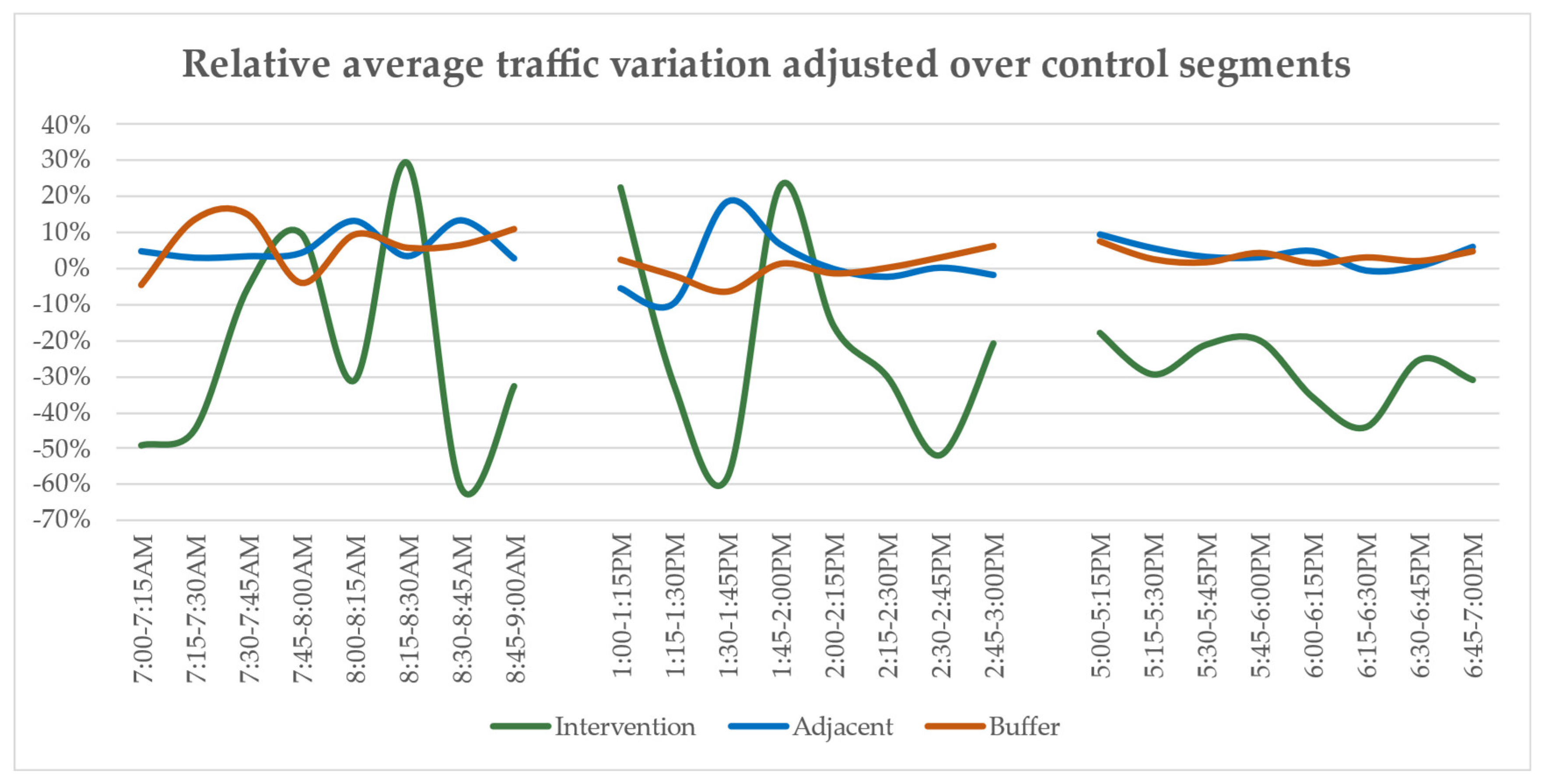
4.1. Statistical Trend Analysis

In the first place, t-tests have been performed comparing datasets by date ranges (weekdays and weekends) and groups of Functional Road Classes (FRC 2–3 and FRC 4–6). The investigated values of the datasets (average speed, sample size and speed 85th percentile) have been condensed in peak time slots through arithmetical average among all the segments belonging to the cluster. Table A1, Table A2 and Table A3 feature mean and standard deviation of both ex-ante and ex-post values, p-values resulted from the statistical test and the difference in means, ΔM.
The null hypothesis stating that the difference in means is zero is rejected in nearly all the tests that have been performed, under the level of probabilistic significance level α = 0.001. A few tests have returned p-values slightly greater than 0.001 but under the threshold value of α = 0.05. The t-test comparing sample sizes in ex-ante and ex-post datasets for FRC 2–3 segments at weekends in the time slot 5:00–7:00 p.m. returned a very high p-value (0.82), so for this specific test the null hypothesis could not be rejected under any reasonable level of probabilistic significance.
On the whole, the available datasets, which have been compared from a statistical significance point of view through t-tests and later by analysing trends, have demonstrated significant differences, so they are worth investigating for mobility pattern variations. However, since from calculating expansion coefficients it was noticed that weekend data could present issues regarding the representativity of real traffic flow data, only values recorded on weekdays have been analysed in the next paragraphs.
In order to assess variations in traffic flow values, the investigated parameter is the sample size adapted to actual values through expansion coefficients to represent real traffic flow, averaged over the entire cluster. For this analysis, road segments have been clustered according to [5] classification regarding the position of the intervention that supposedly triggered the mobility patterns to change.
In Figure 7, average traffic flow on weekdays for intervention streets is displayed:
The intervention street variation trend is characterized by considerable peaks, mostly due to small flows affecting such segments, making it more susceptible to high relative variability. From Figure 7 it is clearly visible that in time slot 5:00–7:00 p.m. traffic flow experienced a reduction of approximately −30%, while the other time slots do not display as clear reduction in flows as the evening slot, being those subject to high fluctuations.
Expectations would suggest that in adjacent or buffer segments traffic flows would also decrease (traffic evaporation), but the data present a different outcome. Of course, traffic levels in a neighbourhood may have changed because of other factors than the temporary school square implementation within a whole year. In order to understand if and how traffic patterns have changed because of the intervention, in Figure 8 the idea is to adjust buffer class variations over control segment fluctuations, with the aim of cancelling the noise sourced from other events that may have affected other zones of the selected road network. Adjusted relative variations have been computed as the difference between the delta values of the buffer classes and the ones for the control class in the same time fraction, k:
i , a , b , k a d j = i , a , b , k c , k
Average indexes of traffic flow variation (see Table 2) consist of mean values per time slot of relative fluctuations for average traffic flows:
From both Figure 8 and Table 2, it is possible to outline findings relative to the impact that the tactical urbanism intervention may have had on the road network:
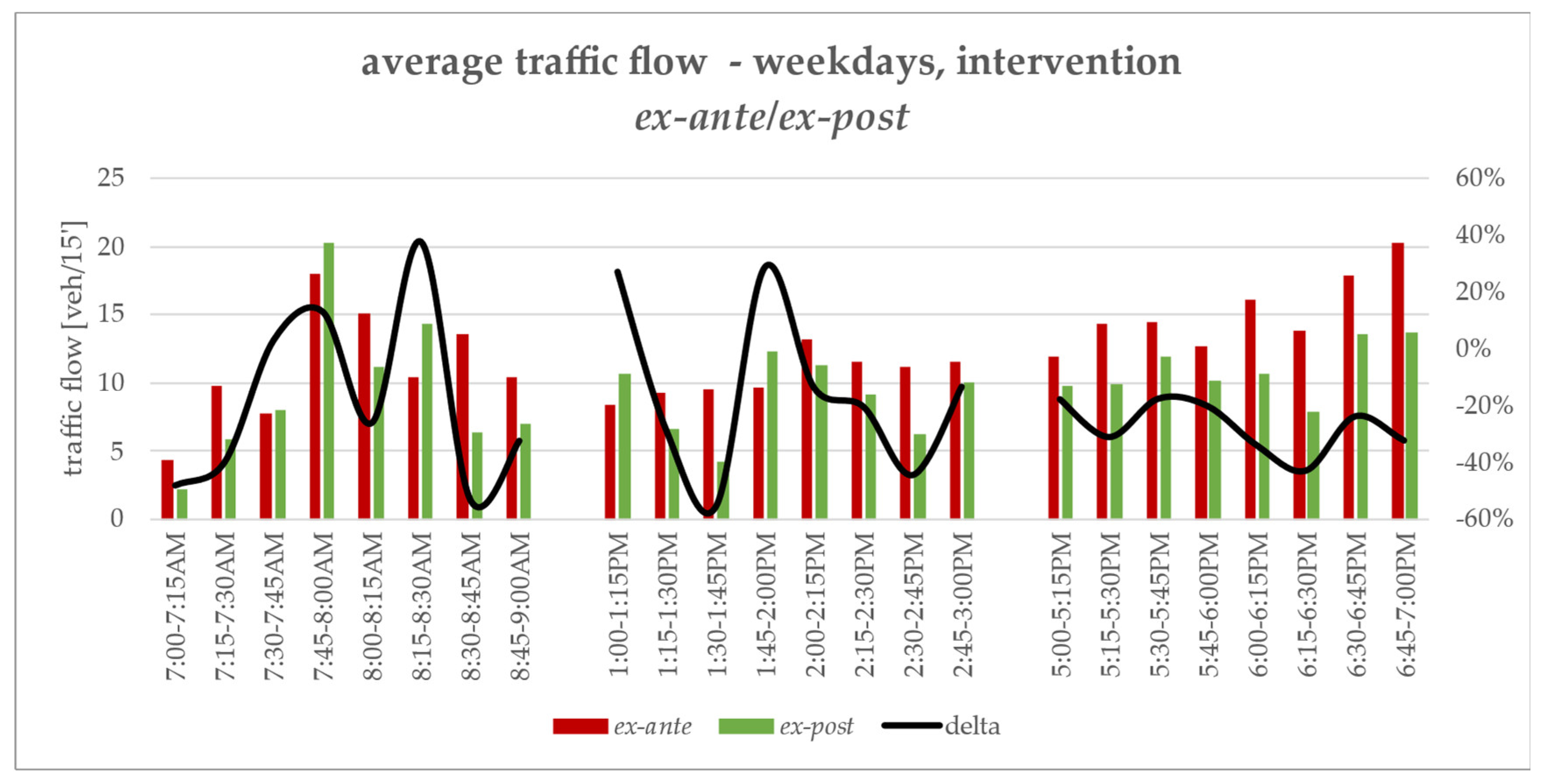
  • the intervention streets, despite presenting considerable peaks due to little flow, so more sensitive to variations, on average faced a consistent reduction, consistent with both the nature and the main purpose of a capacity-limiting, pedestrian-friendly road intervention;
  • segments in the adjacent and buffer zones have recorded, albeit lower both in relative and in absolute terms with respect to intervention segments, a positive relative variation in the matter of traffic flow with respect to the general fluctuations calculated over control segments.
These figures suggest that the implementation of the new temporary school square has moved traffic patterns from the intervention area to alternative paths which deviate from the former most convenient routes using adjacent streets. A further level of interpretation of such data may conclude from available evidence that traffic has disappeared from segments affected by the new implementation, but not from the entire road network (corresponding trend analysis for weekdays on the whole road network is displayed in Figure 9). Thus, the phenomenon of traffic evaporation, encountered in other, more extensive street experiments [5], did not occur here, pointing out that in the case under examination a punctual tactical urbanism could be disruptive to traffic patterns, even if slightly, but did not succeed in diminishing traffic flow in the neighbourhood network.
Sticking to relative fluctuations in traffic flows, network maps have been elaborated through GIS for each time slot, representing percentage changes between ex-ante and ex-post conditions per each segment (see Figure A1, Figure A2 and Figure A3). GIS-generated maps confirm what was noted earlier about the relocation of traffic patterns from segments directly affected by the intervention to adjacent and buffer streets. It is important to underline once again that, in spite of a quite consistent relative reduction in intervention streets, highlighted in the maps through stronger warm colours, surrounding segments have recorded a relatively slight increase in traffic flow, simple because of already considerable traffic flows affecting such segments.
Referring to absolute variation maps elaborated through GIS (see Figure A4, Figure A5 and Figure A6) and supported by global indexes (see Table 2), a clear difference in vehicular patterns emerges, focusing on the surroundings of the new temporary square:
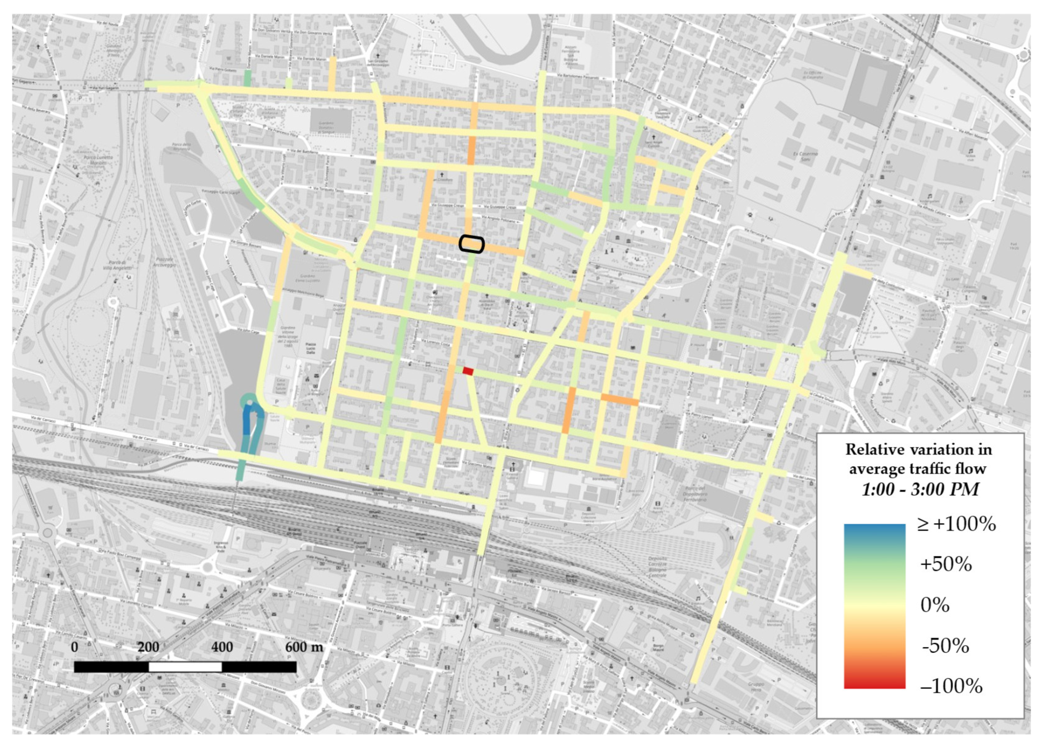
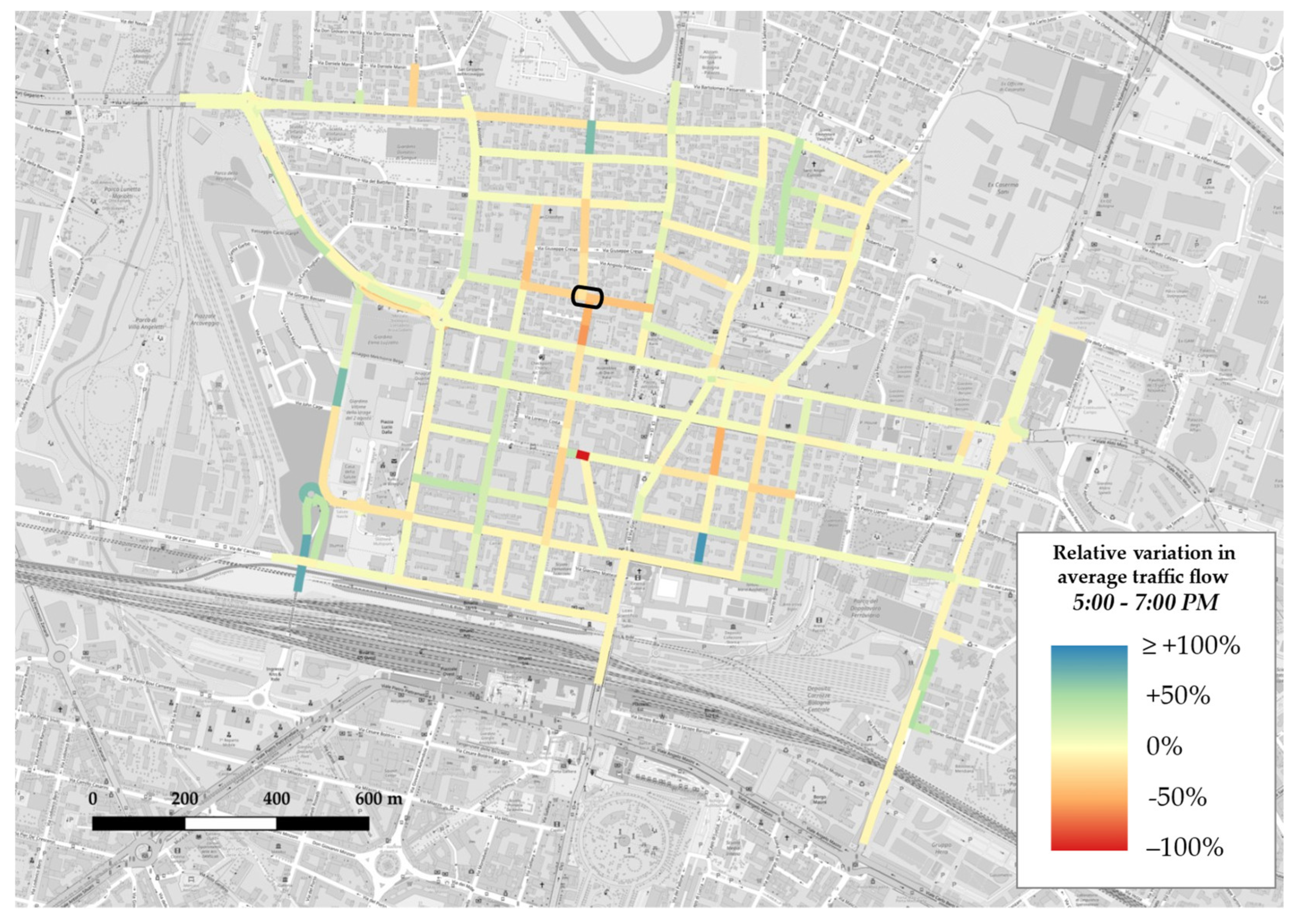
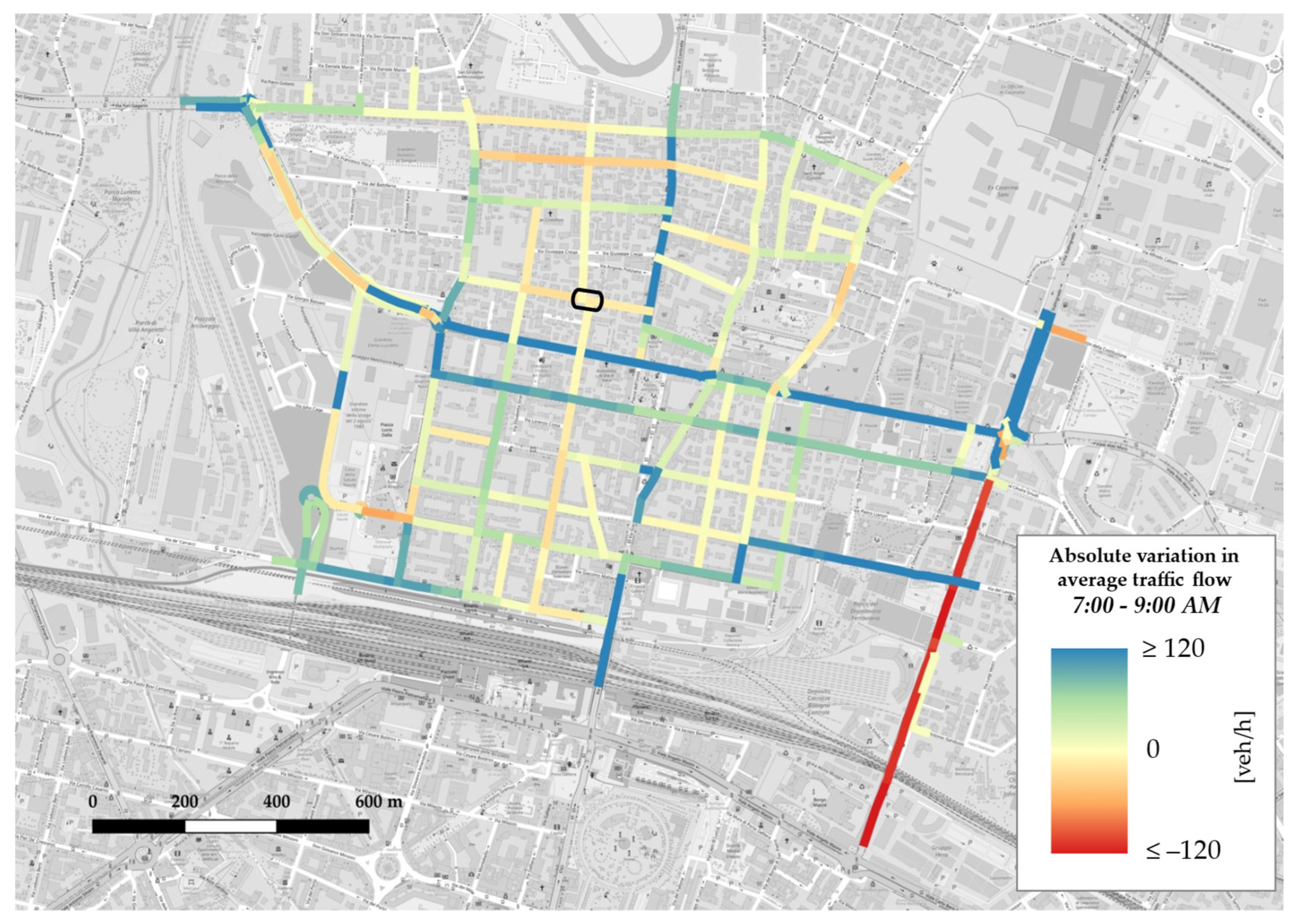
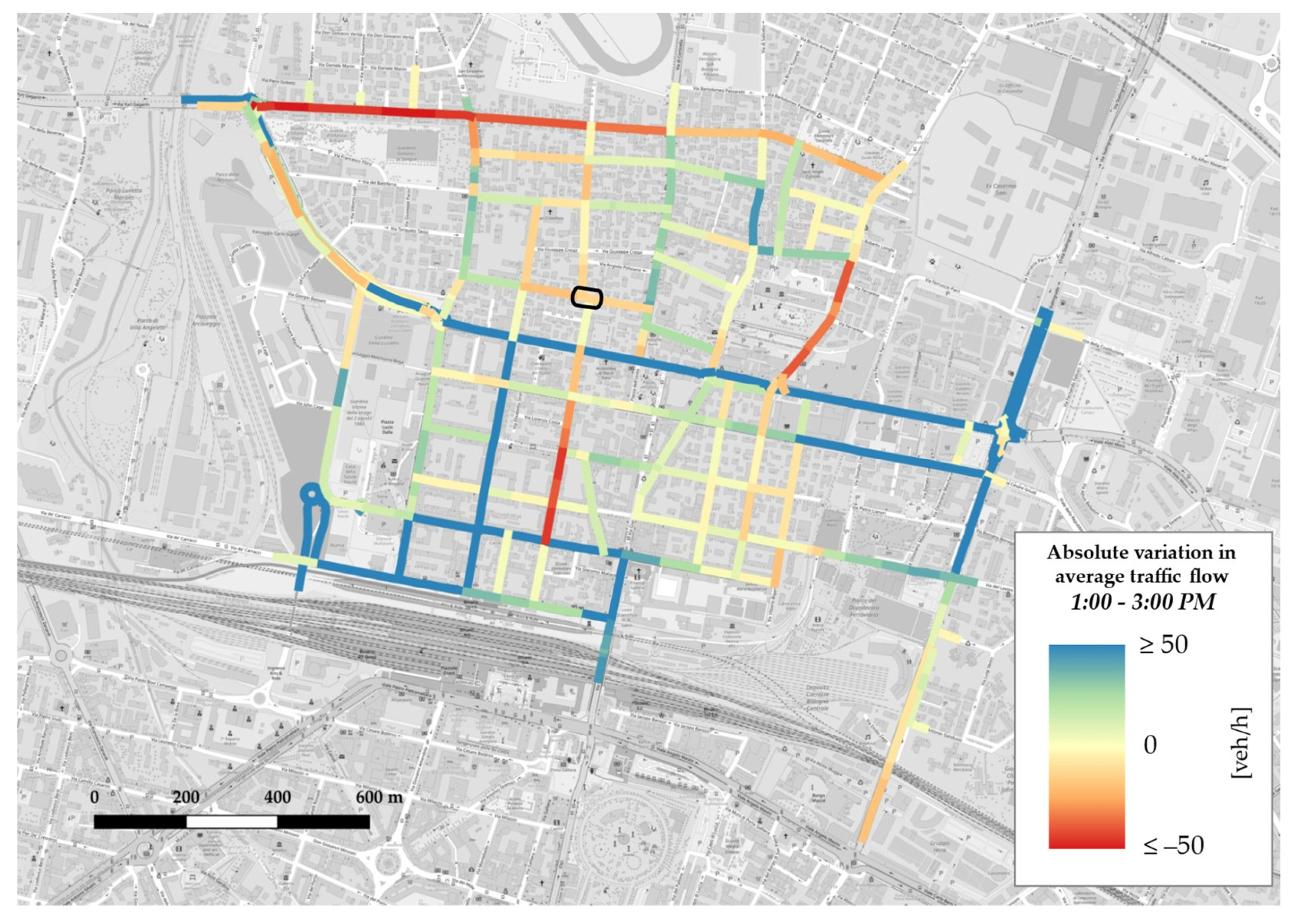
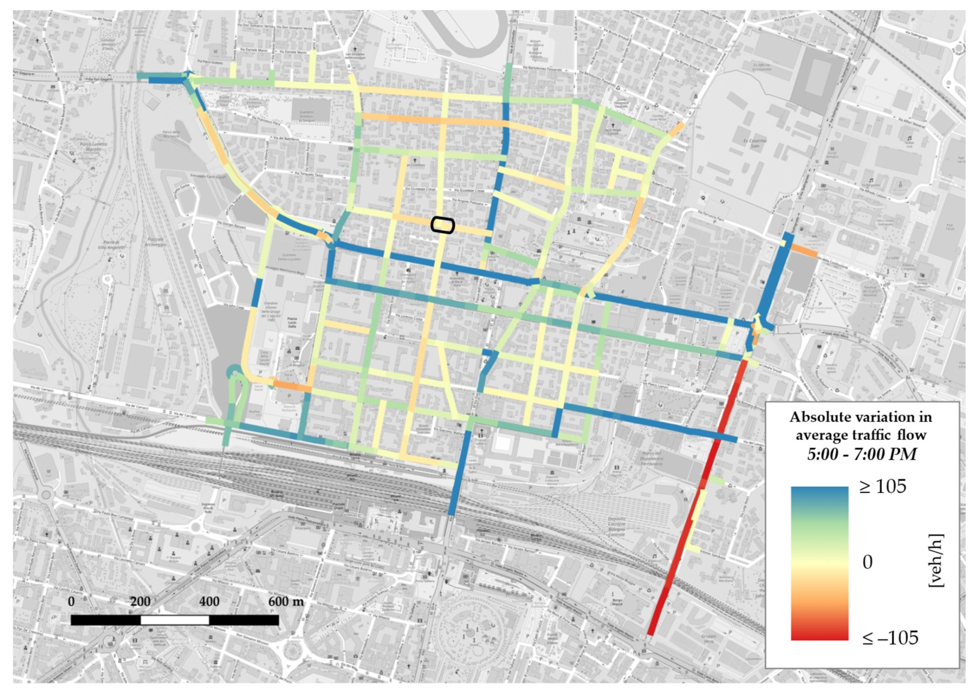
  • intervention segments have recorded a slight negative variation in every addressed time slot;
  • adjoining and neighbouring segments such as the major axis which accesses the neighbourhood from its northern side, or core axes for the east–west through-traffic phenomenon, figuring either in the adjacent or buffer class, have been affected by an appreciable increase in traffic flow.
These considerations stand as a hint of vehicular pattern changes towards a worsening of traffic conditions in the road segments surrounding the intervention area.

4.2. OD Matrices Estimation

Through the process of link counts selection, m, linear equations representing counted segments have been chosen to build non-singular coefficient matrices,  A k , and corresponding vectors of observed traffic flows,  y ~ k .
Following the choice of cutting off the number of possible paths between OD pairs into  k ¯ = 4  most convenient routes in terms of travel times, almost the majority of equation systems used in the algorithm have resulted as slightly underdetermined, with only a couple of exceptions of full-rank conditions. In a few cases, the number of equations has dropped under the threshold of 70; however, this seems not to have affected the results in terms of correlation between estimations and observed flows.
OD matrices for each 15-min fraction, k, have been extracted through the optimization problem, which minimizes the norm of the difference vector between estimated and observed link flows (see Section 3.2.2). Linear regressions between observations and estimations have been established in two separate sets, the first consisting of flows selected to take part in the coefficient matrix, the second containing discarded flows used for the validation of the method. Hence, it is possible to compute coefficients of determination,  R 2 , for each linear regression and to evaluate the accuracy of the estimation process.
From the coefficients of determination calculated (see Figure 10 and Figure 11), correlation between estimated and observed values of link flows once the OD matrix has been elaborated is defined as strong, since  R 2 > 0.7  in every regression for selected flows and almost any correlation for validating the model through discarded flows.
As it is necessary to further inspect regressions whose R-squared is below the acceptance threshold, it is astute to investigate the main factors that could affect the quality of the correlation, and therefore the size of correlation coefficients, r [32]:
(a)
variability in the data;
(b)
matching degree for shapes for distributions;
(c)
nonlinearity;
(d)
outliers;
(e)
sample characteristics;
(f)
measurements errors.
Notwithstanding that (f) is clear and present for every set, it could and surely is affecting correlation quality, the other factors could be investigated to look for the downgrading element.
For each of the “bad performing” correlations, Theil’s inequality coefficient is computed, and later decomposed into its three indicators, which should be able to explain (or at least exclude) which is the problem (Table 3).
From the reported values, regressions featuring lower  R 2 , and for the reason addressed here, present values of U close to the threshold of 0.2. By checking inequality proportion values, it seems that no issue is encountered relative to systematic errors or variability, since the inequality proportions relative to bias and variance stick to small values, certifying the quality of the prediction. Because these statistics do not directly address the effect of outliers, through a qualitative check on linear regression scatterplots (see Figure 12), it is possible to highlight considerable incidences of isolated points (actually streams of points, due to the fragmentation of the underlying road graph).
From Figure 13, some quick but effective remarks both on accuracy of estimated OD matrices and on the general trend of OD flows can be made:
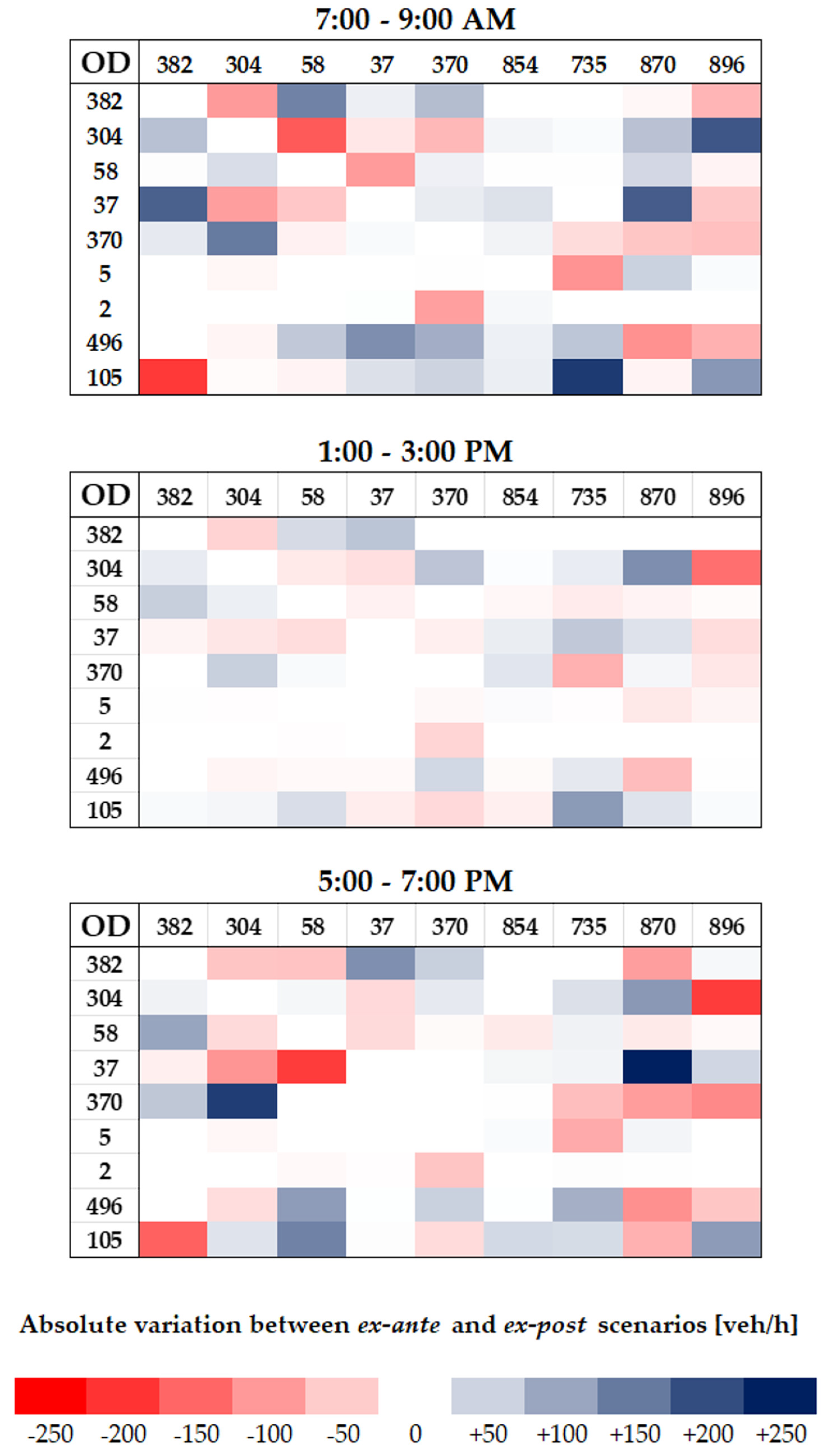
  • in all three matrices, from the lightest shade to the darkest one, blue cells depicting increments are more than red cells, which denote decrements; this is consistent with trend analysis for average traffic flow on weekdays (see Figure 10), which displayed a general rise in each time slot;
  • the darkest colours appear in correspondence with OD pairs whose source and/or sink nodes represent accesses or exits from the network through major axes, in accordance with network absolute variation maps (see Figure A4, Figure A5 and Figure A6), which reported increases on east–west through-traffic routes and main accesses to the neighbourhood from both north and south;
  • time slot 1:00–3:00 p.m. features lighter colours, a sign that absolute variations during lunchtime are lower with respect to the morning and evening slots; this could either suggest a less disrupted pattern behaviour or, more probably, be a consequence of the fact that, as it is not one of the two peak time slots by definition, it reportedly carries less traffic flow, so in absolute terms variations also tend to be less evident.
Further validation of estimated OD matrices will be attainable once the obtained OD demand is fed to micro simulation software that assigns 15-min matrices back to the road network (the process could be done both statically and dynamically) and elaborates network maps displaying estimated flows on each segment to be compared with observations.

5. Discussion

Overall, the applied procedure worked, allowing both to make meaningful considerations about traffic flow variations over the neighbourhood network and to extract reliable OD matrices for each time fraction, k, but there are some limitations that need to be addressed to highlight the implications on the final results.
First, representativity of sampled data is a fundamental step since the main application of the employed procedure is representing real traffic values in order to support decision-making on actual scenarios. To faithfully expand sample sizes, proved expansion coefficients based on actual coverage of accessible sensors should be employed; if not available, it is necessary at least to perform a comparison between flow observations extracted from the set as representative for the sample and traffic counts covering the total flow in the same counting spots and in the same period of the GPS-based sampling process. In any cases, the two datasets to be compared need to be robust estimates of what they represent, so that the expansion coefficient calculation returns reliable multipliers. Nonetheless, as observations systematically contain a considerable number of errors, expansion coefficients will likely amplify such errors. To limit such errors, it is advisable to reach the maximum coverage of road users, even gathering data from different providers, in order to start from a solid database which would be less impacted by the expansion process.
Then, assumptions have been made throughout the procedure in order to smooth the most complicated steps, but this may come at the price of accuracy in the final results.
The choice of cutting off the set of shortest paths to a determined number,  k ¯ , may exclude paths that are significant and actually used by the OD pair demand. Such approximation redistributes discarded path flows on the ones already included in the set, so the final outcome could unrealistically concentrate flows in a few convenient segments according to the assumed cost functions; however, this assumption is needed as the listing of all paths for every considered Origin–Destination pair is computationally way too demanding, and it does not benefit from a practical point of view.
Under the assumption of a common  k ¯  for each OD pair, through sensitivity tests it is possible to choose the most suitable value of such parameter, balancing the credibility of the assumption related to the size of the network under examination (a too large  k ¯  can be counterproductive and also fails to be representative, given the fact that the common user does consider a limited set of paths as alternatives, especially at neighbourhood scale) and the determination of the mathematical problem, in order to obtain consistent outcomes. It could be intelligent to choose an OD-pair-specific  k ¯  to select the appropriate number of possible paths in relation to effectively convenient alternatives for the considered trip.
The Path Size Logit (PSL) model for the calculation of route choice probability only considered experienced travel time as an explanatory variable, though enriched through the path size factor. Other traffic-related variables can be considered, for instance speed limits imposed on segments (with a tight tie in with the 30 km/h zone question, lately widely implemented in most of the road network of the city of Bologna), or the presence of signalized intersections, which may distort the perception of the user on the convenience of the path.
Extraction of 15-min OD matrices overall returned reliable input data for further implementation of simulation models, whose accuracy has been validated through regression parameters. Nevertheless, there are some time fractions that recorded low  R 2  values in the validation via discarded flows. As suggested from evidence in the last section, these weak results in correlation must not be imputed to the determinedness of equation systems (as already said, the number m of equations could not always explain low values for R-squared), but they may find an explication in the proposed criterion of selection of link traffic counts. As outlined previously, the logic was to select segments which could give the richest information by containing as much OD pairs as possible while being independent from already considered equations, in order to avoid the mentioned data dependence issue. The main assumption that led to this proposal is that, even though no prior matrix was available, the two fundamental assumptions regarding path set cut-off and route choice probability provided information about used paths as if a prior matrix were at hand. However, as the underlying logic is based on assumptions, the correlation between actual used paths and predicted ones could have been affected by biases, and so could have the criterion.
However, it is worth understanding why, even if overall OD flows also have fitted discarded link flows after being assigned to the road network, visible inaccuracies have been registered in some time fractions. After considering goodness-of-fit measures such as Theil’s inequality coefficient, U, and its related proportions, which excluded systematic errors as well as the ability to reproduce variability, and by qualitative assessment of linear regression scatterplots, encountered inaccuracies could be explained through the detrimental effect of outliers on such statistical validation tools. In particular, due to the high fragmentation of the road graph provided by TomTom, which negatively affects data inconsistency, if the model assigns an outlying estimation to a road segment, in the linear regression the street is represented by a number of fragments which emphasize the negative outlying effects. To overcome this problem, a possible solution could be the harmonization of the road graph together with segment attributes. It would reduce the number of road segments in the network and ease the layout of the network graph, speeding up calculations of shortest path sets and path choice.
In the end, intrinsic in this method there might be strong biases due to the fact that data have been recorded from vehicles equipped with navigation systems. The construction of sets of paths, as already mentioned, is led once again by the assumption of the user choosing among a selection of best paths. This fits with the ground functioning of navigation systems, as every device informs the user about the best path along with some convenient real-time alternatives together with predicted travel times. This assumption, though, clashes with the nature of systematic trips, which are not guided by any navigation system, but derive from the habits of the systematic traveller. This could be a major limitation, because the algorithm tends to concentrate flows on best paths, discarding actually used segments, and cannot be verified in the absence of ground truth data. This highlights a major limitation of the usage of raw data: the availability of on-board interviews in this case could have been useful to understand if systematic travellers adopted a different behaviour than the one attributed to road users by the overall results.

6. Conclusions

This work was aimed at assessing the effects on private vehicular patterns in the neighbourhood of Bolognina, in the city of Bologna, following the implementation in March 2022 of a temporary square dedicated to young students in via Camillo Procaccini, under the principles of a tactical urbanism approach. It made use of TomTom Floating Car Data collected over the months of September and October 2021 (before the intervention, ex-ante) and 2022 (after the intervention, ex-post), consisting of traffic counts, average speed values and travel times for each segment of the selected road network over three daily time slots and per time fractions of 15 min.
After validating datasets and data clustering through hypothesis tests on statistical significance, trend analyses have shown that traffic flows experienced a slight global increase within a year.
In more detail, under the classification of segments in accordance with graph distance from the intervention site, streets directly affected by the intervention recorded a considerable decrease (−23.87%), with adjacent streets and segments suffering a more contained but positive increase (+3.51% and +3.50%, respectively). This suggests that the phenomenon of traffic evaporation observed in findings related to more widespread implementations of tactical urbanism interventions did not occur at the neighbourhood level in this situation, which exhibited a more impacting traffic flow relocation on alternative paths.
On the whole, the extraction of OD matrices per 15-min time fractions through data-driven procedures returned reliable results, which have been validated through coefficients of determination for regressions between observed and estimated link flows, also thanks to the large availability of data discarded from the equation system construction due to data dependence.
Nonetheless, despite the large number of observations, almost every equation system adopted to extract matrices resulted, even if only slightly, underdetermined; this is because many observations were dependent on the others, due to high fragmentation of the segments in the network (each one with their own supply pattern of traffic-related information), to the grid layout of the road network and to the cut-off of the number of possible paths per OD pair.
Future developments of this work could include:
  • microsimulations of the road network exploiting as demand inputs the extracted OD matrices through the implementation of traditional traffic models, both as further validation of the extracting procedure and as a more thorough assessment of the impact the tactical urbanism intervention had on the private mobility patterns via extraction of traffic-related metrics (queue lengths at intersections, level of service);
  • vehicular network performance-based evaluation of further developments of the design of the temporary school square with the already retrieved input data;
  • a standardization of the trend analyses procedure, aimed at collecting data from other similar road interventions and organizing results based, for instance, on road graph distance or hierarchy of segments on the graph, in order to build a solid reference database designed to advise in the decision-making process;
  • an improvement of the adopted procedure for the estimation of OD matrices through harmonization of the road graph and segment attributes in order to overcome issues such as encountered outliers or considerable data inconsistency;
  • consequently, a standardization of the process aimed at automatizing the extraction of OD flows independently from network size and layout.

Author Contributions

Conceptualization, M.P., G.C. and A.G.; methodology, M.P., G.C. and A.G.; software, M.P., G.C. and L.S.; validation, M.P., G.C., A.G. and L.S.; formal analysis, M.P.; investigation, M.P., G.C. and A.G.; resources, M.P., G.C. and A.G.; data curation, M.P., G.C., L.M. and L.S.; writing—original draft preparation, M.P.; writing—review and editing, M.P., G.C., A.G., L.M. and L.S.; visualization, M.P.; supervision, G.C. and A.G.; project administration, A.G. All authors have read and agreed to the published version of the manuscript.

Funding

This research received no specific grant from any funding agency in the public, commercial, or not-for-profit sectors.

Institutional Review Board Statement

The analysed data were treated according to the GDPR-General Data Protection Regulation (EU, 2016/679).

Informed Consent Statement

Not applicable.

Data Availability Statement

Restrictions apply to the availability of these data. Data was obtained from TomTom MOVE web portal, and data sharing is not applicable to this article.

Conflicts of Interest

The authors declare no conflict of interest.

Appendix A. Results of t-Tests

Table A1. Results of t-tests for average speed values.
Average Speedex-anteex-postp-ValueΔM
MSDMSD
weekdays30.829.7729.749.297.06 × 10−29−1.08 ***7–9 a.m.
31.559.6230.779.172.04 × 10−19−0.77 ***1–3 p.m.
28.139.5927.249.112.78 × 10−18−0.89 ***5–7 p.m.
weekends34.4011.4933.3111.153.07 × 10−12−1.09 ***7–9 a.m.
32.5810.0631.739.676.03 × 10−15−0.86 ***1–3 p.m.
30.559.6529.079.136.80 × 10−25−1.49 ***5–7 p.m.
FRC 2–337.4810.4036.739.792.10 × 10−11−0.76 ***7–9 a.m.
36.619.3836.149.032.55 × 10−7−0.48 ***1–3 p.m.
32.849.2032.189.207.60 × 10−8−0.66 ***5–7 p.m.
FRC 4–630.3810.2529.159.811.53 × 10−23−1.24 ***7–9 a.m.
29.989.3529.018.756.09 × 10−26−0.97 ***1–3 p.m.
27.749.2726.318.544.50 × 10−35−1.43 ***5–7 p.m.
weekdays
FRC 2–3
34.299.6233.649.309.43 × 10−9−0.65 ***7–9 a.m.
35.759.3835.188.901.11 × 10−5−0.57 ***1–3 p.m.
31.019.6330.519.351.06 × 10−3−0.50 **5–7 p.m.
weekdays
FRC 4–6
29.239.4327.968.731.73 × 10−22−1.27 ***7–9 a.m.
29.629.1028.758.583.57 × 10−15−0.87 ***1–3 p.m.
26.818.6025.748.603.59 × 10−16−1.07 ***5–7 p.m.
weekends
FRC 2–3
40.6810.2039.829.291.03 × 10−5−0.86 ***7–9 a.m.
37.489.3237.099.083.69 × 10−3−0.38 **1–3 p.m.
34.689.4333.858.752.04 × 10−5−0.83 ***5–7 p.m.
weekends FRC 4–631.5310.9030.3410.671.22 × 10−8−1.20 ***7–9 a.m.
30.349.5929.278.923.73 × 10−13−1.07 ***1–3 p.m.
28.679.1726.888.454.63 × 10−21−1.79 ***5–7 p.m.
** p < 0.01; *** p <0.001.
Table A2. Results of t-tests for sample size values.
Sample Sizeex-anteex-postp-ValueΔM
MSDMSD
weekdays68.4666.5872.6268.704.60 × 10−554.16 ***7–9 a.m.
61.5260.8964.8864.012.85 × 10−513.36 ***1–3 p.m.
85.0577.5186.1277.189.73 × 10−101.07 ***5–7 p.m.
weekends22.3823.5825.3825.683.41 × 10−863.00 ***7–9 a.m.
51.7857.6856.0760.017.13 × 10−834.28 ***1–3 p.m.
69.9575.7972.3973.655.35 × 10−212.44 ***5–7 p.m.
FRC 2–386.0370.3992.4771.291.29 × 10−626.44 ***7–9 a.m.
108.9170.02116.6771.761.57 × 10−917.76 ***1–3 p.m.
148.8480.84149.8880.843.50 × 10−31.04 **5–7 p.m.
FRC 4–626.8332.3029.1033.884.32 × 10−742.27 ***7–9 a.m.
32.7333.0834.7434.243.64 × 10−622.01 ***1–3 p.m.
44.8444.8746.9245.181.39 × 10−382.09 ***5–7 p.m.
weekdays
FRC 2–3
129.3873.37137.1273.161.20 × 10−287.74 ***7–9 a.m.
115.7468.58123.8670.842.00 × 10−458.12 ***1–3 p.m.
157.9177.75159.8676.073.96 × 10−61.95 ***5–7 p.m.
weekdays
FRC 4–6
40.5739.0943.1040.733.42 × 10−382.52 ***7–9 a.m.
36.7036.0037.8836.854.11 × 10−211.18 ***1–3 p.m.
51.6949.1152.3649.115.36 × 10−50.67 ***5–7 p.m.
weekends
FRC 2–3
42.6827.8047.8228.802.71 × 10−615.14 ***7–9 a.m.
102.0870.95109.4972.122.57 × 10−487.40 ***1–3 p.m.
139.7889.24139.9084.358.24 × 10−10.135–7 p.m.
weekends FRC 4–613.0813.5215.1015.709.00 × 10−392.02 ***7–9 a.m.
28.7629.3931.6131.131.04 × 10−442.85 ***1–3 p.m.
37.9838.5141.4840.211.29 × 10−393.50 ***5–7 p.m.
** p < 0.01; *** p <0.001.
Table A3. Results of t-tests for speed 85th percentile values.
Speed 85th Percentileex-anteex-postp-ValueΔM
MSDMSD
weekdays41.9811.9340.4110.791.14 × 10−14−1.57 ***7–9 a.m.
42.7811.6941.7210.673.40 × 10−9−1.06 ***1–3 p.m.
39.1011.9537.6710.663.21 × 10−12−1.43 ***5–7 p.m.
weekends45.8314.5644.0213.711.71 × 10−12−1.80 ***7–9 a.m.
44.0412.7842.4411.553.45 × 10−11−1.59 ***1–3 p.m.
41.1812.0439.6510.809.39 × 10−10−1.53 ***5–7 p.m.
FRC 2–350.2811.4649.1410.591.66 × 10−11−1.14 ***7–9 a.m.
48.9210.4348.229.752.52 × 10−6−0.70 ***1–3 p.m.
44.5410.1943.9410.197.06 × 10−5−0.60 ***5–7 p.m.
FRC 4–640.9913.2839.0511.976.94 × 10−18−1.94 ***7–9 a.m.
40.8912.2139.2710.577.45 × 10−15−1.62 ***1–3 p.m.
38.1312.0436.2410.155.18 × 10−17−1.89 ***5–7 p.m.
weekdays
FRC 2–3
46.3910.5545.6110.239.51 × 10−11−0.78 ***7–9 a.m.
47.8410.4647.259.735.41 × 10−4−0.59 ***1–3 p.m.
42.6910.9342.1410.441.48 × 10−3−0.55 **5–7 p.m.
weekdays
FRC 4–6
39.9712.0038.0310.192.82 × 10−11−1.94 ***7–9 a.m.
40.4611.5039.1810.123.18 × 10−7−1.28 ***1–3 p.m.
37.4610.1335.6210.131.85 × 10−10−1.84 ***5–7 p.m.
weekends
FRC 2–3
54.1811.0352.679.761.93 × 10−6−1.51 ***7–9 a.m.
50.0010.3049.199.709.22 × 10−4−0.81 ***1–3 p.m.
46.3910.3945.749.638.78 × 10−3−0.65 **5–7 p.m.
weekends FRC 4–642.0014.3940.0713.451.68 × 10−8−1.94 ***7–9 a.m.
41.3112.8839.3511.014.01 × 10−9−1.95 ***1–3 p.m.
38.7912.0136.8610.152.27 × 10−8−1.93 ***5–7 p.m.
** p < 0.01; *** p <0.001.

Appendix B. GIS Maps

Figure A1. Relative variation in average traffic flow—time slot 7:00–9:00 a.m. (Map source: OpenStreetMap).
Sustainability 15 12716 g0a1
Figure A2. Relative variation in average traffic flow—time slot 1:00–3:00 p.m. (Map source: OpenStreetMap).
Sustainability 15 12716 g0a2
Figure A3. Relative variation in average traffic flow—time slot 5:00–7:00 p.m. (Map source: OpenStreetMap).
Sustainability 15 12716 g0a3
Figure A4. Absolute variation in average traffic flow—time slot 7:00–9:00 a.m. (Map source: OpenStreetMap).
Sustainability 15 12716 g0a4
Figure A5. Absolute variation in average traffic flow—time slot 1:00–3:00 p.m. (Map source: OpenStreetMap).
Sustainability 15 12716 g0a5
Figure A6. Absolute variation in average traffic flow—time slot 5:00–7:00 p.m. (Map source: OpenStreetMap).
Sustainability 15 12716 g0a6

References

  1. Cariello, A.; Ferorelli, R.; Rotondo, F. Tactical Urbanism in Italy: From Grassroots to Institutional Tool—Assessing Value of Public Space Experiments. Sustainability 2021, 13, 11482. [Google Scholar] [CrossRef]
  2. Global Design Cities Initiative. How to Implement Street Transformations. A Focus on Pop-Up and Interim Road Safety Projects. Available online: https://globaldesigningcities.org/publication/how-to-implement-street-transformations/ (accessed on 29 June 2023).
  3. United Nations. Transforming Our World: The 2030 Agenda for Sustainable Development; United Nations: New York, NY, USA, 2016. [Google Scholar]
  4. Yassin, H.H. Livable City: An Approach to Pedestrianization through Tactical Urbanism. Alex. Eng. J. 2019, 58, 251–259. [Google Scholar] [CrossRef]
  5. Nello-Deakin, S. Exploring traffic evaporation: Findings from tactical urbanism interventions in Barcelona. Case Stud. Transp. Policy 2022, 10, 2430–2442. [Google Scholar] [CrossRef]
  6. Ceccarelli, G.; Messa, F.; Gorrini, A.; Presicce, D.; Choubassi, R. Deep Learning Analytics for Pre-post Evaluation of Tactical Urbanism Interventions: The Case of Bologna. J. Public Space 2023. submitted. [Google Scholar]
  7. Bertolini, L. From “streets for traffic” to “streets for people”: Can street experiments transform urban mobility? Transp. Rev. 2020, 40, 734–753. [Google Scholar] [CrossRef]
  8. Cairns, S.; Atkins, S.; Goodwin, P.; Bayliss, D. Disappearing traffic? The story so far. Proc. Inst. Civ. Eng. Munic. Eng. 2002, 151, 13–22. [Google Scholar] [CrossRef]
  9. Hunt, J.D.; Brownlee, A.T.; Stefan, K.J. Responses to Centre Street Bridge Closure: Where the “Disappearing” Travelers Went. Transp. Res. Rec. 2002, 1807, 51–58. [Google Scholar] [CrossRef]
  10. Tennøy, A.; Hagen, O.H. Urban main road capacity reduction: Adaptations, effects and consequences. Transp. Res. Part D Transp. Environ. 2021, 96, 102848. [Google Scholar] [CrossRef]
  11. Leduc, G. Road Traffic Data: Collection Methods and Applications. Work. Pap. Energy Transp. Clim. Chang. 2008, 1, 1–55. [Google Scholar]
  12. Necula, E. Analyzing Traffic Patterns on Street Segments Based on GPS Data Using R. Transp. Res. Procedia 2015, 10, 276–285. [Google Scholar] [CrossRef]
  13. Deng, B.; Denman, S.; Zachariadis, V.; Jin, Y. Estimating traffic delays and network speeds from low-frequency GPS taxis traces for urban transport modelling. Eur. J. Transp. Infrastruct. Res. 2015, 15. [Google Scholar] [CrossRef]
  14. D’Andrea, E.; Marcelloni, F. Detection of traffic congestion and incidents from GPS trace analysis. Expert Syst. Appl. 2017, 73, 43–56. [Google Scholar] [CrossRef]
  15. Cascetta, E. Teoria e Metodi Dell’ingegneria dei Sistemi di Trasporto, 2nd ed.; UTET: Torino, Italy, 1998. [Google Scholar]
  16. Bonnel, P.; Fekih, M.; Smoreda, Z. Origin-Destination estimation using mobile network probe data. Transp. Res. Procedia 2018, 32, 69–81. [Google Scholar] [CrossRef]
  17. Fekih, M.; Bellemans, T.; Smoreda, Z.; Bonnel, P.; Furno, A.; Galland, S. A data-driven approach for origin–destination matrix construction from cellular network signalling data: A case study of Lyon region (France). Transportation 2021, 48, 1671–1702. [Google Scholar] [CrossRef]
  18. Croce, A.I.; Musolino, G.; Rindone, C.; Vitetta, A. Estimation of Travel Demand Models with Limited Information: Floating Car Data for Parameters’ Calibration. Sustainability 2021, 13, 8838. [Google Scholar] [CrossRef]
  19. Demissie, M.G.; Kattan, L. Estimation of truck origin-destination flows using GPS data. Transp. Res. Part E Logist. Transp. Rev. 2022, 159, 102621. [Google Scholar] [CrossRef]
  20. Ge, Q.; Fukuda, D. Updating origin–destination matrices with aggregated data of GPS traces. Transp. Res. Part C Emerg. Technol. 2016, 69, 291–312. [Google Scholar] [CrossRef]
  21. Tolouei, R.; Psarras, S.; Prince, R. Origin-destination trip matrix development: Conventional methods versus mobile phone data. Transp. Res. Procedia 2017, 26, 39–52. [Google Scholar] [CrossRef]
  22. Krishnakumari, P.; van Lint, H.; Djukic, T.; Cats, O. A data driven method for OD matrix estimation. Transp. Res. Procedia 2019, 38, 139–159. [Google Scholar] [CrossRef]
  23. Goodwin, P.; Hass-Klau, C.; Cairns, S. Evidence on the Effects of Road Capacity Reductions on Traffic Levels. Traffic Eng. Control 1998, 348–354. [Google Scholar]
  24. Yen, J.Y. Finding the K Shortest Loopless Paths in a Network. Manag. Sci. 1971, 17, 712–716. [Google Scholar] [CrossRef]
  25. Prato, C.G. Route choice modeling: Past, present and future research directions. J. Choice Model. 2009, 2, 65–100. [Google Scholar] [CrossRef]
  26. Ben-Akiva, M.; Bierlaire, M. Discrete Choice Methods and Their Applications to Short Term Travel Decisions. In Handbook of Transportation Science; Kluwer Academic Publishers: New York, NY, USA, 1999; pp. 5–33. [Google Scholar]
  27. Ortúzar, J.; Willumsen, L. Modelling Transport, 4th ed.; Wiley: Bognor Regis, UK, 2011. [Google Scholar]
  28. Espitia Echeverría, E.A. Analisi Dell’influenza Della Localizzazione di Sensori di Rilevamento di Traffico Nell’aggiornamento di Matrici OD—Caso di Studio: Torino. Master’s Thesis, Politecnico di Milano, Milan, Italy, 2018. [Google Scholar]
  29. Yang, H.; Zhou, J. Optimal traffic counting locations for origin–destination matrix estimation. Transp. Res. Part B Methodol. 1998, 32, 109–126. [Google Scholar] [CrossRef]
  30. Toledo, T.; Koutsopoulos, H.N. Statistical Validation of Traffic Simulation Models. Transp. Res. Rec. 2004, 1876, 142–150. [Google Scholar] [CrossRef]
  31. Barceló, J.; Montero, L.; Marqués, L.; Carmona, C. Travel Time Forecasting and Dynamic Origin-Destination Estimation for Freeways Based on Bluetooth Traffic Monitoring. Transp. Res. Rec. 2010, 2175, 19–27. [Google Scholar] [CrossRef]
  32. Goodwin, L.D.; Leech, N.L. Understanding Correlation: Factors That Affect the Size of r. J. Exp. Educ. 2006, 74, 249–266. [Google Scholar] [CrossRef]
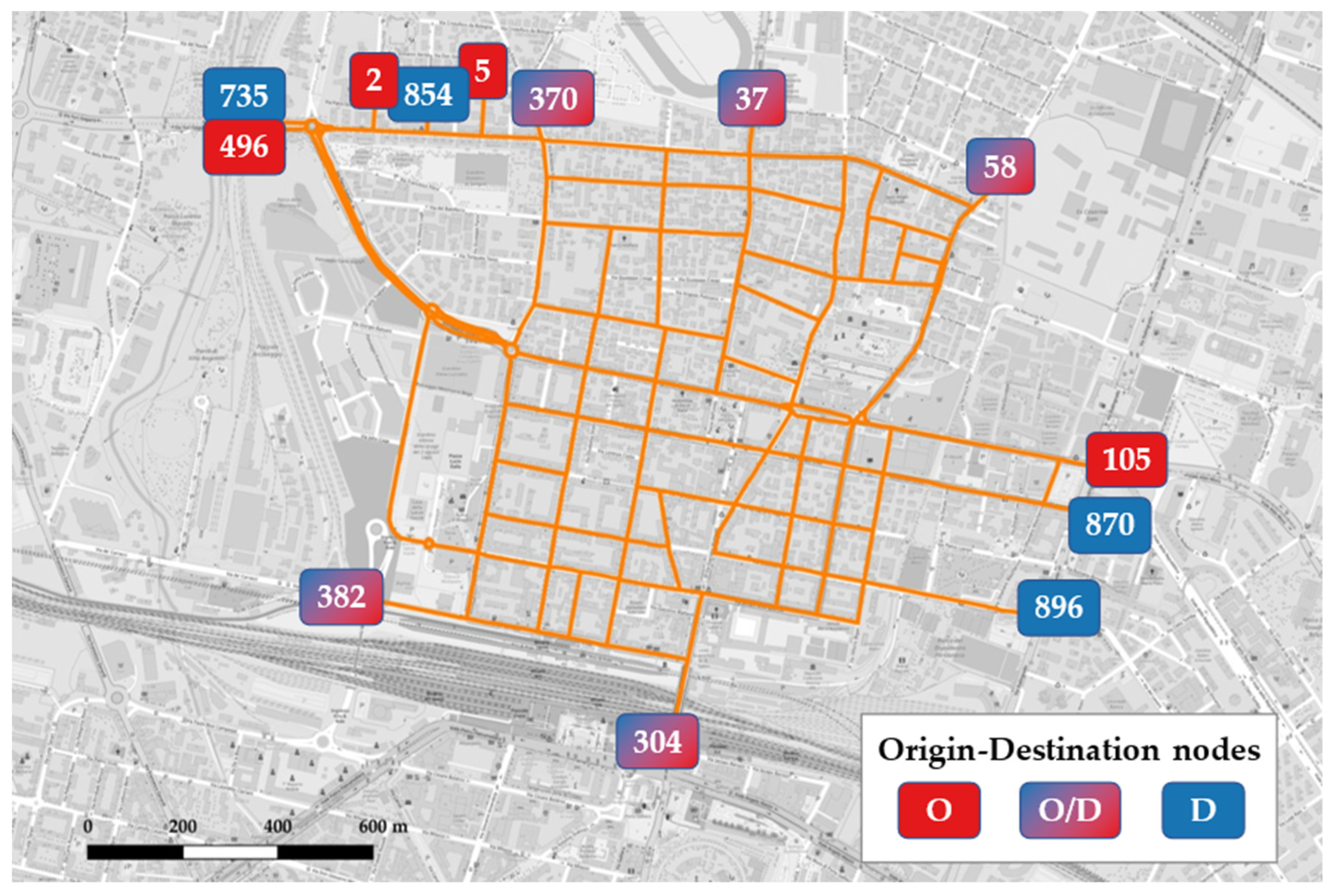
Figure 1. Selected area for TomTom query. (Map source: OpenStreetMap).
Sustainability 15 12716 g001
Figure 2. Functional Road Classes classification. (Map source: OpenStreetMap).
Sustainability 15 12716 g002
Figure 3. Street segment classification based on the proximity to the site of intervention. (Map source: OpenStreetMap).
Sustainability 15 12716 g003
Figure 4. Workflow for OD matrix estimation procedure.
Sustainability 15 12716 g004
Figure 5. Network size reduction. (Map source: OpenStreetMap).
Sustainability 15 12716 g005
Figure 6. Origin–Destination nodes. (Map source: OpenStreetMap).
Sustainability 15 12716 g006
Figure 7. Average traffic flow on weekdays on intervention streets—comparison ex-ante/ex-post.
Sustainability 15 12716 g007
Figure 8. Average traffic relative variation adjusted over control segments.
Sustainability 15 12716 g008
Figure 9. Average traffic flow on weekdays—comparison ex-ante/ex-post.
Sustainability 15 12716 g009
Figure 10. R2 values for ex-ante scenario (green line refers to  R 2 > 0.7 threshold).
Sustainability 15 12716 g010
Figure 11. R2 values for ex-post scenario (green line refers to  R 2 > 0.7  threshold).
Sustainability 15 12716 g011
Figure 12. Linear regression of discarded flows—ex-ante, weekdays, 7:15–7:30 a.m. time fraction.
Sustainability 15 12716 g012
Figure 13. Absolute variation of OD flows between ex-ante and ex-post scenarios.
Sustainability 15 12716 g013
Table 1. Origin–Destination zones (“•” considered zone, “-” not considered zone).
Node IDAccess/Exit SegmentOriginDestination
382Via de’ Carracci
304Via Giacomo Matteotti
58Via Ferrarese
37Via di Corticella
370Via Aristotile Fioravanti
5Via Ezio Cesarini-
854Via Alceste Giovannini-
2Via Daniele Manin-
735Via Yuri Gagarin-
496Via Yuri Gagarin-
105Via della Liberazione-
870Via Donato Creti-
896Via Sebastiano Serlio-
Table 2. Average traffic flow variation relative to control segments.
Buffer Segment Class7:00–9:00 a.m.1:00–3:00 p.m.5:00–7:00 p.m.Average
Intervention−23.11%−20.42%−28.08%−23.87%
Adjacent+5.95%+0.64%+3.94%+3.51%
Buffer+6.57%+0.48%+3.46%+3.50%
Table 3. Theil’s inequality coefficients for low- R 2  regressions.
ex-ante, kex-post, k
2315202423
U0.21100.26990.19130.18430.17680.19970.2091
UM0.00080.01190.01100.00900.00380.00010.0004
US0.00150.05490.00070.00090.00700.00020.0078
UC0.99770.93320.98830.99010.98920.99970.9918
Disclaimer/Publisher’s Note: The statements, opinions and data contained in all publications are solely those of the individual author(s) and contributor(s) and not of MDPI and/or the editor(s). MDPI and/or the editor(s) disclaim responsibility for any injury to people or property resulting from any ideas, methods, instructions or products referred to in the content.

