

Assessing the Chlorophyll-a Retrieval Capabilities of Sentinel 3A OLCI Images for the Monitoring of Coastal Waters in Algoa and Francis Bays, South Africa


Abstract
1. Introduction
- Spectrophotometry involves measuring the amount of light that is absorbed by Chl at a particular wavelength [62].
- High-performance liquid chromatography involves the extraction of Chl molecules from water by absorption, partition, and size exclusion [63].
1.1. Study Area
1.2. Observational Datasets
1.3. Image Pre-Processing and Classification
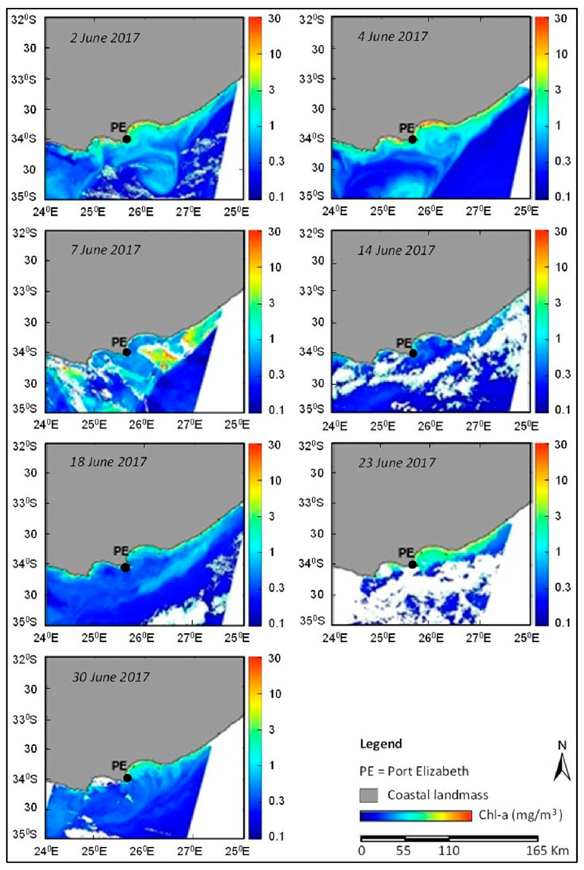
2. Results
3. Discussion
4. Conclusions
Author Contributions
Funding
Institutional Review Board Statement
Informed Consent Statement
Data Availability Statement
Acknowledgments
Conflicts of Interest
References
- Kume, A.; Akitsu, T.; Nasahara, K.N. Why is chlorophyll-b only used in light-harvesting systems? J. Plant Res. 2018, 131, 961–972. [Google Scholar] [CrossRef] [PubMed]
- Fitch, K.; Kemker, C.; Fondriest Environmental, Inc. Algae, Phytoplankton, and Chlorophyll Fundamentals of Environmental Measurements (WWW Document). 2014. Available online: http://www.fondriest.com/environmental-measurements/parameters/water-quality/algaephytoplankton-chlorophyll/ (accessed on 1 January 2016).
- Mishra, S.S.; Mishra, K.N.; Mahananda, M.R. Chlorophyll content studies from inception of leaf buds to leaf-fall stages of teak (tectona grandis) of Kapilash Forest Division, Dhenkanal, Odisha. J. Glob. Biosci. 2013, 2, 26–30. [Google Scholar]
- Mall, L.P.; Billore, S.K.; Misra, C.M. A study on the community chlorophyll content with reference to height and dry weight. Trop. Ecol. 1973, 14, 81–83. [Google Scholar]
- Sheikh, A.Q.; Pandit, A.K.; Ganai, B.A. Seasonal variation in chlorophyll content of some selected plant species of Yousmarg Grassland Ecosystem. Asian J. Plant Sci. Res. 2017, 7, 33–36. [Google Scholar]
- Pilon, L.; Berberoğlu, H.; Kandilian, R. Radiation transfer in photobiological carbon dioxide fixation and fuel production by microalgae. J. Quant. Spectrosc. Radiat. Transf. 2011, 112, 2639–2660. [Google Scholar] [CrossRef]
- Kato, K.; Shinoda, T.; Nagao, R.; Akimoto, S.; Suzuki, T.; Dohmae, N.; Chen, M.; Allakhverdiev, S.I.; Shen, J.-R.; Akita, F.; et al. Structural basis for the adaptation and function of chlorophyll f in photosystem I. Nat. Commun. 2020, 11, 238. [Google Scholar] [CrossRef]
- Chen, M.; Schliep, M.; Willows, R.D.; Cai, Z.-L.; Neilan, B.A.; Scheer, H. A red-shifted chlorophyll. Science 2010, 329, 1318–1319. [Google Scholar] [CrossRef]
- Miyashita, H.; Ikemoto, H.; Kurano, N.; Adachi, K.; Chihara, M.; Miyachi, S. Chlorophyll-d as a major pigment. Nature 1996, 383, 402. [Google Scholar] [CrossRef]
- Strain, H.H.; Cope, B.T., Jr.; McDonald, G.N.; Svec, W.A.; Katz, J.J. Chlorophylls c1 and c2. Phytochemistry 1971, 10, 1109–1114. [Google Scholar] [CrossRef]
- Conant, J.B.; Dietz, E.M.; Bailey, C.F.; Kamerling, S.E. Studies in the chlorophyll series. V. The structure of chlorophyll-a. J. Am. Chem. Soc. 1931, 53, 2382–2393. [Google Scholar] [CrossRef]
- Conant, J.B.; Dietz, E.M.; Werner, T.H. Studies in the chlorophyll series. VIII. The structure of chlorophyll b. J. Am. Chem. Soc. 1931, 53, 4436–4448. [Google Scholar] [CrossRef]
- Gholizadeh, M.H.; Melesse, A.M.; Reddi, L. A comprehensive review on water quality parameters estimation using remote sensing techniques. Sensors 2016, 16, 1298. [Google Scholar] [CrossRef] [PubMed]
- Aminot, A.; Rey, F. Chlorophyll a: Determination by spectroscopic methods. In ICES Techniques in Marine Environmental Sciences; International Council for the Exploration of the Sea: Copenhagen K, Denmark, 2001; pp. 2–16. [Google Scholar] [CrossRef]
- Tang, S.; Liu, F. Remote sensing of phytoplankton decline during the late 1980s and early 1990s in the South China Sea. Int. J. Remote Sens. 2020, 41, 6010–6021. [Google Scholar] [CrossRef]
- Gittings, J.A.; Raitsos, D.E.; Racault, M.F.; Brewin, R.J.; Pradhan, Y.; Sathyendranath, S.; Platt, T. Seasonal phytoplankton blooms in the Gulf of Aden revealed by remote sensing. Remote Sens. Environ. 2017, 189, 56–66. [Google Scholar] [CrossRef]
- Han, L.; Jordan, K.J. Estimating and mapping chlorophyll-a concentration in Pensacola Bay, Florida using Landsat ETM + data. Int. J. Remote Sens. 2005, 26, 5245–5254. [Google Scholar] [CrossRef]
- Available online: https://www.unescwa.org/sites/default/files/inline-files/PPT%20SDG%2014.1.1a_E.pdf (accessed on 15 May 2023).
- Available online: https://wedocs.unep.org/handle/20.500.11822/41997 (accessed on 13 July 2023).
- Available online: https://www.unep.org/explore-topics/sustainable-development-goals/why-do-sustainable-development-goals-matter/goal-14-0 (accessed on 13 July 2023).
- Rombouts, I.; Beaugrand, G.; Artigas, L.F.; Dauvin, J.C.; Gevaert, F.; Goberville, E.; Kopp, D.; Lefebvre, S.; Luczak, C.; Spilmont, N.; et al. Evaluating marine ecosystem health: Case studies of indicators using direct observations and modelling methods. Ecol. Indic. 2013, 24, 353–365. [Google Scholar] [CrossRef]
- Paerl, H.W. Assessing and managing nutrient-enhanced eutrophication in estuarine and coastal waters: Interactive effects of human and climatic perturbations. Ecol. Eng. 2006, 26, 40–54. [Google Scholar] [CrossRef]
- Jeffrey, S.W.; Mantoura, R.F.C. Development of pigment methods for oceanography: SCOR-supported Working Groups and objectives. In Phytoplankton Pigments in Oceanography: Guidelines to Modern Methods; Jeffrey, S.W., Mantoura, R.F.C., Wright, S.W., Eds.; UNESCO: Paris, France, 1997; pp. 19–36. [Google Scholar]
- Bijma, J.; Pörtner, H.-O.; Chris-Yesson, A.D. Climate change and the oceans—What does the future hold? Mar. Pollut. Bull. 2013, 74, 495–505. [Google Scholar] [CrossRef]
- Dasgupta, S.; Ramesh, S.P.; Menas, K. Comparison of global chlorophyll concentrations using MODIS data. Adv. Space Res. 2009, 43, 1090–1100. [Google Scholar] [CrossRef]
- Hynninen, P.H.; Leppäkases, T.S. The Functions of Chlorophylls in Photosynthesis. Physiology and Maintenance V. Available online: http://www.eolss.net/Eolss-sampleAllChapter.aspx (accessed on 23 November 2022).
- Zhang, Z.-C.; Li, Z.-K.; Yin, Y.-C.; Li, Y.; Jia, Y.; Chen, M.; Qiu, B.-S. Widespread occurrence and unexpected diversity of red-shifted chlorophyll producing cyanobacteria in humid subtropical forest ecosystems. Environ. Microbiol. 2019, 21, 1497–1510. [Google Scholar] [CrossRef]
- Chen, M.; Blankenship, R.E. Expanding the solar spectrum used by photosynthesis. Trends Plant Sci. 2011, 16, 427–431. [Google Scholar] [CrossRef] [PubMed]
- Larkum, A.W.D. The evolution of chlorophylls and photosynthesis. In Chlorophylls and Bacteriochlorophylls: Biochemistry, Biophysics, Functions and Applications, Advances in Photosynthesis and Respiration; Grimm, B., Porra, R.J., Rüdiger, W., Scheer, H., Eds.; Springer: New York, NY, USA, 2006; Volume 25, pp. 261–282. [Google Scholar]
- Stomp, M.; Huisman, J.; Stal, L.J.; Matthijs, H.C.P. Colorful niches of phototrophic microorganisms shaped by vibrations of the water molecule. Int. Soc. Microb. Ecol. 2007, 1, 271–282. [Google Scholar] [CrossRef] [PubMed]
- Fondriest Environmental, Inc. Algae, Phytoplankton, and Chlorophyll Fundamentals of Environmental Measurements. 2014. Available online: https://www.fondriest.com/environmental-measurements/parameters/water-quality/algae-phytoplankton-and-chlorophyll (accessed on 24 February 2020).
- Croce, R.; van Amerongen, H. Natural strategies for photosynthetic light harvesting. Nat. Chem. Biol. 2014, 10, 492–501. [Google Scholar] [CrossRef] [PubMed]
- Kirk, J.T.O. Light and Photosynthesis in Aquatic Ecosystems; Cambridge University Press: Cambridge, UK, 2011. [Google Scholar]
- Erickson, Z.K.; Frankenberg, C.; Thompson, D.R.; Thompson, A.F.; Gierach, M. Remote sensing of chlorophyll fluorescence in the ocean using imaging spectrometry: Toward a vertical profile of fluorescence. Geophys. Res. Lett. 2019, 46, 1571–1579. [Google Scholar] [CrossRef]
- Cullen, J.J. The deep chlorophyll maximum: Comparing vertical profiles of chlorophyll-A. Can. J. Fish. Aquat. Sci. 1982, 39, 791–803. [Google Scholar] [CrossRef]
- Boucher, J.; Weathers, K.; Norouzi, H.; Steele, B. Assessing the effectiveness of Landsat 8 chlorophyll a retrieval algorithm for regional freshwater monitoring. Ecol. Appl. 2018, 28, 1044–1054. [Google Scholar] [CrossRef]
- Dai, M.; Zhao, Y.; Chai, F.; Chen, M.; Chen, N.; Chen, Y.; Cheng, D.; Gan, J.; Guan, D.; Hong, Y.; et al. Persistent eutrophication and hypoxia in the coastal ocean. Camb. Prism. Coast. Futur. 2023, 1, e19. [Google Scholar] [CrossRef]
- Mascarenhas, V.; Keck, T. Marine optics and ocean color remote sensing. YOUMARES 8—Oceans across boundaries: Learning from each other. In Proceedings of the 2017 Conference for Young Marine Researchers, Kiel, Germany, 13–15 September 2018; pp. 41–54. [Google Scholar] [CrossRef]
- Anderson, R.C.; Moore, K.S.; Tomlinson, M.C.; Silke, J.; Caroline, K.; Cusack, C.K. Living with harmful algal blooms in a changing world: Strategies for modelling and mitigating their effects in coastal marine ecosystems. In Coastal and Marine Hazards, Risks, and Disasters; Shroder, J.F., Ellis, J.T., Sherman, D.J., Eds.; Elsevier: New York, NY, USA, 2015; pp. 495–561. [Google Scholar] [CrossRef]
- Trainer, V.L.; Pitcher, G.C.; Reguera, B.; Smayda, T.J. The distribution and impacts of harmful algal bloom species in eastern boundary upwelling systems. Prog. Oceanogr. 2010, 85, 33–52. [Google Scholar] [CrossRef]
- Sellner, K.G.; Doucette, G.J.; Kirkpatrick, G.J. Harmful algal blooms: Causes, impacts and detection. J. Ind. Microbiol. Biotechnol. 2003, 30, 383–406. [Google Scholar] [CrossRef]
- Kristiansen, K.D.; Kristensen, E.; Jensen, E.M.H. The influence of water column hypoxia on the behaviour of manganese and iron in Sandy coastal marine sediment. Estuar. Coast. Shelf Sci. 2002, 55, 645–654. [Google Scholar] [CrossRef]
- Grantham, B.A.; Chan, F.; Nielsen, K.J.; Fox, D.S.; Barth, J.A.; Huyer, A.; Lubchenco, J.; Menge, B.A. Upwelling-driven nearshore hypoxia signals ecosystem and oceanographic changes in the Northeast Pacific. Nature 2004, 429, 749–754. [Google Scholar] [CrossRef] [PubMed]
- Naqvi, S.W.A.; Bange, H.W.; Farías, L.; Monteiro, P.M.S.; Scranton, M.I.; Zhang, J. Marine hypoxia/anoxia as a source of CH4 and N2O. Biogeosciences 2010, 7, 2159–2190. [Google Scholar] [CrossRef]
- Limburg, E.; Breitburg, D.; Swaney, D.P.; Jacinto, G. Ocean deoxygenation: A primer. One Earth 2020, 2, 24–29. [Google Scholar] [CrossRef]
- Cain, D.J.; Slomp, C.P. Ocean deoxygenation impacts on microbial processes, biogeochemistry and feedbacks. In Ocean Deoxygenation: Everyone’s Problem-Causes, Impacts, Consequences and Solutions; Lffoley, D., Baxter, J.M., Eds.; IUCN: Gland, Switzerland, 2019; pp. 249–262. [Google Scholar]
- Diaz, R.J.; Rosenberg, R. Spreading dead zones and consequences for marine ecosystems. Science 2008, 321, 926. [Google Scholar] [CrossRef] [PubMed]
- Pitcher, G.C.; Aguirre-Velarde, A.; Breitburg, D.; Cardich, J.; Carstensen, J.; Conley, D.J.; Dewitte, B.; Engel, A.; Espinoza-Morriberón, D.; Flores, G.; et al. System controls of coastal and open ocean oxygen depletion. Prog. Oceanogr. 2021, 197, 102613. [Google Scholar] [CrossRef]
- United Nations Environment Programme (UNEP). Measuring Progress: Water-Related Ecosystems and the SDGs. 2023. Available online: https://wesr.unep.org/measuring-progress/water-related-ecosystems-and-sdgs/sdgs/pdf/DEWA_Measuring_Progress_2023.pdf (accessed on 5 July 2023).
- Lins, R.C.; Martinez, J.-M.; Marques, D.-M.; Cirilo, J.M.; Fragoso, C.R., Jr. Assessment of chlorophyll-a remote sensing algorithms in a productive tropical estuarine-lagoon system. Remote Sens. 2017, 9, 516. [Google Scholar] [CrossRef]
- Cadee, G.C. Book review: Nutrients and eutrophication in estuaries and coastal waters. Aquat. Ecol. 2004, 38, 616–617. [Google Scholar] [CrossRef]
- Cai, W.J.; Hu, X.P.; Huang, W.J.; Murrell, M.C.; Lehrter, J.C.; Lohrenz, S.E.; Chou, W.C.; Zhai, W.D.; Hollibaugh, J.T.; Wang, Y.C.; et al. Acidification of subsurface coastal waters enhanced by eutrophication. Nat. Geosci. 2011, 4, 766–770. [Google Scholar] [CrossRef]
- Rabalais, N.N.; Cai, W.-J.; Carstensen, J.; Conley, D.J.; Fry, B.; Hu, X.; QuiÑOnes-Rivera, Z.; Rosenberg, R.; Slomp, C.P.; Turner, R.E.; et al. Eutrophication-driven deoxygenation in the Coastal Ocean. Oceanography 2014, 27, 172–183. [Google Scholar] [CrossRef]
- Breitburg, D.; Levin, L.A.; Oschlies, A.; Grégoire, M.; Chavez, F.P.; Conley, D.J.; Garçon, V.; Gilbert, D.; Gutiérrez, D.; Isensee, K.; et al. Declining oxygen in the global ocean and coastal waters. Science 2018, 359, eaam7240. [Google Scholar] [CrossRef]
- Beusen, A.; Doelman, J.; Van Beek, L.; Van Puijenbroek, P.J.T.M.; Mogollón, J.M.; Van Grinsven, H.J.M.; Stehfest, E.; Van Vuuren, D.P.; Bouwman, A.F. Exploring River nitrogen and phosphorus loading and export to global coastal waters in the shared socio-economic pathways. Glob. Environ. Chang. 2022, 72, 102426. [Google Scholar] [CrossRef]
- Peñuelas, J.; Sardans, J. The global nitrogen-phosphorus imbalance. Science 2022, 375, 266–267. [Google Scholar] [CrossRef] [PubMed]
- Fernanda, P.; Maciel Haakonsson, S.; Lucía Ponce de León, L.; Bonilla, S.; Pedocchi, F. Challenges for chlorophyll-a remote sensing in a highly variable turbidity estuary, an implementation with sentinel-2. Geocarto Int. 2023, 38, 2160017. [Google Scholar] [CrossRef]
- Pinckney, J.; Papa, R.; Zingmark, R. Comparison of high-performance liquid chromatographic, spectrophotometric, and fluorometric methods for determining chlorophyll-a concentrations in estuarine sediments. J. Microbiol. Methods 1994, 19, 59–66. [Google Scholar] [CrossRef]
- Govindjee, R. Chlorophyll-a fluorescence: A bit of basics and history. In Chlorophyll a Fluorescence, 19; Papageorgiou, G.C., Govindjee, R., Eds.; Springer: Dordrecht, The Netherlands, 2004; pp. 1–41. [Google Scholar] [CrossRef]
- Smith, R.C.; Baker, K.S.; Dustan, P. Fluorometric Techniques for the Measurement of Oceanic Chlorophyll in the Support of Remote Sensing. 1981. Available online: https://escholarship.org/content/qt4k51f7p0/qt4k51f7p0_noSplash_65fc240a49ae6db70e5b0ca4fb6e6f34.pdf (accessed on 15 April 2016).
- Bruce, D.; Vasil’ev, S. Excess light stress: Multiple dissipative processes of excess excitation. In Chlorophyll-a Fluorescence: A Signature of Photosynthesis Advances in Photosynthesis and Respiration 19; Papageorgiou, G.C., Govindjee, Eds.; Springer: Dordrecht, The Netherlands, 2004; pp. 497–523. [Google Scholar]
- Dere, S.; Güneş, T.; Sivac, R. Spectrophotometric determination of Chlorophyll-A, B and total carotenoid contents of some algae species using different solvents. Turk. J. Bot. 1998, 22, 13–18. [Google Scholar]
- Shioi, T.; Fukae, R.; Sasa, T. Chlorophyll analysis by high-performance liquid chromatography. Biochim. Et Biophys. Acta (BBA)—Bioenerg. 1983, 722, 72–79. [Google Scholar] [CrossRef]
- Claustre, H. (Ed.) Bio-optical sensors on argo floats. In Reports of the International Ocean Colour Coordinating Group; IOCCG Report 11; Laboratoire d’Océanographie de Villefranche (LOV-CNRS): Villefranche-sur-mer, France, 2011; p. 89. [Google Scholar]
- Blondeau-Patissier, D.; Gower, J.F.R.; Dekker, A.; Phinn, S.R.; Brando, V.E. A review of ocean color remote sensing methods and statistical techniques for the detection, mapping and analysis of phytoplankton blooms in coastal and open oceans. Prog. Oceanogr. 2014, 123, 123–144. [Google Scholar] [CrossRef]
- Harvey, E.T.; Krause-Jensen, D.; Stæhr, P.A.; Groom, G.B.; Hansen, L.B. Literature review of remote sensing technologies for coastal chlorophyll-a observations and vegetation coverage. In Technical Report from DCE—Danish Centre for Environment and Energy; No. 112; Aarhus University, DCE—Danish Centre for Environment and Energy, 2018; Available online: https://www.researchgate.net/publication/324223737_Literature_review_of_remote_sensing_technologies_for_coastal_chlorophyll-a_observations_and_vegetation_coverage_Technical_Report_from_DCE_-_Danish_Centre_for_Environment_and_Energy_No_112?channel=doi&linkId=5ac6220b0f7e9b1067d5e885&showFulltext=true (accessed on 15 March 2016).
- Dall’Olmo, G.; Gitelson, A.A.; Rundquist, D.C.; Leavitt, B.; Barrow, T.; Holz, J.C. Assessing the potential of SeaWiFS and MODIS for estimating chlorophyll concentration in turbid productive waters using red and near-infrared bands. Remote Sens. Environ. 2005, 96, 176–187. [Google Scholar] [CrossRef]
- Morel, A.; Claustre, H.; Antoine, D.; Gentili, B. Natural variability of bio-optical properties in Case 1 waters: Attenuation and reflectance within the visible and near-UV spectral domains, as observed in South Pacific and Mediterranean waters. Biogeosciences Discuss. 2007, 4, 2147–2178. [Google Scholar] [CrossRef]
- Moore, T.S.; Dowell, M.D.; Bradt, S.; Verdu, A.R. An optical water type framework for selecting and blending retrievals from bio-optical algorithms in lakes and coastal waters. Remote Sens. Environ. 2014, 143, 97–111. [Google Scholar] [CrossRef]
- Gitelson, A.A.; Gurlin, D.; Moses, W.J.; Yacobi, Y.Z. Remote estimation of Chlorophyll-a concentration. In Advances in Environmental Remote Sensing: Sensors, Algorithms, and Applications; CRC Press: Boca Raton, FL, USA, 2011; p. 439. [Google Scholar]
- Matthews, M.W. Bio-optical modeling of phytoplankton chlorophyll-a. In Bio-Optical Modeling and Remote Sensing of Inland Waters; Elsevier: Amsterdam, The Netherlands, 2017; pp. 157–188. [Google Scholar] [CrossRef]
- Ledang, A.B.; Harvey, E.T.; Marty, S. Performance and Applications of Satellite for Water Quality in Norwegian Lakes. Evaluation of MERIS, Sentinel-2 and Sentinel-3 Products. NIVA-Rapport 7443, Norwegian Institute for Water Research, Oslo (Norsk Institutt for Vannforskning). 2019. Available online: https://hdl.handle.net/11250/2655056 (accessed on 24 July 2022).
- Matthews, M.W.; Bernard, S.; Robertson, L.A. A new algorithm for detecting trophic status (chlorophyll-a), cyanobacterial-dominance, surface scums and floating vegetation in coastal and inland waters from MERIS. Remote Sens. Environ. 2012, 124, 637–652. [Google Scholar] [CrossRef]
- Jacobs, Z.; Roberts, M.; Jebri, F.; Srokosz, M.; Kelly, S.; Sauer, W.; Bruggeman, J.; Popova, E. Drivers of productivity on the Agulhas Bank and the importance for marine ecosystems. Deep. Sea Res. 2022, 123, 4447–5067. [Google Scholar] [CrossRef]
- Lutjeharms, W.; Schumann, E.H. Ocean current and temperature structures in Algoa Bay and beyond in November 1986. S. Afr. J. Mar. Sci. 1988, 7, 101–116. [Google Scholar] [CrossRef][Green Version]
- Goschen, W.S.; Bornman, T.G.; Deyzel, S.H.P.; Schumann, E.H. Coastal upwelling on the far eastern Agulhas Bank associated with large meanders in the Agulhas Current. Cont. Shelf Res. 2015, 101, 34–46. [Google Scholar] [CrossRef]
- Jury, M.R. Environmental controls on marine productivity near Cape St. Francis, South Africa. Ocean. Sci. 2019, 15, 1579–1592. [Google Scholar] [CrossRef]
- Malan, N.; Backeberg, B.; Biastoch, A.; Durgadoo, J.V.; Samuelsen, A.; Reason, C.; Hermes, J. Agulhas Current meanders facilitate shelf-slope exchange on the Eastern Agulhas Bank. J. Geophysical. Res. Ocean. 2018, 123, 4446–5067. [Google Scholar] [CrossRef]
- Lutjeharms, J.R.E. The coastal oceans of south-eastern Africa. In The Sea; Robinson, A.R., Brink, K.H., Eds.; Harvard University Press: Cambridge, UK, 2006; pp. 783–834. [Google Scholar]
- Lutjeharms, J.R.E.; Jorge da Silva, A. The Delagoa Bight eddy. Deep. Sea Res. 1988, 35, 619–634. [Google Scholar] [CrossRef]
- Probyn, T.A.; Mitchell-Innes, B.A.; Brown, P.C.; Hutchings, L.; Carter, R.A. A review of primary production and related processes on the Agulhas Bank. S. Afr. J. Mar. Sci. 1994, 90, 166–173. [Google Scholar]
- Hutchings, K.; Porter, S.; Clark, B.M. Marine Specialist Report—Marine Aquaculture Development Zones for Fin Fish Cage Culture in the Eastern Cape: Description of the Affected Environment and Existing Marine Users. 2013. Available online: https://www.daff.gov.za/daffweb3/Branches/Fisheries-Management/Aquaculture-and-Economic-Development/aaquaculture-sustainable-management/Appendix%20B1%20Marine%20Specialist%20Description%20of%20affected%20environment.pdf (accessed on 20 September 2022).
- Roberts, M.J. Chokka squid (Loligo vulgaris reynaudii) abundance linked to changes in South Africa’s Agulhas Bank ecosystem during spawning and the early life cycle. ICES J. Mar. Sci. 2005, 62, 33–55. [Google Scholar] [CrossRef]
- Lombard, A.T.; Strauss, T.; Harris, J.; Sink, K.; Attwood, C.; Hutchings, L. South African national spatial biodiversity assessment 2004. In Marine Component; South African National Biodiversity Institute: Pretoria, South Africa, 2004; Volume 4. [Google Scholar]
- Turpie, J.; Beckley, L.E.; Katua, S.M. Biogeography and the selection of priority areas for conservation of South African coastal fishes. Biol. Conserv. 2000, 92, 59–72. [Google Scholar] [CrossRef]
- Sink, K.J.; Sink, K.; Attwood, C.; Lombard, M.; Grantham, H.; Leslie, R.; Samaai, T.; Kerwath, S.; Majiedt, P.; Fairweather, T.; et al. Systematic Planning to Identify Focus Areas for Offshore Biodiversity Protection in South Africa. Final Report to the Offshore Marine Protected Area Project. 2011. Available online: https://www.cbd.int/doc/meetings/mar/ebsa-sio-01/other/ebsa-sio-01-southafrica-04-en.pdf. (accessed on 23 February 2022).
- Smale, M.J. Distribution and reproduction of the reef fish Petrus rupestris (Pisces: Sparidae) off the coast of South Africa. S. Afr. J. Zool. 1988, 23, 272–287. [Google Scholar] [CrossRef][Green Version]
- Pattrick, P. Assemblage Dynamics of Larval Fishes Associated with Various Shallow Water Nursery Habitats in Algoa Bay, South Africa. Ph.D. Thesis, Nelson Mandela Metropolitan University, Port Elizabeth, South Africa, 2013. Available online: https://core.ac.uk/download/pdf/145048055.pdf (accessed on 18 July 2023).
- Turpie, J.K.; Heydenrych, B.J.; Lamberth, S.J. Economic value of terrestrial and marine biodiversity in the Cape Floristic Region: Implications for defining effective and socially optimal conservation strategies. Biol. Conserv. 2003, 112, 233–251. [Google Scholar] [CrossRef]
- McGrath, M.D.; Horner, C.C.M.; Brouwer, S.L.; Lamberth, S.J.; Mann, B.Q.; Sauer, W.H.H.; Erasmus, C. An economic valuation of the South African linefishery. S. Afr. J. Mar. Sci. 1997, 18, 203–211. [Google Scholar] [CrossRef]
- Schaeffer, B.A.; Loftin, K.A.; Stumpf, R.P.; Werdell, J.P. Agencies collaborate, develop a cyanobacteria assessment network. EOS Earth Space Sci. News 2015, 96. [Google Scholar] [CrossRef]
- Moreira, D.; Pires, J.C. Atmospheric CO2 capture by algae: Negative carbon dioxide emission path. Bio-Resour. Technol. 2016, 215, 371–379. [Google Scholar] [CrossRef]
- Gilerson, A.A.; Gitelson, A.; Zhou, J.; Gurlin, D.; Moses, W.J.; Ioannou, I.; Ahmed, A.A. Algorithms for remote estimation of chlorophyll-a in coastal and inland waters using red and near infrared bands. Opt. Express 2010, 18, 24109–24125. [Google Scholar] [CrossRef]
- Available online: http://coda.eumetsat.int (accessed on 24 February 2014).
- Available online: https://www.saiab.ac.za/about-us.htm (accessed on 13 January 2014).
- Boyd, A.J.; Tromp, B.B.S.; Horstman, D.A. The hydrology off the South African south-western coast between Cape Point and Danger Point in 1975. Afr. J. Mar. Sci. 1985, 3, 145–168. [Google Scholar] [CrossRef]
- Available online: https://step.esa.int/main/download/snap-download/ (accessed on 2 March 2021).
- Available online: https://www.real-statistics.com/statistics-tables/pearsons-correlation-table/ (accessed on 15 August 2022).
- Tóth, V.Z.; Ladányi, M.; Jung, A. Adaptation and validation of a Sentinel-based Chlorophyll-a retrieval software for the Central European freshwater lake, Balaton. PFG J. Photogramm. Remote Sens. Geoinf. Sci. 2021, 89, 335–344. [Google Scholar] [CrossRef]
- Tran, M.D.; Vantrepotte, V.; Loisel, H.; Oliveira, E.N.; Tran, K.T.; Jorge, D.; Mériaux, X.; Paranhos, R. Band ratios combination for estimating Chlorophyll-a from Sentinel-2 and Sentinel-3 in Coastal Waters. Remote Sens. 2023, 15, 1653. [Google Scholar] [CrossRef]
- Le, C.; Hu, C.; Cannizzaro, J.; English, D.; Muller-Karger, F.; Lee, Z. Evaluation of chlorophyll-a remote sensing algorithms for an optically complex estuary. Remote Sens. Environ. 2013, 129, 75–89. [Google Scholar] [CrossRef]
- Gitelson, A.A.; Schalles, J.F.; Hladik, C.M. Remote chlorophyll-a retrieval in turbid, productive estuaries: Chesapeake Bay case study. Remote Sens. Environ. 2007, 109, 464–472. [Google Scholar] [CrossRef]
- Park, K.-E.; Park, J.-E.; Kang, C.-K. Satellite-observed Chlorophyll-a concentration variability in the East Sea (Japan Sea): Seasonal cycle, long-term trend and response to climate index. Front. Mar. Sci. 2022, 9, 807570. [Google Scholar] [CrossRef]
- Yu, Y.; Xing, X.; Liu, H.; Yuan, Y.; Wang, Y.; Chai, F. The variability of chlorophyll-a and its relationship with dynamic factors in the basin of the South China Sea. J. Mar. Syst. 2019, 200, 103230. [Google Scholar] [CrossRef]
- Zhao, N.; Zhang, G.; Zhang, S.; Bai, Y.; Ali, S.; Zhang, J. Temporal-spatial distribution of Chlorophyll-a and impacts of environmental factors in the Bohai Sea and Yellow Sea. IEEE Access 2019, 7, 160947–160960. [Google Scholar] [CrossRef]
- Fernández-Tejedor, M.; Velasco, J.E.; Angelats, E. Accurate estimation of Chlorophyll-a concentration in the coastal areas of the Ebro Delta (NW Mediterranean) using Sentinel-2 and its application in the selection of areas for mussel aquaculture. Remote Sens. 2022, 14, 5235. [Google Scholar] [CrossRef]
- Moutzouris-Sidiris, I.; Topouzelis, K. Assessment of Chlorophyll-a concentration from Sentinel-3 satellite images at the Mediterranean Sea using CMEMS open source in-situ data. Open Geosci. 2021, 13, 85–97. [Google Scholar] [CrossRef]
- Barraza-Moraga, F.; Alcayaga, H.; Pizarro, A.; Félez-Bernal, J.; Urrutia, R. Estimation of Chlorophyll-a concentrations in Lanalhue Lake using Sentinel-2 MSI Satellite Images. Remote Sens. 2022, 14, 5647. [Google Scholar] [CrossRef]
- Binh, N.A.; Hoa, P.V.; Thao, G.T.P.; Duan, H.D.; Thu, P.M. Evaluation of Chlorophyll-a estimation using Sentinel 3 based on various algorithms in southern coastal Vietnam. Int. J. Appl. Earth Obs. Geoinf. 2022, 112, 102951. [Google Scholar] [CrossRef]
- Moses, W.J.; Saprygin, V.; Gerasyuk, V.; Povazhnyy, V.; Berdnikov, S.; Gitelson, A.A. OLCI-based NIR-red models for estimating chlorophyll-a concentration in productive coastal waters—A preliminary evaluation. Environ. Res. Commun. 2019, 1, 011002. [Google Scholar] [CrossRef]
- Cherif, E.K.; Mozeti, P.; Francé, J.; Flander-Putrle, V.; Faganeli-Pucer, J.; Vodopivec, M. Comparison of in-situ Chlorophyll-a time series and Sentinel-3 Ocean and Land Color Instrument data in Slovenian National Waters (Gulf of Trieste, Adriatic Sea). Water 2021, 13, 1903. [Google Scholar] [CrossRef]


| Acquisition Date | Scene ID | % Cloud Cover |
|---|---|---|
| 30 March 2017 | 20170330T064420_20170330T072824_20170330T092717_2644_016_063_MAR_O_NR_002 | 0 |
| 10 May 2017 | 20170510T072056_20170510T080201_20170510T095854_2464_017_263_MAR_O_NR_002 | 5 |
| 2 June 2017 | 20170602T072003_20170602T080429_20170602T100331_2666_018_206_MAR_O_NR_002 | 0 |
| 30 June 2017 | 0170630T065327_20170630T073751_20170630T093231_2664_019_220_MAR_O_NR_002 | 0 |
| 26 July 2017 | 20170726T072040_20170726T080458_20170726T100300_2658_020_206_MAR_O_NR_002 | 5 |
| 8 August 2017 | 20170808T064416_20170808T072831_20170808T092435_2655_021_006_MAR_O_NR_002 | 5 |
| 4 September 2017 | 20170904T064705_20170904T073117_20170904T092051_2652_022_006_MAR_O_NR_002 | 0 |
| 7 October 2017 | 20171007T073608_20171007T082023_20171007T100427_2655_023_092_MAR_O_NR_002 | 5 |
| 31 October 2017 | 20171031T071626_20171031T080043_20171031T094658_2657_024_049_MAR_O_NR_002 | 5 |
| 28 November 2017 | 20171128T065229_20171128T073643_20171128T091641_2654_025_063_MAR_O_NR_002 | 5 |
| 12 December 2017 | 20171212T073029_20171212T081438_20171212T094917_2649_025_263_MAR_O_NR_002 | 10 |
| Acquisition Date | Observed In-Situ Chl-a (mg/m3) Concentrations by Station ID: (P1–P8) | |||||||
|---|---|---|---|---|---|---|---|---|
| P1 | P2 | P3 | P4 | P5 | P6 | P7 | P8 | |
| 29 March 2017 | 10.97 | 30.09 | 4.74 | 13.83 | 12.01 | 25.72 | 9.08 | 9.76 |
| 10 May 2017 | 11.00 | 21.00 | 11.00 | 6.00 | 13.00 | 5.00 | 15.00 | 20.00 |
| 1 June 2017 | 11.06 | 11.10 | 15.45 | 7.00 | 10.50 | 6.76 | 16.79 | 28.74 |
| 30 June 2017 | 16.37 | 19.22 | 11.31 | 10.25 | 9.15 | 12.23 | 10.93 | 12.29 |
| 27 July 2017 | 10.46 | 11.36 | 7.08 | 13.46 | 6.47 | 10.69 | 15.10 | 13.07 |
| 8 August 2017 | 12.98 | 8.79 | 11.81 | 8.63 | 11.33 | 8.35 | 10.93 | 8.84 |
| 5 September 2017 | 13.00 | 8.00 | 12.00 | 8.00 | 8.00 | 6.00 | 12.00 | 8.00 |
| 6 October 2017 | 12.17 | 6.68 | 11.50 | 8.09 | 3.85 | 3.65 | 13.49 | 7.93 |
| 31 October 2017 | 12.33 | 8.25 | 9.86 | 8.55 | 5.42 | 8.63 | 13.29 | 8.44 |
| 28 November 2017 | 12.48 | 9.82 | 8.23 | 9.02 | 6.98 | 13.06 | 7.36 | 12.83 |
| 11 December 2017 | 12.14 | 15.41 | 12.36 | 13.65 | 10.16 | 13.08 | 8.56 | 16.59 |
| Temporal Sequencing of Sentinel 3A and In-Situ Datasets by Station | In-Situ and Sentinel Image-Based Chl-a Concentration Measurements (mg/m3) | ||||
|---|---|---|---|---|---|
| Station ID | Sentinel | In-situ data | In-situ | (NIR-2) | (NIR-3) |
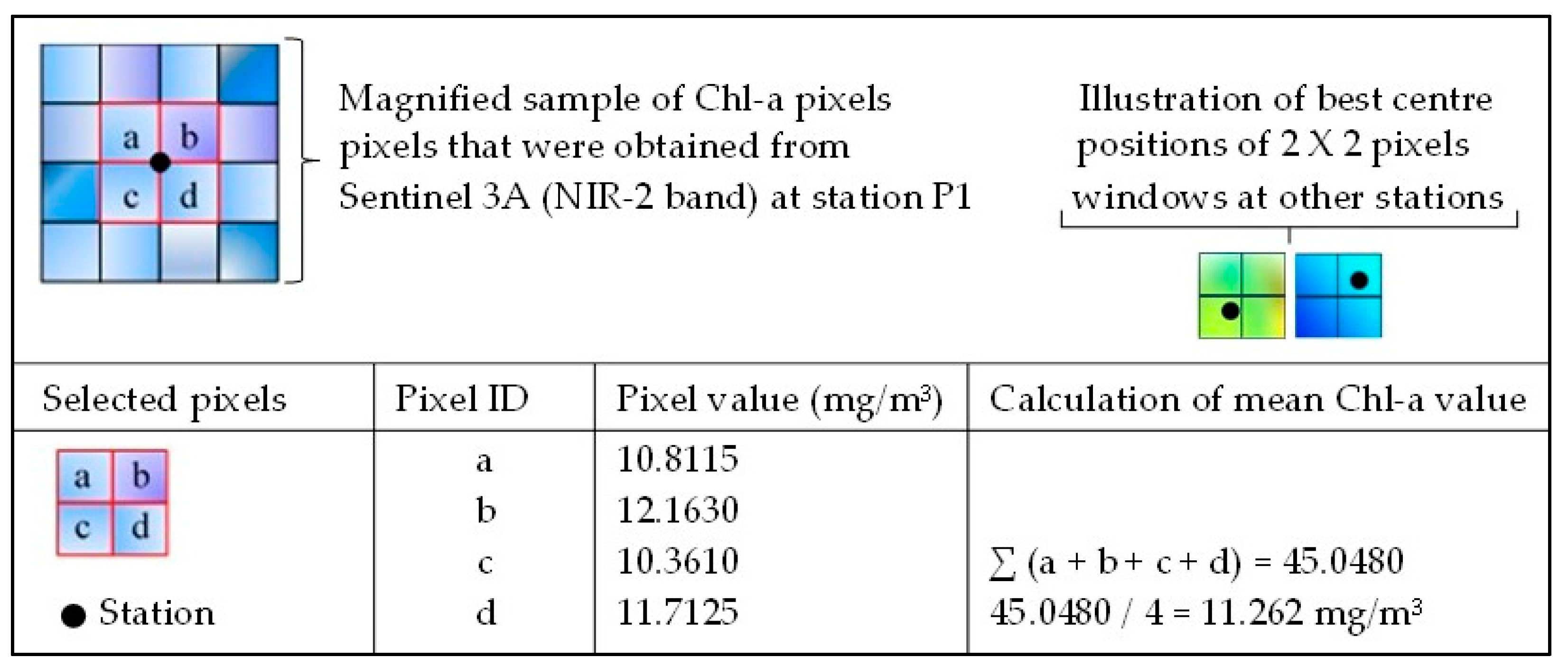
| P1 | 30 March 2017 | 30 March 2017 | 10.97 | * 11.262 | 11.339 |
| 10May 2017 | 10 May 2017 | 11.00 | 11.320 | 11.317 | |
| 2 June 2017 | 4 June 2017 | 11.06 | 11.320 | 11.287 | |
| 30 June 2017 | 30 June 2017 | 16.37 | 11.420 | 11.273 | |
| 26 July 2017 | 26 July 2017 | 10.46 | 11.301 | 11.319 | |
| 8 August 2017 | 8 August 2017 | 12.98 | 11.311 | 11.321 | |
| 4 September 2017 | 4 September 2017 | 13.00 | 11.309 | 11.332 | |
| 6 October 2017 | 7 October 2017 | 12.17 | 11.300 | 11.316 | |
| 31 October 2017 | 31 October 2017 | 12.33 | 11.411 | 11.158 | |
| 28 November 2017 | 28 November 2017 | 12.48 | 11.319 | 11.333 | |
| 11 December 2017 | 12 December 2017 | 12.14 | 11.322 | 11.267 | |
| Mean | - | - | 12.27 | 11.327 | 11.297 |
| St-dev | - | - | 1.611 | 0.047 | 0.052 |
| P-2 | 30 March 2017 | 30 March 2017 | ** 30.09 | 11.262 | 11.405 |
| 10 May 2017 | 10 May 2017 | ** 21.00 | 11.340 | 11.255 | |
| 2 June 2017 | 4 June 2017 | 11.10 | 11.327 | 11.272 | |
| 30 June 2017 | 30 June 2017 | ** 19.22 | 11.250 | 13.908 | |
| 26 July 2017 | 26 July 2017 | ** 11.36 | 11.299 | 11.321 | |
| 8 August 2017 | 8 August 2017 | 8.790 | 11.297 | 11.293 | |
| 4 September 2017 | 4 September 2017 | 8.000 | 11.298 | 11.317 | |
| 6 October 2017 | 7 October 2017 | 6.650 | 11.257 | 12.066 | |
| 31 October 2017 | 31 October 2017 | 8.250 | 11.263 | 11.413 | |
| 28 November 2017 | 28 November 2017 | 9.820 | 11.298 | 11.324 | |
| 11 December 2017 | 12 December 2017 | 15.41 | 11.311 | 11.301 | |
| Mean | - | - | 13.61 | 11.291 | 11.625 |
| St-dev | - | - | 7.201 | 0.030 | 0.791 |
| P-3 | 30 March 2017 | 30 March 2017 | 4.740 | 11.270 | 11.283 |
| 10 May 2017 | 10 May 2017 | 11.00 | 11.345 | 11.248 | |
| 2 June 2017 | 4 June 2017 | 15.45 | 11.326 | 11.295 | |
| 30 June 2017 | 30 June 2017 | 11.31 | 11.298 | 11.305 | |
| 26 July 2017 | 26 July 2017 | 7.080 | 11.301 | 11.320 | |
| 8 August 2017 | 8 August 2017 | 11.81 | 11.299 | 11.317 | |
| 4 September 2017 | 4 September 2017 | 12.00 | 11.301 | 11.320 | |
| 6 October 2017 | 7 October 2017 | 11.50 | 11.255 | 12.286 | |
| 31 October 2017 | 31 October 2017 | 9.860 | 11.249 | 11.251 | |
| 28 November 2017 | 28 November 2017 | 8.230 | 11.305 | 11.308 | |
| 11 December 2017 | 12 December 2017 | 12.36 | 11.358 | 11.228 | |
| Mean | - | - | 10.49 | 11.301 | 11.378 |
| St-dev | - | - | 2.903 | 0.034 | 0.303 |
| P-4 | 30 March 2017 | 30 March 2017 | 13.83 | 11.205 | 10.507 |
| 10 May 2017 | 10 May 2017 | 6.000 | 11.322 | 11.276 | |
| 2 June 2017 | 4 June 2017 | 7.000 | 11.296 | 11.320 | |
| 30 June 2017 | 30 June 2017 | 10.25 | 11.291 | 11.321 | |
| 26 July 2017 | 26 July 2017 | 13.46 | 11.301 | 11.319 | |
| 8 August 2017 | 8 August 2017 | 8.630 | 11.296 | 11.316 | |
| 4 September 2017 | 4 September 2017 | 8.000 | 11.299 | 11.307 | |
| 6 October 2017 | 7 October 2017 | 8.090 | 11.279 | 11.403 | |
| 31 October 2017 | 31 October 2017 | 8.550 | 11.373 | 11.234 | |
| 28 November 2017 | 28 November 2017 | 9.020 | 11.258 | 11.413 | |
| 11 December 2017 | 12 December 2017 | 13.65 | 11.330 | 11.460 | |
| Mean | - | - | 9.680 | 11.295 | 11.261 |
| St-dev | - | - | 2.766 | 0.042 | 0.258 |
| P-5 | 30 March 2017 | 30 March 2017 | 12.01 | 11.320 | 11.342 |
| 10 May 2017 | 10 May 2017 | 13.00 | 11.339 | 11.252 | |
| 2 June 2017 | 4 June 2017 | 10.50 | 11.406 | 11.164 | |
| 30 June 2017 | 30 June 2017 | 9.150 | 11.305 | 11.303 | |
| 26 July 2017 | 26 July 2017 | 6.470 | 11.308 | 11.302 | |
| 8 August 2017 | 8 August 2017 | 11.33 | 11.330 | 11.269 | |
| 4 September 2017 | 4 September 2017 | 8.000 | 11.302 | 11.306 | |
| 6 October 2017 | 7 October 2017 | 3.850 | 11.249 | 11.251 | |
| 31 October 2017 | 31 October 2017 | 5.420 | 11.376 | 11.249 | |
| 28 November 2017 | 28 November 2017 | 6.980 | 11.324 | 11.295 | |
| 11 December 2017 | 12 December 2017 | 10.16 | 11.379 | 11.196 | |
| Mean | - | - | 8.806 | 11.331 | 11.266 |
| St-dev | - | - | 2.907 | 0.044 | 0.052 |
| P-6 | 30 March 2017 | 30 March 2017 | ** 25.72 | 11.251 | 11.146 |
| 10 May 2017 | 10 May 2017 | 5.000 | 11.337 | 11.259 | |
| 2 June 2017 | 4 June 2017 | 6.760 | 11.332 | 11.268 | |
| 30 June 2017 | 30 June 2017 | ** 12.23 | 11.305 | 11.287 | |
| 26 July 2017 | 26 July 2017 | ** 10.69 | 11.816 | 10.489 | |
| 8 August 2017 | 8 August 2017 | 8.350 | 11.322 | 11.276 | |
| 4 September 2017 | 4 September 2017 | 6.000 | 11.301 | 11.315 | |
| 6 October 2017 | 7 October 2017 | 3.650 | 11.249 | 11.251 | |
| 31 October 2017 | 31 October 2017 | 8.630 | 11.249 | 11.251 | |
| 28 November 2017 | 28 November 2017 | ** 13.06 | 11.328 | 11.275 | |
| 11 December 2017 | 12 December 2017 | ** 13.08 | 11.498 | 11.032 | |
| Mean | - | - | 10.288 | 11.363 | 11.168 |
| St-dev | - | - | 6.057 | 0.165 | 0.239 |
| P-7 | 30 March 2017 | 30 March 2017 | 9.05 | 11.300 | 11.309 |
| 10 May 2017 | 10 May 2017 | 15.00 | 11.333 | 11.403 | |
| 2 June 2017 | 4 June 2017 | 16.79 | 11.315 | 11.293 | |
| 30 June 2017 | 30 June 2017 | 10.93 | 11.300 | 11.306 | |
| 26 July 2017 | 26 July 2017 | 15.10 | 11.304 | 11.313 | |
| 8 August 2017 | 8 August 2017 | 10.93 | 11.316 | 11.289 | |
| 4 September 2017 | 4 September 2017 | 12.00 | 11.306 | 11.314 | |
| 6 October 2017 | 7 October 2017 | 13.49 | 11.249 | 11.251 | |
| 31 October 2017 | 31 October 2017 | 13.29 | 11.249 | 11.251 | |
| 28 November 2017 | 28 November 2017 | 7.300 | 11.225 | 10.887 | |
| 11 December 2017 | 12 December 2017 | 8.560 | 11.405 | 11.159 | |
| Mean | - | - | 12.040 | 11.300 | 11.252 |
| St-dev | - | - | 3.006 | 0.048 | 0.135 |
| P-8 | 30 March 2017 | 30 March 2017 | 9.760 | 11.247 | 11.526 |
| 10 May 2017 | 10 May 2017 | ** 20.00 | 11.323 | 11.277 | |
| 2 June 2017 | 4 June 2017 | ** 28.74 | 11.304 | 11.295 | |
| 30 June 2017 | 30 June 2017 | 12.29 | 11.288 | 11.313 | |
| 26 July 2017 | 26 July 2017 | 13.07 | 11.299 | 11.330 | |
| 8 August 2017 | 8 August 2017 | 8.940 | 11.309 | 11.315 | |
| 4 September 2017 | 4 September 2017 | 8.000 | 11.300 | 11.314 | |
| 6 October 2017 | 7 October 2017 | 7.930 | 11.254 | 12.016 | |
| 31 October 2017 | 31 October 2017 | 8.440 | 11.249 | 11.251 | |
| 28 November 2017 | 28 November 2017 | 12.83 | 11.265 | 9.910 | |
| 11 December 2017 | 12 December 2017 | 16.59 | 11.334 | 11.261 | |
| Mean | - | - | 13.326 | 11.288 | 11.255 |
| St-dev | - | - | 6.383 | 0.030 | 0.498 |
| Station ID | Standard Deviations for I-b Measurements | Coefficients of Variation for I-b Estimates | Correlations (r) between I-b Estimates and I-m | |||
|---|---|---|---|---|---|---|
| NIR-2 | NIR-3 | NIR-2 | NIR-3 | NIR-2 | NIR-3 | |
| P-1 | 0.047 | 0.052 | 0.004 | 0.005 | * 0.899 | * 0.894 |
| P-2 | 0.028 | 0.754 | 0.003 | 0.065 | ₵ 0.273 | ₵ 0.305 |
| P-3 | 0.032 | 0.289 | 0.003 | 0.025 | * 0.631 | *0.633 |
| P-4 | 0.040 | 0.246 | 0.004 | 0.022 | * 0.609 | ⁑ 0.587 |
| P-5 | 0.042 | 0.049 | 0.004 | 0.004 | ⁑ 0.538 | ⁑ 0.533 |
| P-6 | 0.158 | 0.228 | 0.014 | 0.020 | ₵ 0.221 | ₵ 0.207 |
| P-7 | 0.046 | 0.128 | 0.004 | 0.011 | * 0.680 | * 0.698 |
| P-8 | 0.029 | 0.475 | 0.003 | 0.042 | ₵ 0.330 | ₵ 0.303 |
| Mean | 0.053 | 0.278 | 0.005 | 0.024 | 0.523 | 0.520 |
| ANOVA | ||||
|---|---|---|---|---|
| Station ID | Band Designation | Observed F | p Value at ᾱ 0.05 | F Crit |
| P-1. | S3A (NIR-2 red band) | * 3.75832 | * 0.06679 | 4.35124 |
| P-2. | S3A (NIR-2 red band) | * 1.13896 | * 0.29859 | 4.35124 |
| P-3. | S3A (NIR-2 red band) | * 0.86731 | * 0.36281 | 4.35124 |
| P-4. | S3A (NIR-2 red band) | * 3.75226 | * 0.06699 | 4.35124 |
| P-5. | S3A (NIR-2 red band) | ⁑ 8.2921 | ⁑ 0.00927 | 4.35124 |
| P-6. | S3A (NIR-2 red band) | * 0.34578 | * 0.56310 | 4.35124 |
| P-7. | S3A (NIR-2 red band) | * 0.66629 | * 0.42396 | 4.35124 |
| P-8. | S3A (NIR-2 red band) | * 1.12120 | * 0.30228 | 4.35124 |
| P-1. | S3A (NIR-3 red band) | * 4.00293 | * 0.05918 | 4.35124 |
| P-2. | S3A (NIR-3 red band) | * 0.82442 | * 0.37470 | 4.35124 |
| P-3. | S3A (NIR-3 red band) | * 1.02933 | * 0.32243 | 4.35124 |
| P-4. | S3A (NIR-3 red band) | * 3.56568 | * 0.07358 | 4.35124 |
| P-5. | S3A (NIR-3 red band) | ⁑ 7.87340 | ⁑ 0.01091 | 4.35124 |
| P-6. | S3A (NIR-3 red band) | * 0.23175 | * 0.63546 | 4.35124 |
| P-7. | S3A (NIR-3 red band) | * 0.75407 | * 0.39549 | 4.35124 |
| P-8. | S3A (NIR-3 red band) | * 1.15093 | * 0.29613 | 4.35124 |
Disclaimer/Publisher’s Note: The statements, opinions and data contained in all publications are solely those of the individual author(s) and contributor(s) and not of MDPI and/or the editor(s). MDPI and/or the editor(s) disclaim responsibility for any injury to people or property resulting from any ideas, methods, instructions or products referred to in the content. |
© 2023 by the authors. Licensee MDPI, Basel, Switzerland. This article is an open access article distributed under the terms and conditions of the Creative Commons Attribution (CC BY) license (https://creativecommons.org/licenses/by/4.0/).
Share and Cite
Mathe, T.; Hamandawana, H. Assessing the Chlorophyll-a Retrieval Capabilities of Sentinel 3A OLCI Images for the Monitoring of Coastal Waters in Algoa and Francis Bays, South Africa. Sustainability 2023, 15, 12699. https://doi.org/10.3390/su151712699
Mathe T, Hamandawana H. Assessing the Chlorophyll-a Retrieval Capabilities of Sentinel 3A OLCI Images for the Monitoring of Coastal Waters in Algoa and Francis Bays, South Africa. Sustainability. 2023; 15(17):12699. https://doi.org/10.3390/su151712699
Chicago/Turabian StyleMathe, Tumelo, and Hamisai Hamandawana. 2023. "Assessing the Chlorophyll-a Retrieval Capabilities of Sentinel 3A OLCI Images for the Monitoring of Coastal Waters in Algoa and Francis Bays, South Africa" Sustainability 15, no. 17: 12699. https://doi.org/10.3390/su151712699
APA StyleMathe, T., & Hamandawana, H. (2023). Assessing the Chlorophyll-a Retrieval Capabilities of Sentinel 3A OLCI Images for the Monitoring of Coastal Waters in Algoa and Francis Bays, South Africa. Sustainability, 15(17), 12699. https://doi.org/10.3390/su151712699