Chance-Constrained Dispatching of Integrated Energy Systems Considering Source–Load Uncertainty and Photovoltaic Absorption

Abstract

Because of their renewable and non-polluting characteristics in power production, distributed photovoltaics have been developed, but they have also been criticized for the volatility of their output power. In this paper, an integrated energy system optimal dispatching model is proposed to improve the local absorption capacity of distributed photovoltaics. First, an integrated energy system consisting of electricity, heat, cooling, gas, and hydrogen is modeled, and a mathematical model of the system is constructed. After that, the uncertainty of distributed photovoltaic power and load demand is modeled, and a typical scenario data set is generated through Monte Carlo simulation and K-means clustering. Finally, an optimal dispatching model of the integrated energy system is constructed to minimize the daily operating cost, including energy consumption, equipment operation and maintenance, and curtailment penalty costs, as the optimization objective. In the objective, a segmented curtailment penalty cost is Introduced. Moreover, this paper presents a chance constraint to convert the optimization problem containing uncertain variables into a mixed integer linear programming problem, which can reduce the difficulty of the solution. The case shows that the proposed optimal dispatching model can improve the ability of photovoltaics to be accommodated locally. At the same time, due to the introduction of the segmented curtailment penalty cost, the system improves the absorption of distributed photovoltaic generation at peak tariff intervals and enhances the economy of system operation.

1. Introduction

In recent years, the consumption of fossil energy sources, such as coal and oil, has led to energy and environmental problems. The development and use of renewable energy sources have become the key to promoting a new generation of energy revolution [1,2].

In this context, integrated energy systems (IESs) have emerged. An IES contains various units of energy supply, storage, conversion, and consumption, and it is based on multiple energy flows such as cooling, heat, electricity, and gas. The integrated energy system (IES) can effectively cater to a varied energy supply while promoting the absorption of energy gradients. It achieves synergistic complementation and optimized operation of various energy sources [3]. However, optimizing the dispatch of the system can be challenging due to its uncertainties [4,5]. For one thing, renewable energy output is highly uncertain due to weather and natural conditions. As the penetration rate of renewable energy in the system continues to increase, the risk of system operation will gradually increase. Additionally, there are many customer loads in the IES, and it is difficult to predict them accurately [6].

In the treatment of source–load uncertainty, existing research methods include scenario method modeling [7,8,9], chance-constrained planning modeling [10,11], fuzzy modeling [12,13], interval planning [14,15,16], and robust optimization [17,18,19]. In [7], the authors modeled operational uncertainty through scenario generation and reduction and showed that the optimization results increased with the accuracy of the scenarios. To model the volatility of wind and solar output power, Latin hypercube sampling and scenario reduction are adopted to obtain a series of typical scenario sets in [8] and define a standby risk indicator to measure the tension of system standby under fluctuating scenarios to achieve control of system risk. The authors of [10] established a building system dispatching model. They used chance-constrained planning to deal with uncertainty factors, and the results showed that the strategy could reduce the dispatching cost while ensuring system reliability. In [11], a source–grid–load optimal dispatching problem of cross-regional interconnected microgrids is studied. The uncertainties on both sides of the source and load were considered, and an optimal dispatching model based on stochastic chance constraints was established and solved using a particle swarm algorithm. In [12], in addition to the conventional uncertainties of wind power output and customer load, the uncertainties of customer demand response were also considered, and a fuzzy optimization method was used to deal with the uncertainties. The effectiveness of the model and strategy was proved. In [15], mathematical interval theory dealt with source–load uncertainties. Additionally, a multi-objective interval planning of a cogeneration-type microgrid was established. The proposed model is more adaptable than the general deterministic model. In [16], a probabilistic interval method based on conditional value-at-risk was proposed to deal with the uncertainty of wind power, and the method’s correctness was verified. In [17,18], a robust optimization method was used to deal with the uncertainty of wind and solar, and a robust optimization dispatching model was established.

However, the existing research methods all have problems: (1) The scenario method only integrates the probability of occurrence of each scenario to obtain an optimal economic dispatching result. It does not guarantee system reliability, so there is still a risk in the system’s operation. (2) The chance-constrained model generally has a confidence level constraint. If the confidence level requirement is high, the dispatching result is on the conservative side, and it will reduce economic efficiency. (3) Although fuzzy optimization can reduce the influence of uncertainty to a certain extent, the fuzzy set of uncertainty factors is difficult to obtain, making fuzzy modeling impossible to apply in practice. (4) Since the dispatching plan obtained through robust optimization must satisfy the requirements of any stochastic scenario in the interval, there is a high possibility of the problem of over-conservatism. Then, we can summarize

Table 1. Summary of research on IES optimal dispatching under the source–load uncertainty.

Method	Related Achievements	The Characteristics of the Method
scenario method modeling	[7,8,9]	It can integrate the probability of each scenario to obtain an optimal economic dispatching result. It does not guarantee system reliability.
chance-constrained planning modeling	[10,11]	It can address the uncertainty of source loads by setting confidence levels. Selecting an appropriate confidence level is necessary to avoid compromising system stability and economic efficiency.
fuzzy modeling	[12,13]	It can reduce the influence of uncertainty to a certain extent. It is impossible to apply in practice because the fuzzy set of uncertainty factors is difficult to obtain.
interval planning	[14,15,16]	The results are generated in intervals and possess only indicative values.
robust optimization	[17,18,19]	It must satisfy the requirements of any stochastic scenario in the interval, so the result is over-conservatism.

.

Therefore, to obtain better control effects, this paper investigates a collaborative optimal dispatching method for IESs combining scenario method and chance constraints. Firstly, we use the Monte Carlo sampling method to generate many uncertainty scenarios. Additionally, then, because the K-means algorithm can handle large-scale uncertain data, its computational complexity exhibits a linear relationship with the size of the data points. The K-means algorithm extracts uncertain features to reduce scenarios and generate uncertain scenario ensembles. Additionally, fuzzy opportunity constraints are adopted to deal with system uncertainty variables so that the system maintains operational reliability while maximizing the economy. The contributions of this paper are as follows.

1.

A mathematical model of an IES at the community level was developed. The integrated electricity–heat–cooling–gas–hydrogen energy system was modeled, and a mathematical model was constructed to support optimal collaborative dispatch.

2.

The source–load uncertainty is characterized. Uncertainty models for distributed photovoltaic (PV) output and load demand are developed. Typical scenario datasets are generated by Monte Carlo simulation and K-means clustering, which summarizes the uncertainty characteristics of distributed PV output and load demand and effectively covers possible scenarios. The fuzzy parameters for each cluster are computed to obtain more accurate volatility prediction results.

3.

We adopt the chance constraints to convert an optimization problem containing uncertain variables into a mixed integer linear programming problem, reducing its difficulty in solving. The fuzzy variables of distributed PV output and electric, heat, cooling, and natural gas loads are represented by fuzzy affiliation functions. Then, the uncertain constraints are converted into deterministic constraints using the clear equivalence class method, and finally, the CPLEX solver is invoked to solve the problem.

4.

A collaborative optimization model for IESs is constructed. Optimization is done to minimize daily operating costs, including energy consumption, equipment operation, and maintenance costs. Additionally, considering the segmented curtailment penalty costs, the system can maximize the use of distributed PV and promote the local absorption of new energy while satisfying the economy.

The rest of the paper is organized as follows: In Section 2, the authors model the energy supply, energy conversion equipment, energy storage equipment, and energy consumption load of the IES and construct a mathematical model of the IES of the community. Then, the source–load uncertainty is modeled in Section 3, and a method for generating a set of source–load uncertainty scenarios based on Monte Carlo simulation and K-means clustering is proposed. In Section 4, a collaborative optimization model of the IES that minimizes the cost of energy use, equipment operation and maintenance, and sectional curtailment penalties, which can improve system operation and promote the local absorption of new energy, is proposed. Finally, a case where three examples are designed to verify the economics of the proposed optimization model in different scenarios and its effectiveness in promoting local absorption is studied in Section 5. The conclusion is presented in Section 6.

2. Model of IES

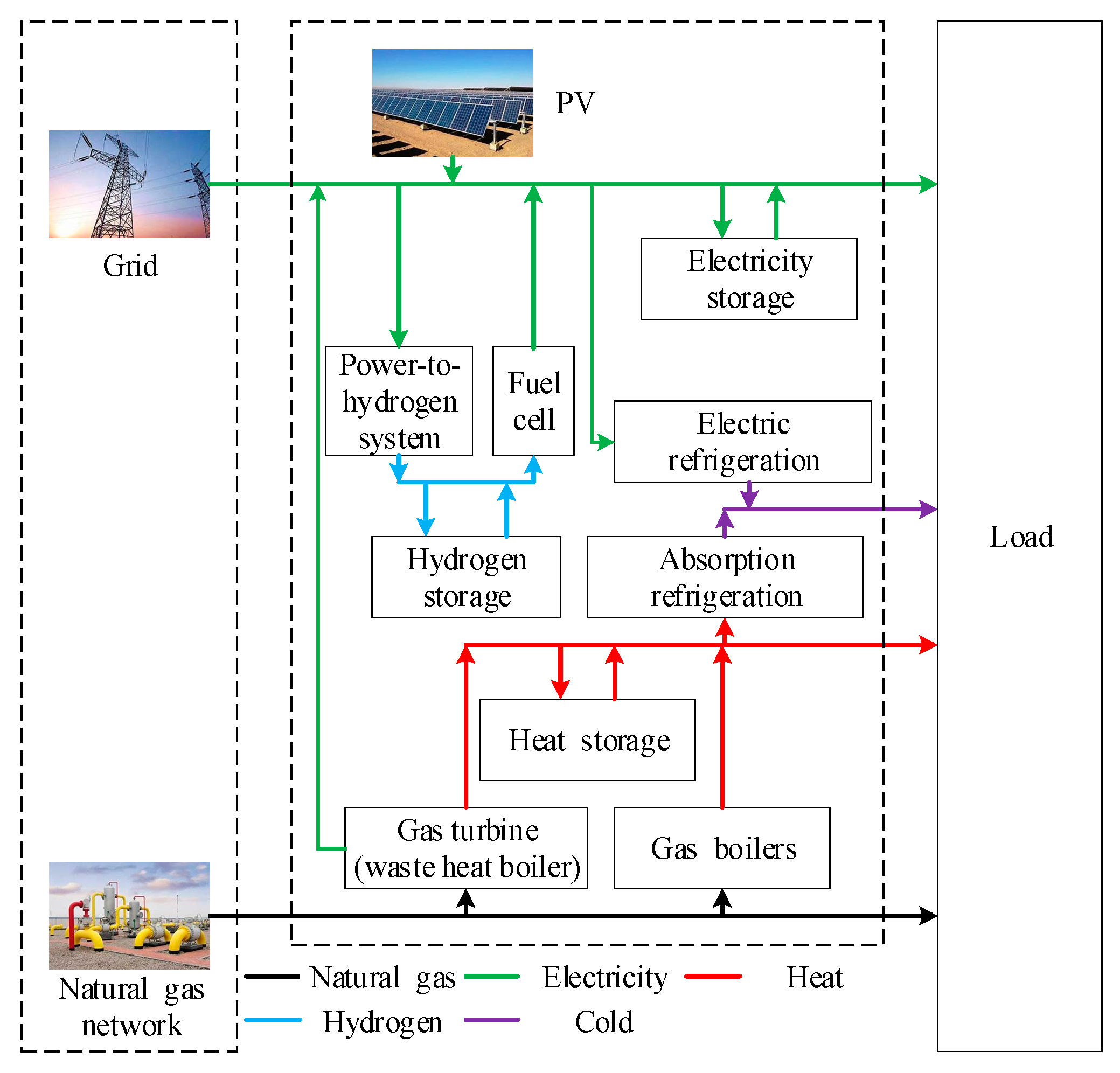
2.1. Analysis of IES

The IES integrates electricity, heat, cold, natural gas, and hydrogen, which can be used efficiently through energy management and optimal dispatching. This paper takes an industrial community IES as the research object, whose energy supply structure is shown in Figure 1.

The system includes four parts: energy supply, energy conversion equipment, energy storage equipment, and load:

• Energy supply includes a power grid, natural gas network, and PV, through which energy can be provided to the IES.
• Energy conversion equipment includes gas turbines and waste heat boilers, gas boilers, absorption refrigeration, electric refrigeration, power-to-hydrogen systems, and fuel cells, through which energy conversion is allowed so that one form of energy converts to another and meets the energy needs of IES.
• Energy storage equipment includes electricity storage, heat storage, and hydrogen storage. By using energy storage equipment, it is possible to transfer energy usage over time and increase the efficiency of energy consumption.
• Loads include electric, heat, cooling, and gas loads. They are the energy-using units of the IES.

2.2. Model of IES Equipment

2.2.1. Energy Supply

The mathematical model of the equipment developed in this paper and the corresponding parameters taken are referenced from [19,20].

1.

Pipe network for energy purchase

The customer purchases electricity from the grid via lines and transformers and purchases gas through the gas network feeder pipeline, which generally satisfies the line constraints [19],

$$P_{\mathrm{grid},\min ,x}^t⩽P_{\mathrm{grid},x}^t⩽P_{\mathrm{grid},\max ,x}^t$$

(1)

where $P_{grid,max,x,}^t$ and $P_{grid,min,x}^t$ are the upper and lower limits of the power transmitted for the electricity or gas supply at time t; t is the dispatch time; x is the energy type; e is the electrical energy; and g is the natural gas.

2.

PV

There are various model description methods for the output of PV, such as ideal circuit models and single-diode equivalent circuit models. Still, the models are complex to solve and unsuitable for engineering calculations. Therefore, a practical calculation model for photovoltaic equipment is modeled based on existing research [19].

$$I_{\mathrm{L}}=I_{\mathrm{sc}}\{1-A_1[\exp (\frac{U_{\mathrm{L}}-∆U}{A_2{U}_{\mathrm{oc}}})-1]\}$$

(2)

With Equation (2), the relationship between the output voltage and current of PV is approximately described, and some variables are calculated as follows:

$$\left\{\begin{array}{l}{A}_1=(1-\frac{I_{\mathrm{m}}}{I_{\mathrm{sc}}})\exp (-\frac{U_{\mathrm{m}}}{A_2{U}_{\mathrm{oc}}})\\ A_2=\frac{U_{\mathrm{m}}}{U_{\mathrm{oc}}-1}\cdot \frac{1}{\ln (1-\frac{I_{\mathrm{m}}}{I_{\mathrm{sc}}})}\\ ∆T=T-T_{\mathrm{ref}}\\ ∆I=\alpha (\frac{S}{S_{\mathrm{ref}}})∆T+(\frac{S}{S_{\mathrm{ref}}}-1)I_{\mathrm{sc}}\\ ∆U=-\beta ∆T-R_{\mathrm{s}}∆I\end{array}\right.$$

(3)

where I_sc is the short circuit current; U_oc is the open circuit voltage; I_m is the maximum power point current; U_m is the maximum power point voltage; S is the actual radiation intensity; T is the actual temperature; S_ref and T_ref are the reference values of radiation intensity and temperature; α and β are the current and voltage temperature coefficients under the reference radiation intensity, respectively, generally given in the product specification.

In practice, PV equipment is usually operated at the maximum power point to maximize the use of PV power. Therefore, it can be seen as a power source in optimal dispatching for IES.

2.2.2. Energy Conversion Equipment

1.

Gas turbines and waste heat boilers

The model of gas turbines and waste heat boilers is shown in the following equation [20]:

$$\begin{array}{l}{P}_{\mathrm{GT}}^t={\eta }_{\mathrm{GT},\mathrm{E}}{L}_{\mathrm{GAS}}{G}_{\mathrm{GT}}^t\\ H_{\mathrm{GT}}^t={\eta }_{\mathrm{GT},\mathrm{H}}(1-{\eta }_{\mathrm{GT},\mathrm{E}})L\mathrm{GAS}{G}_{\mathrm{GT}}^t\end{array}$$

(4)

where $P_{\mathrm{GT}}^t$ is the power produced by the gas turbine; η_{GT, E} is the power production efficiency; L_GAS is the low-level heat value of natural gas; $G_{GT}^t$ is the natural gas consumption rate; $H_{\mathrm{GT}}^t$ is the heat power generated from the gas turbine recovery; η_GT,H is the heat recovery efficiency.

2.

Gas boilers

A gas boiler produces steam by burning natural gas, and its model and operating constraints are shown in the equation below [19].

$$H_{\mathrm{GB}}^t={\eta }_{\mathrm{GB}}{L}_{\mathrm{GAS}}{G}_{\mathrm{GB}}^t$$

(5)

where $H_{\mathrm{GB}}^t$ is the heat production power of the gas boiler; η_GB is the heat production efficiency; $G_{\mathrm{GB}}^t$ is the natural gas consumption rate.

3.

Absorption refrigeration

Lithium bromide units can use high-temperature flue gas for cooling, with the model and operating constraints shown in the equation below [20].

$$C_{\mathrm{AC}}^t=c_{\mathrm{AC}}^{\mathrm{op}}{H}_{\mathrm{AC}}^t$$

(6)

where $C_{\mathrm{AC}}^t$ and $H_{\mathrm{AC}}^t$ are the absorption refrigerator’s cooling power and heat consumption power, respectively, and $c_{\mathrm{AC}}^{\mathrm{op}}$ is the energy efficiency ratio.

4.

Electric refrigeration

Electric refrigeration mainly refers to equipment such as central air conditioners, whose basic model and operating constraints are shown in the following equation [19]:

$$C_{\mathrm{EC}}^t=c_{\mathrm{EC}}^{\mathrm{op}}{P}_{\mathrm{EC}}^t$$

(7)

where $C_{EC}^t$ and $P_{EC}^t$ are the cooling power and power consumption of the electric refrigeration, respectively, and $c_{\mathrm{EC}}^{\mathrm{op}}$ is the energy efficiency ratio.

5.

Power-to-hydrogen system

The power-to-hydrogen system converts electrical energy into hydrogen through the electrolysis of water, with the simplified model and operational constraints shown in the following equation [20]:

$$H{H}_{\mathrm{EL}}^t={\eta }_{\mathrm{EL}}{P}_{\mathrm{EL}}^t$$

(8)

where ${HH}_{\mathrm{EL}}^t$ and $P_{\mathrm{EL}}^t$ are the hydrogen production power and power consumption of the power-to-hydrogen system, respectively, and η_EL is the hydrogen production efficiency.

6.

Fuel cells

The model and operating constraints of a fuel cell, which generates electrical energy through a chemical reaction, are shown in the following equation [20]:

$$P_{\mathrm{FC}}^t={\eta }_{\mathrm{FC}}H{H}_{\mathrm{FC}}^t$$

(9)

where $P_{\mathrm{FC}}^t$ and ${HH}_{\mathrm{FC}}^t$ are the fuel cell power production and hydrogen consumption power, respectively, and η_FC is the power production efficiency.

2.2.3. Energy Storage Equipment

Energy storage equipment can store energy through a medium and release it when needed. In this way, the spatial and temporal distribution of energy is changed. Traditionally, energy storage in power systems mainly refers to electrical energy storage. With the development of phase change energy storage and electrical hydrogen production technology, heat and hydrogen storage technologies have made great strides in recent years and have been gradually promoted for application. The operational dispatching model of energy storage equipment for multiple energy forms in a multi-energy complementary system is given here:

$$S_x^t=(1-{\sigma }_x)S_x^{t-1}+({\eta }_{x,\mathrm{c}}{P}_{x,\mathrm{c}}^t-\frac{P_{x,\mathrm{d}}^t}{{\eta }_{x,\mathrm{d}}})∆t$$

(10)

where $S_x^t$ and $S_x^{t-1}$ represent the energy storage’s remaining energy at the end of periods t and t − 1; σ_x is the self-loss factor of energy storage; η_x,c and η_x,d are the charging and discharging efficiencies; P_x,c and P_x,d are the charging and discharging power of the energy storage equipment, where x is e, h, and hh for electricity storage, heat storage, and hydrogen storage.

3. Model of Source–Load Uncertainty

3.1. Source–Load Prediction Error Uncertainty Model

For modeling PV and load uncertainties in IESs, their actual values can consist of two components [21]—the sum of the forecast value and the forecast error—expressed as follows.

$$\left\{\begin{array}{c}{P}_{\mathrm{PV}}^t=P_{\mathrm{PV},\mathrm{pre}}^t+∆P_{\mathrm{PV},\mathrm{pre}}^t\\ P_{\mathrm{load}}^t=P_{\mathrm{load},\mathrm{pre}}^t+∆P_{\mathrm{load},\mathrm{pre}}^t\end{array}\right.$$

(11)

where $P_{\mathrm{PV}}^t$ and $P_{\mathrm{load}}^t$ are the actual values of PV output and load; $P_{\mathrm{PV},\mathrm{pre}}^t$ and $P_{\mathrm{load},\mathrm{pre}}^t$ are the predicted values of PV output and load; Δ$P_{\mathrm{PV},\mathrm{pre}}^t$ and Δ$P_{\mathrm{load},\mathrm{pre}}^t$ are the prediction errors of PV output and load.

In general, the prediction error of PV output obeys a normal distribution with the mathematical expectation of 0 and standard deviation of ${\sigma }_{\mathrm{PV}}^t$, i.e., ${∆P}_{\mathrm{PV},\mathrm{pre}}^t$~N(0,${\sigma }_{\mathrm{PV}}^t$). Meanwhile, referring to related literature, the error of load prediction also obeys a normal distribution with the mathematical expectation of 0, i.e., ${∆P}_{\mathrm{load},\mathrm{pre}}^t$~N(0,${\sigma }_{\mathrm{load}}^t$) [22,23].

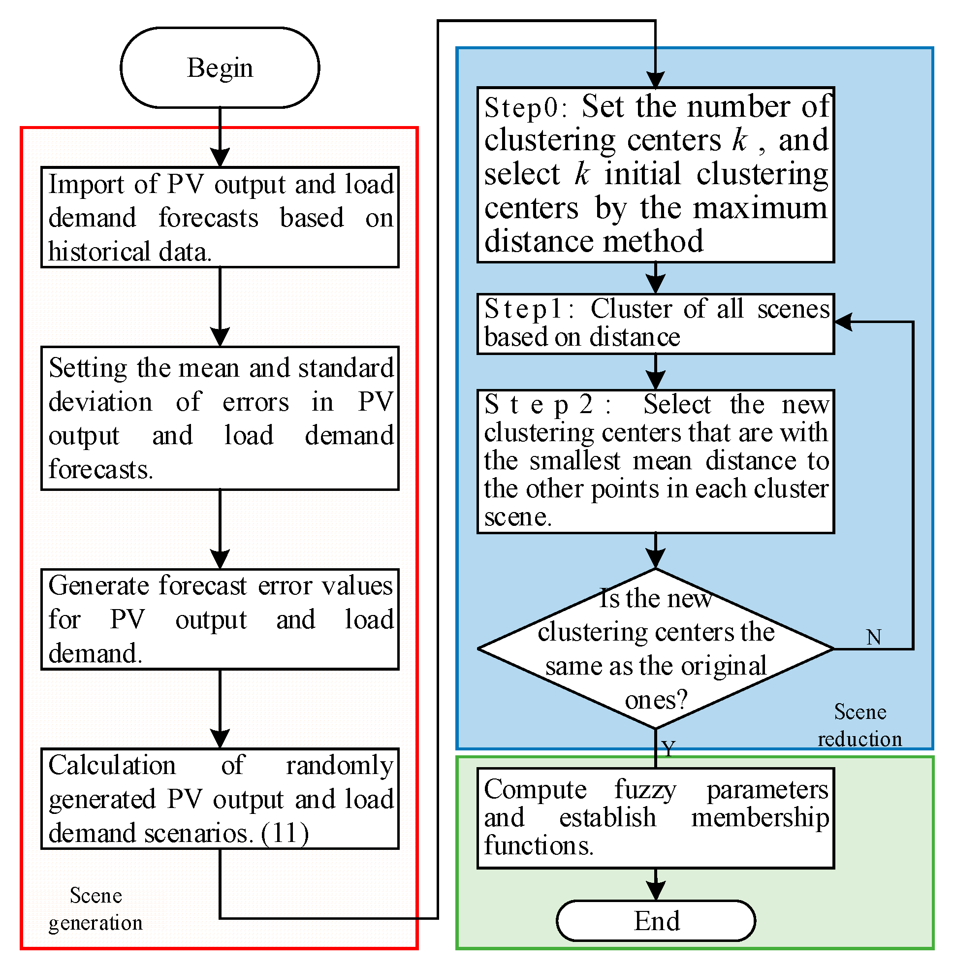
3.2. Source–Load Uncertainty Scenario Set Generation

Once the range of fluctuations for the source and load is determined, we can understand the uncertainty associated with the source and load. However, this method is still not precise enough. Therefore, building upon Section 3.1, the authors establish a typical scenario set for the source and load uncertainty. By constructing membership functions and utilizing fuzzy parameters, the uncertainty of the source and load is accurately modeled.

Because of its principle [19], the Monte Carlo simulation method can easily deal with many uncertainties in the power grid. Additionally, the computation time does not increase dramatically as the system size or the complexity of network connections increases. Therefore, in this paper, the Monte Carlo simulation method approach is used to generate many source–load uncertainty scenes and reduce them by K-means clustering of scenes.

In this paper, an improved K-means clustering algorithm based on the maximum distance method is used. The processing of the K-means clustering algorithm is shown in Alogorithm 1 [24].

Alogorithm 1. The processing of the K-means clustering algorithm.

Step 1. Initialization. Set the number of clustering centers k, and select k initial clustering centers by the maximum distance method. The specific steps are as follows. Step 1.1. Select the 2 scenes with the greatest distance in the scene set as the initial clustering centers. Step 1.2. Select other k − 2 clustering centers. Among the remaining N − 2 scenes, the scene with the largest distance product to the first two initial scenes is selected as the third cluster center. Through this method, k initial cluster centers are obtained. Step 2. Calculate the Euclidean distance of each object to each clustering center, compare the distance of each object to each clustering center in turn, and assign the object to the class cluster of the nearest clustering center to obtain k class clusters {S1, S2, S3, …, Sk}. Step 3. The object with the smallest mean value of the Euclidean distance from other objects in each class cluster is selected as the new clustering cente. Step 4. Judgment. Step 4.1. If the new clustering center is different from the previous clustering center, repeat Step 2–Step 3. Step 4.2. If the new clustering center is the same as the previous one, end.

In the K-means clustering algorithm, K is selected by the elbow method [25,26]. The principle of the elbow method is as follows. The sum of the squares of the Euclidean distances between the samples of each cluster and the average values of all samples in that cluster is calculated, denoted as [h₁, h₂, …, h_k]. Their sum is denoted as H and represents the clustering effect under the current K. The smaller the value of H, the better the clustering effect. We will calculate H at different K starting from K = 1 and plot them into the figure. When the absolute value of the slope of the curve suddenly decreases, the corresponding K is the optimal value.

In summary, the process for generating a typical set of scenarios for uncertainty and calculating the fuzzy parameters is shown in Figure 2.

4. IES Optimization Dispatching Model

4.1. Objective Function

For the community, the objective function for its optimal dispatch is the minimized daily operating cost, which consists of three components—energy cost, equipment operation and maintenance cost, and curtailment penalty cost—denoted as:

$$C=C_{\mathrm{op}}+C_{\mathrm{om}}+C_{\mathrm{adpv}}$$

(12)

where C_op is the system’s energy cost; C_om is the system’s equipment operation and maintenance cost; C_adpv is the system’s curtailment penalty cost.

The energy cost C_op is the cost of electricity and natural gas purchased by the IES from the upper grid and the natural gas network, expressed as:

$$C_{\mathrm{op}}={\displaystyle \sum _{t=1}^T(y_{\mathrm{e}}^t{P}_{\mathrm{grid},\mathrm{e}}^t+y_{\mathrm{g}}^t{P}_{\mathrm{grid},\mathrm{g}}^t)∆t}$$

(13)

where $y_{\mathrm{e}}^t$ is the price of electricity purchased from the grid in time t; $y_{\mathrm{g}}^t$ is the price of natural gas purchased from the natural gas grid in time t; $P_{\mathrm{grid},\mathrm{e}}^t$ is the power purchased from the superior grid in time t. Additionally, $P_{\mathrm{grid},\mathrm{g}}^t$ is the power of natural gas purchased from the natural gas grid in time t; T is the number of dispatching periods, 1 h, in Equation (14).

The equipment operation and maintenance cost is the cost incurred during the use of equipment in an IES and is expressed as:

$$C_{\mathrm{om}}={\displaystyle \sum _{t=1}^T{\displaystyle \sum _{i=1}^G{c}_{\mathrm{om},i}{P}_i^t∆t}}$$

(14)

where c_om,i is the operation and maintenance cost per unit power output of equipment i; $P_i^t$ is the output power of equipment i at time t; G is the set of equipment; and i denotes the equipment type.

The penalty cost is a penalty for the community’s failure to fully use the new energy source. This paper introduces a segmented penalty factor for the widespread solar power curtailment phenomenon [27,28,29]. As the amount of PV power curtailment increases, the penalty factor also increases, and a time-of-use tariff coefficient is introduced to adopt a segmented penalty cost related to both the tariff and the power curtailed, expressed as follows:

$$C_{\mathrm{adpv}}={\displaystyle \sum _{t=1}^T{c}_{\mathrm{adpv}}^t{y}_{\mathrm{e}}^t{W}_{\mathrm{PV}}^t∆t}$$

(15)

where $W_{\mathrm{PV}}^t$ is the discarded power of the system at time t, and $c_{\mathrm{adpv}}^t$ is the discard penalty factor of the system, which is related to the discard rate of the system and is expressed as

$$c_{\mathrm{adpv}}^t=\left\{\begin{array}{cc}0.75& 0\le {\alpha }_{\mathrm{PV}}^t\le 3\%\\ 1.5& {\alpha }_{\mathrm{PV}}^t>3\%\end{array}\right.$$

(16)

where ${\alpha }_{\mathrm{PV}}^t$ is the curtailment rate of the system at time t.

As can be seen in Equation (16), due to the introduction of segmented curtailment costs, the community tends to make fuller use of photovoltaic power generation when electricity prices are higher, which not only helps reduce new energy waste and promote local absorption but also helps reduce the daily peak-to-valley difference in the community’s electricity consumption and reduce the impact on the grid.

4.2. Constraints

4.2.1. Energy Balance Constraints

The system needs to meet all of the loads to ensure normal operation. Therefore, the energy generated by the equipment and input to the energy flow from outside needs to be equal to the energy required to use the equipment and meet the load demand during operation, which is the energy power balance constraint.

1.

Electrical Balance

$$P_{\mathrm{grid},\mathrm{e}}^t+P_{\mathrm{use},\mathrm{PV}}^t+P_{\mathrm{GT}}^t+P_{\mathrm{FC}}^t+P_{\mathrm{e},\mathrm{d}}^t=P_{\mathrm{EC}}^t+P_{\mathrm{EL}}^t+P_{\mathrm{e},\mathrm{c}}^t+P_{\mathrm{load}}^t$$

(17)

where $P_{\mathrm{grid},\mathrm{e}}^t$ is the power transmitted from the outside; $P_{\mathrm{use},\mathrm{PV}}^t$ is the PV power utilized by the IES at time t; $P_{\mathrm{GT}}^t$ is the power produced by the gas turbine; $P_{\mathrm{FC}}^t$ is the production power of the fuel cell; $P_{\mathrm{e},\mathrm{d}}^t$ is the discharging power of the electricity storage; $P_{\mathrm{EC}}^t$ is the power consumption of the electric refrigeration; $P_{\mathrm{EL}}^t$ is the power consumption of the power-to-hydrogen system; $P_{\mathrm{e},\mathrm{c}}^t$ is the charging power of the electricity storage; $P_{\mathrm{load}}^t$ is the electrical load of the IES at time t.

The electrical power input to the IES includes purchasing power from the grid, power generation of PV, power generation of gas turbines, power generation of fuel cells, and discharge power of electricity storage, as shown on the left side of Equation (17). The ways of outputting electric power from the IES include electricity for electric refrigeration, power-to-hydrogen system, the charge of electricity storage, and meeting the electric load, as shown on the right side of Equation (17).

2.

Heat Balance

$$H_{\mathrm{GT}}^t+H_{\mathrm{GB}}^t+P_{\mathrm{h},\mathrm{d}}^t=H_{\mathrm{AC}}^t+P_{\mathrm{h},\mathrm{c}}^t+H_{\mathrm{load}}^t$$

(18)

where $H_{\mathrm{GT}}^t$ is the heat power generated from the gas turbine recovery; $H_{\mathrm{GB}}^t$ is the heat production power of the gas boiler; $P_{\mathrm{h},\mathrm{d}}^t$ is the discharging power of the heat storage; $H_{\mathrm{AC}}^t$ is the absorption refrigerator’s heat consumption power; $P_{\mathrm{h},\mathrm{c}}^t$ is the charging power of the heat storage; $H_{\mathrm{load}}^t$ is the heat load of the IES at time t.

The input of heat to the IES includes the generation of gas turbines, generation of gas billers, and discharge of heat storage, as shown on the left side of Equation (18). The ways of outputting heat from the IES include using absorption refrigeration, the charge of heat storage, and meeting the heat load, as shown on the right side of Equation (18).

3.

Cold Balance

$$C_{\mathrm{AC}}^t+C_{\mathrm{EC}}^t=C_{\mathrm{load}}^t$$

(19)

where $C_{\mathrm{AC}}^t$ is the absorption refrigerator’s cooling power; $C_{\mathrm{EC}}^t$ is the cooling power of electric refrigeration; $C_{\mathrm{load}}^t$ is the cooling load of the IES at time t.

The input of clod to the IES includes the generation of electric refrigeration and absorption refrigeration, as shown on the left side of Equation (19). The way of outputting clod from the IES is meeting the cooling load, as shown on the right side of Equation (19).

4.

Natural Gas Balance

$$P_{\mathrm{grid},\mathrm{g}}^t=L_{\mathrm{GAS}}(G_{\mathrm{GT}}^t+G_{\mathrm{GB}}^t+G_{\mathrm{load}}^t)$$

(20)

where $P_{\mathrm{grid},\mathrm{g}}^t$ is the natural gas transmitted from the outside; $G_{\mathrm{GT}}^t$ is the natural gas consumption rate; $G_{\mathrm{GB}}^t$ is the natural gas consumption rate; L_GAS is the low-level heat value of natural gas; $G_{\mathrm{load}}^t$ is the natural gas load of the IES at time t.

The input of gas to the IES is the purchase from the outside, as shown on the left side of Equation (20). The ways of outputting gas from the IES are using gas turbines and gas billers, as shown on the right side of Equation (20).

5.

Hydrogen Balance

$$H{H}_{\mathrm{EL}}^t+P_{\mathrm{hh},\mathrm{d}}^t=H{H}_{\mathrm{FC}}^t+P_{\mathrm{hh},\mathrm{c}}^t$$

(21)

where ${HH}_{\mathrm{EL}}^t$ is the hydrogen production power of the power-to-hydrogen system; $P_{\mathrm{h}\mathrm{h},\mathrm{d}}^t$ is the discharging power of the hydrogen storage; ${HH}_{\mathrm{FC}}^t$ is the fuel cell’s hydrogen consumption power; $P_{\mathrm{h}\mathrm{h},\mathrm{c}}^t$ is the charging power of the hydrogen storage.

The hydrogen input to the IES includes the generation of the power-to-hydrogen system and discharge of hydrogen storage, as shown on the left side of Equation (21). The ways of outputting hydrogen from the IES include using fuel cells and charge of hydrogen storage, as shown on the right side of Equation (21).

4.2.2. Equipment Working Conditions Constraints

1.

Equipment Output Constraints

In addition to the line constraints for pipe network for energy purchase, as described in Equation (1), the output power of each piece of equipment should also meet the upper and lower limits of the equipment output constraints.

$$\left\{\begin{array}{l}{P}_{\mathrm{GT},\min }^{}\le P_{\mathrm{GT}}^t\le P_{\mathrm{GT},\max }^{}\hfill \\ H_{\mathrm{GB},\min }^{}\le H_{\mathrm{GT}}^t\le H_{\mathrm{GB},\max }^{}\hfill \\ C_{\mathrm{AC},\min }^{}\le C_{\mathrm{AC}}^t\le C_{\mathrm{AC},\max }^{}\hfill \\ C_{\mathrm{EC},\min }^{}\le C_{\mathrm{EC}}^t\le C_{\mathrm{EC},\max }^{}\hfill \\ H{H}_{\mathrm{EL},\min }^{}\le H{H}_{\mathrm{EL}}^t\le H{H}_{\mathrm{EL},\max }^{}\hfill \\ P_{\mathrm{FC},\min }^{}\le P_{\mathrm{FC}}^t\le P_{\mathrm{FC},\max }^{}\hfill \\ 0\le P_{x,\mathrm{c}}^t\le P_{x,\mathrm{c},\max }^{}\hfill \\ 0\le P_{x,\mathrm{d}}^t\le P_{x,\mathrm{d},\max }^{}\hfill \end{array}\right.$$

(22)

2.

Equipment Power Ramp Rate Constraints

For gas turbines with waste heat boilers, gas boilers, and power-to-hydrogen systems, the power ramp rate should be constrained when operating, i.e.,

$$\left\{\begin{array}{l}{P}_{\mathrm{GT}}^{t+1}-P_{\mathrm{GT}}^t\le ∆P_{\mathrm{GT}}^{}\hfill \\ H_{\mathrm{GB}}^{t+1}-H_{\mathrm{GB}}^t\le ∆H_{\mathrm{GB}}^{}\hfill \\ H{H}_{\mathrm{EL}}^{t+1}-H{H}_{\mathrm{EL}}^t\le ∆H{H}_{\mathrm{EL}}^{}\hfill \end{array}\right.$$

(23)

where ΔP_GT is the maximum power ramp rate of the gas turbine and waste heat boilers; ΔH_GB is the maximum power ramp rate of the gas boilers; ΔHH_EL is the maximum power ramp rate of the power-to-hydrogen systems.

3.

Energy Storage Operating Mode Constraints

For energy storages, it should be ensured that they cannot be in charging and discharging states at the same time, and, therefore, the operating mode of the energy storages should be further constrained based on Equation (24), i.e.,

$$\left\{\begin{array}{c}0\le P_{x,\mathrm{c}}^t\le v_{x,\mathrm{c}}{P}_{x,\mathrm{c},\max }^{}\\ 0\le P_{x,\mathrm{d}}^t\le v_{x,\mathrm{d}}{P}_{x,\mathrm{d},\max }^{}\\ v_{x,\mathrm{c}}+v_{x,\mathrm{d}}\le 1\end{array}\right.$$

(24)

where v_x,c and v_x,d are the energy storage’s charging and discharging working mode markers. When v_x,c = 1, the energy storage is in the charging state; when v_x,d = 1, it means the energy storage is discharging. Three working modes of energy storage can be specified through the above constraints: charging only, discharging, and no charging without discharging.

4.2.3. Curtailment Rate Constraints

To maximize PV absorption and minimize curtailment, the curtailment rate under this model is constrained:

$$R_{\mathrm{PV}}^t\le \theta$$

(25)

where $R_{\mathrm{PV}}^t$ is the curtailment rate of the system at time t, and θ is the upper limit of the curtailment rate of the system.

4.2.4. Reliability Constraints

A method of stochastic dispatching is proposed, known as chance constraint planning, which is used to handle source–load uncertainty variables. It involves creating fuzzy chance constraints that allow for optimization results that may not fully meet the constraints and may even violate them to a certain probability. However, the probability of the constraints being met must be equal to or greater than the set confidence level.

The uncertainty factors considered In this paper are PV output at various times and fluctuations in electricity, natural gas, heat, and cooling load. The power balance constraint is bounded at a certain confidence level to cope with the impact of the uncertainty factors on the system dispatch results and to balance the system operation economy and reliability to a certain extent. The system power reliability constraints for electricity, natural gas, heat, and cooling are the following:

$$P[P_{\mathrm{grid},\mathrm{e}}^t+\left(P_{\mathrm{PV},\mathrm{pre}}^t+∆P_{\mathrm{PV},\mathrm{pre}}^t\right)+P_{\mathrm{GT}}^t+P_{\mathrm{FC}}^t+P_{\mathrm{e},\mathrm{d}}^t\ge \left(P_{\mathrm{Pload},\mathrm{pre}}^t+∆P_{\mathrm{Pload},\mathrm{pre}}^t\right)+P_{\mathrm{EC}}^t+P_{\mathrm{EL}}^t+P_{\mathrm{e},\mathrm{c}}^t]\ge \beta$$

(26)

$$P[H_{\mathrm{GT}}^t+H_{\mathrm{GB}}^t+P_{\mathrm{h},\mathrm{d}}^t\ge H_{\mathrm{AC}}^t+P_{\mathrm{h},\mathrm{c}}^t+\left(P_{\mathrm{Hload},\mathrm{pre}}^t+∆P_{\mathrm{Hload},\mathrm{pre}}^t\right)]\ge \beta$$

(27)

$$P[C_{\mathrm{AC}}^t+C_{\mathrm{EC}}^t\ge P_{\mathrm{Cload},\mathrm{pre}}^t+∆P_{\mathrm{Cload},\mathrm{pre}}^t]\ge \beta$$

(28)

$$P[P_{\mathrm{grid},\mathrm{g}}^t\ge L_{\mathrm{GAS}}(G_{\mathrm{GT}}^t+G_{\mathrm{GB}}^t)+\left(P_{\mathrm{Gload},\mathrm{pre}}^t+∆P_{\mathrm{Gload},\mathrm{pre}}^t\right)]\ge \beta$$

(29)

where $P_{\mathrm{PV},\mathrm{pre}}^t$, $P_{\mathrm{Pload},\mathrm{pre}}^t$, $P_{\mathrm{Hload},\mathrm{pre}}^t$, $P_{\mathrm{Cload},\mathrm{pre}}^t$, and $P_{\mathrm{Gload},\mathrm{pre}}^t$ are forecasts of PV output, electrical load, heat load, cooling load, and natural gas load; Δ$P_{\mathrm{PV},\mathrm{pre}}^t$, Δ$P_{\mathrm{Pload},\mathrm{pre}}^t$, Δ$P_{\mathrm{Hload},\mathrm{pre}}^t$, Δ$P_{\mathrm{Cload},\mathrm{pre}}^t$, and Δ$P_{\mathrm{Gload},\mathrm{pre}}^t$ are forecast errors of PV output, electrical load, heat load, cooling load, and natural gas load; and β is the confidence level.

In this paper, the fuzzy variables are PV output and electric, heat, cold, and natural gas loads. Then, the uncertain constraints are converted into deterministic constraints using the method cited in [30,31]. If β > 0.5, the uncertain constraints such as Equation (30) can be converted, as shown in Equation (31). If β < 0.5, the uncertain constraints can be converted, as shown in Equation (32).

$$P[{\tilde{P}}_x-{\tilde{P}}_y\le \mathit{k}]\ge \beta$$

(30)

$$-\mathit{k}+(2-2\beta ){\tilde{P}}_x+(2\beta -1)k_{x,u}{\tilde{P}}_x-(2-2\beta ){\tilde{P}}_y-(2\beta -1)k_{y,u}{\tilde{P}}_y\le 0$$

(31)

$$-\mathit{k}+(1-2\beta )k_{x,l}{\tilde{P}}_x+2\beta {\tilde{P}}_x-(1-2\beta )k_{y,l}{\tilde{P}}_y-2\beta {\tilde{P}}_y\le 0$$

(32)

where ${\tilde{P}}_x$ and ${\tilde{P}}_y$ are the fuzzy variables; k is the set of certain variables; k_x,u, k_y,u, k_x,l, and k_y,l are the parameters of the fuzzy membership function.

Taking Equation (26) as an example, if β > 0.5, the equation can be converted into Equation (33). If β < 0.5, the equation can be converted into Equation (34).

$$-(P_{\mathrm{grid},\mathrm{e}}^t+P_{\mathrm{GT}}^t+P_{\mathrm{FC}}^t+P_{\mathrm{e},\mathrm{d}}^t-P_{\mathrm{EC}}^t-P_{\mathrm{EL}}^t-P_{\mathrm{e},\mathrm{c}}^t)+(2-2\beta ){\tilde{P}}_{\mathrm{PV}}^t+(2\beta -1)k_{\mathrm{PV},\mathrm{u}}{\tilde{P}}_{\mathrm{PV}}^t-(2-2\beta ){\tilde{P}}_{\mathrm{Pload}}^t-(2\beta -1)k_{\mathrm{Pload},\mathrm{u}}{\tilde{P}}_{\mathrm{Pload}}^t\le 0$$

(33)

$$-(P_{\mathrm{grid},\mathrm{e}}^t+P_{\mathrm{GT}}^t+P_{\mathrm{FC}}^t+P_{\mathrm{e},\mathrm{d}}^t-P_{\mathrm{EC}}^t-P_{\mathrm{EL}}^t-P_{\mathrm{e},\mathrm{c}}^t)+(1-2\beta )k_{\mathrm{PV},\mathrm{l}}{\tilde{P}}_{\mathrm{PV}}^t+2\beta {\tilde{P}}_{\mathrm{PV}}^t-(1-2\beta )k_{\mathrm{Pload},\mathrm{l}}{\tilde{P}}_{\mathrm{Pload}}^t-2\beta {\tilde{P}}_{\mathrm{Pload}}^t\le 0$$

(34)

4.3. Solution Process

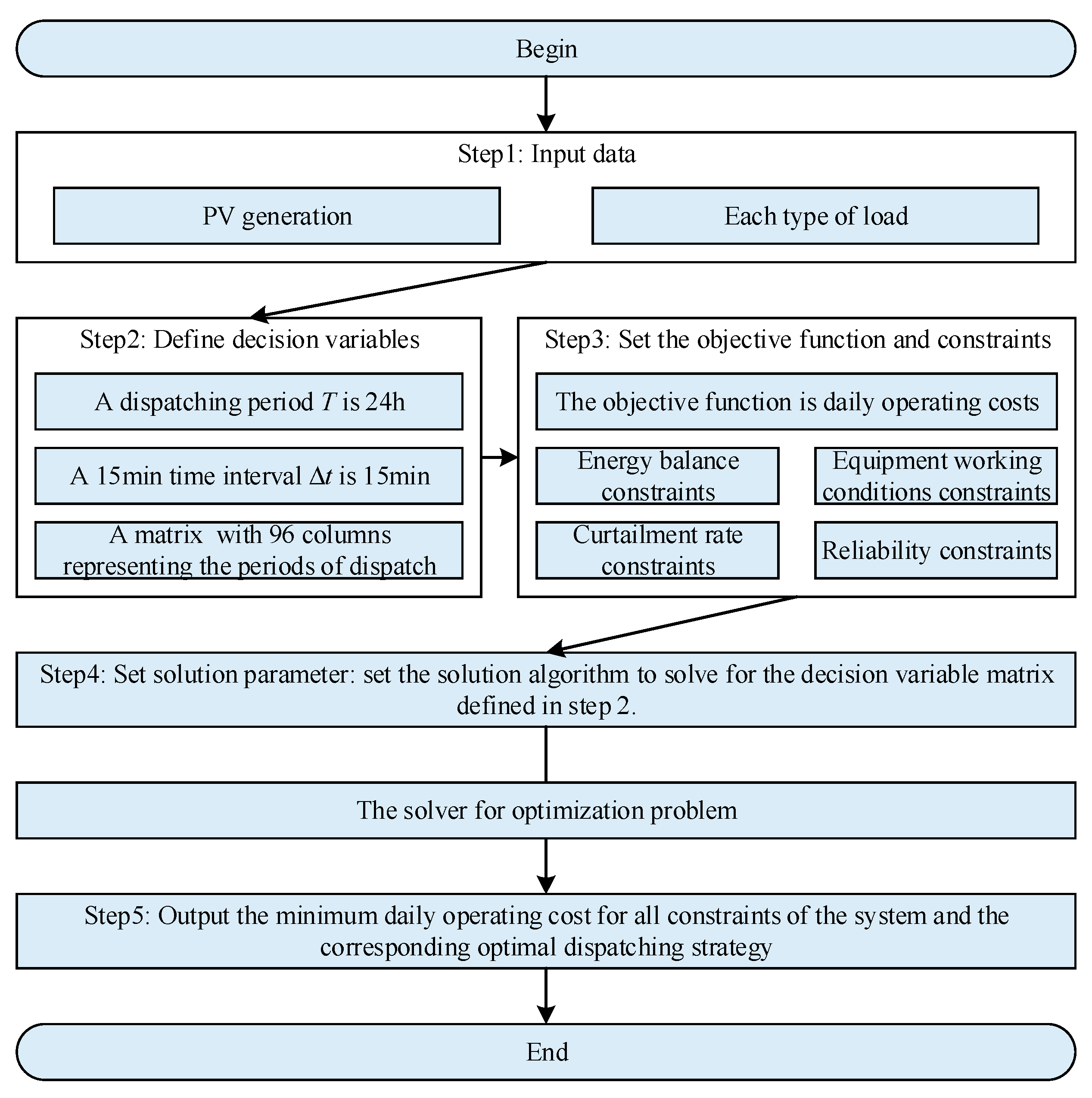
The IES is coupled with many types of equipment and has many optimization variables, which is essentially an MILP problem. The solution process of which is shown in Figure 3.

The details are as follows:

(1)

Input data. Based on the PV generation resource endowment of the community’s historical daily load data, input its PV generation and its corresponding data set for each type of load scenario, and input relevant data information for each equipment model.

(2)

Define the optimal dispatching decision variables. Let a 24 h day be a dispatching period. Define a matrix of decision variables x with columns 1 to 96 representing the 96 periods of the day, respectively.

(3)

Set the optimal dispatching objective function and constraints. The objective function is optimal daily operating costs. The constraints include each equipment model and the system power balance constraints.

(4)

Solution parameter setting. In this paper, the mathematical optimization toolkit YALMIP is used to model and then call the CPLEX solver to solve the problem to realize the optimization dispatching of multiple devices in the system.

(5)

Output. The optimization algorithm solves the minimum daily operating cost for all constraints of the system and the corresponding optimal dispatching strategy.

5. Case Analysis

5.1. The Parameters of IES and Case Settings

The equipment parameters for an actual IES community are shown in Appendix A.

This IES has the networks of electricity, heat, cold, natural gas, and hydrogen, and this example has been designed with the following arithmetic:

Case 1: Disregard the cost of curtailment penalties;

Case 2: Consider a non-segmented curtailment penalty cost; the expression of the curtailment penalty factor is

$$c_{\mathrm{adpv}}^{\prime }=1.275$$

(35)

Case 3: Consider using segmented solar power curtailment penalty costs as in Equation (16).

In these cases, to demonstrate the effect of the proposed segmented curtailment penalty cost, the community purchases electricity using a time-of-use electricity price, and the community purchases electricity from external sources at the prices shown in

Table 2. Time-of-use electricity price.

Time	Price (CNY/kWh)
00:00–06:59 22:00–23:59	0.48
07:00–10:59 14:00–17:59	0.88
11:00–13:59 18:00–21:59	1.10

[19,20].

The price of natural gas is 3.80 CNY/m³, which can be converted to 0.392 CNY/kWh based on the calorific value of natural gas (9.7 kWh/m³).

This optimization problem was solved on a computer with an Intel Core i7-8700 3.20 GHz processor and 16 GB of RAM in MATLAB R2020b, using the CPLEX 12.10.0 optimization solver.

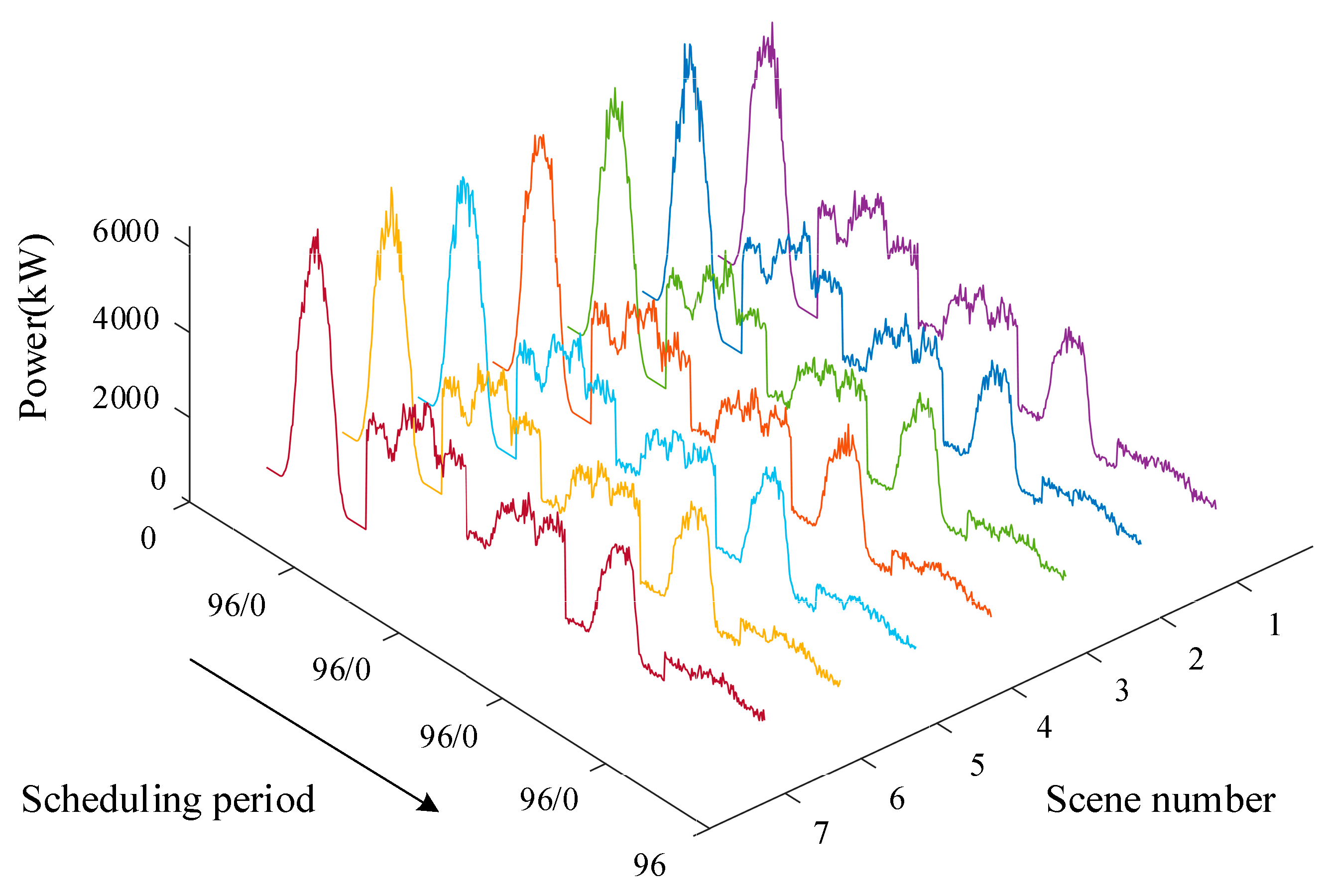
5.2. Scenario Set Generation

Based on historical data [19], the fuzzy parameters of the PV output and the load are shown in

Table A2. The fuzzy parameters for each scenario.

Scenario Number	Probability of Occurrence	kPV,l	kPV,u	kPload,l	kPload,u	kHload,l	kHload,u	kCload,l	kCload,u	kGload,l	kGload,u
1	24.86%	0.9196	1.0804	0.9504	1.0496	0.9702	1.0298	0.9698	1.0302	0.9502	1.0498
2	5.42%	0.9207	1.0793	0.9498	1.0502	0.9700	1.0300	0.9706	1.0294	0.9495	1.0505
3	11.16%	0.9200	1.0200	0.9501	1.0599	0.9702	1.0298	0.9701	1.0299	0.9497	1.0503
4	3.26%	0.9197	1.0803	0.9500	1.0500	0.9698	1.0302	0.9703	1.0297	0.9496	1.0503
5	18.81%	0.9196	1.0803	0.9505	1.0495	0.9697	1.0302	0.9700	1.0300	0.9503	1.0496
6	22.07%	0.9205	1.0795	0.9503	1.0497	0.9703	1.0297	0.9699	1.0301	0.9501	1.0499
7	14.42%	0.9197	1.0802	0.9498	1.0501	0.9699	1.0201	0.9702	1.0298	0.9498	1.0502
all	/	0.92	1.08	0.95	1.05	0.97	1.03	0.97	1.03	0.95	1.05

. Then, 5000 random scenarios are generated and clustered into serval typical scenarios, with the fuzzy parameters of each typical scenario calculated. The value of K is chosen as 7 using the elbow method. The clustering results are shown in Figure 4.

The dispatching periods are PV output, electrical load, natural gas load, cooling load, and heat load along the direction of the arrows. The seven typical scenarios are 24.86%, 5.42%, 11.16%, 3.26%, 18.81%, 22.07%, and 14.42%, respectively, covering all possible scenarios well.

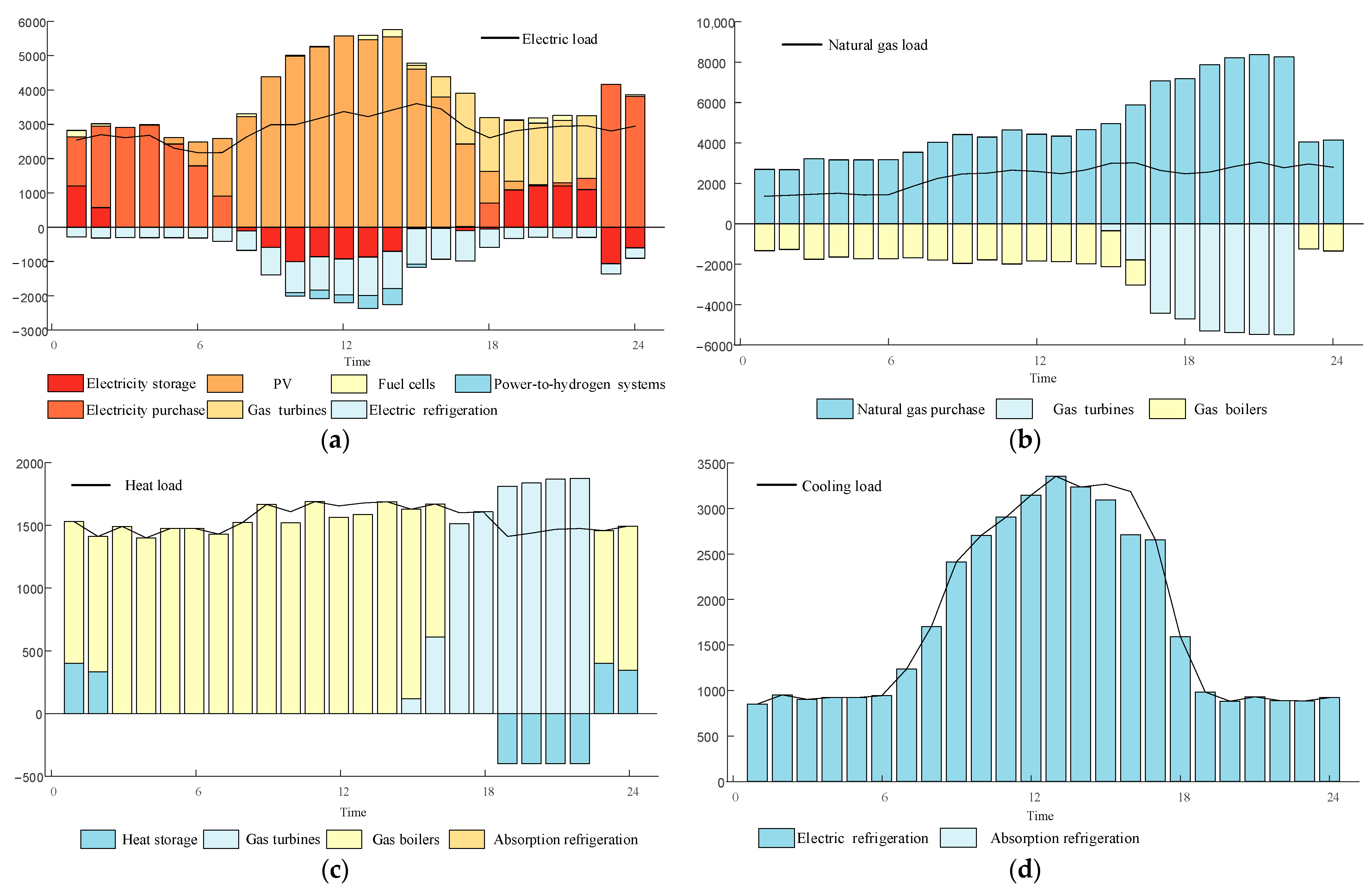
5.3. Analysis of Results

5.3.1. Economic Analysis of Different Cases

The optimal dispatching results for Cases 1 to 3 are shown in

Table 3. The optimal dispatching result.

Case	Cop	Com	Cadpv	C
1	52,791.87	8679.83	447.22	61,918.92
2	52,738.42	8783.74	173.35	61,695.51
3	52,729.85	8822.61	125.51	61,677.97

, where for Case 1, the curtailment penalty cost is taken as the average value of the two different calculation methods, at which point β = 0.95.

To determine the dispatching outcomes, the results of all scenarios in Figure 4 are weighted and shown in Table 2 for each case. To better quantify the operation status of various types of equipment with the changes in load size and electricity price, we will use Scenario 1 as an example for analysis, as it has the highest probability of occurring. The satisfaction of electric, natural gas, heat, and cooling load and the dispatching of equipment under Case 3 are shown in Figure 5. Additionally, the optimized operating results of 7 scenarios for Case 3 are shown in Appendix A.

Between 0:00 and 6:00, the electric load is mainly met by electricity purchased from the grid due to the low level of PV power. Between 6:00 and 19:00, PV is the primary source of electricity supply. Due to the surplus of electricity during most of the day caused by PV output, to accommodate more power locally, the electricity storage and the combined hydrogen network, consisting of a power-to-hydrogen system, hydrogen storage, and fuel cell tends to absorb electricity at the peak of the PV generation and release electricity at the trough of the PV generation to reduce the purchase of electricity.

The heat load is mainly supplied through gas boilers and heat storage. Between 16:00 and 22:00, the gas turbines are activated to supplement the power supply due to a lack of electrical energy supply, so the output of the gas boilers is reduced to maintain the heat balance during this period.

For the cooling load, the electric refrigeration is supplied exclusively by the electric refrigeration as their conversion energy efficiency is greater than that of the absorption refrigeration.

5.3.2. Economic Analysis of Different Confidence Levels

For Scenario 1 of Case 3, which reduces the system’s confidence level from 1 to 0.8, the performance of the system economy is shown in

Table 4. The daily operating cost of different confidence level.

β	C
1	62,478.82
0.95	61,325.70
0.9	53,838.67
0.85	47,489.64
0.8	42,025.44

.

The above table shows that the system’s economy gradually increases as the confidence level decreases. The daily operating cost decreases as the confidence level changes. However, as the change, the IES system is satisfying less and less of the load, leading to decreasing customer satisfaction with energy use. Therefore, it is necessary to select an appropriate confidence level.

Then, all of the source–load uncertainty scenes generated by the Monte Carlo sampling method are used to test the optimization dispatching model’s robustness in different confidence levels. The result is shown in

Table 5. The number of scenarios that can be solved at different confidence levels.

β	Num of Solvable Scenarios
1	4727
0.95	5000
0.9	5000
0.85	5000
0.8	5000

, and all scenes are solvable when the confidence level is smaller than 0.95. In practical applications, ensuring that the energy supply can meet the energy demand for as many time periods as possible is important. This means the probability of the balance constraints being met should be maximized. Additionally, as shown in Figure 5, there is no significant energy supply shortage when the confidence level is 0.95. Therefore, if the confidence level is 0.95, the system’s risks are controllable. We can also set a certain amount of backup energy capacity based on the optimization plan to cope with uncertainty. The robustness of the optimization dispatching model can guarantee practical application.

Moreover, in the manuscript, the authors adopt the source–load uncertainty scenario set generation first and the chance constraints to cope with the impact of source–load uncertainty. The model proposed in this paper combines scenario method modeling and chance-constrained planning modeling. When the confidence level is 1, the optimization dispatching model is the same as the model adopted by the scenario method. However, when testing it, it is not solvable for all of the scenes. Therefore, the scenario method still has a risk in the system’s operation, and we should adopt the chance constraints to cope with the impact of source–load uncertainty.

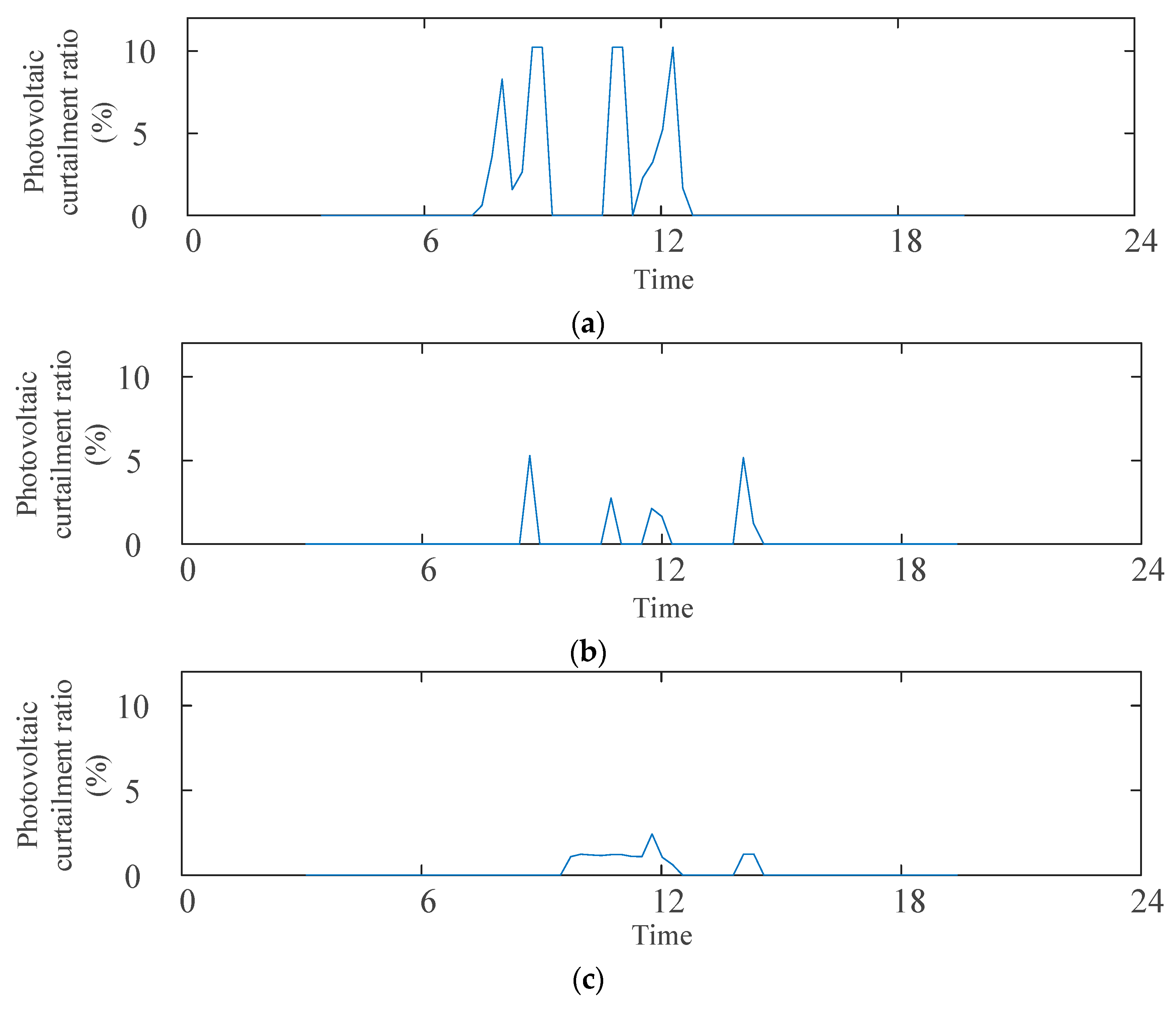
5.3.3. Analysis of The Phenomenon of Solar Power Curtailment

The peak curtailment rates in the three cases are 10%, 5.22%, and 2.40%, as shown in Figure 6.

For Case 1, which does not consider the curtailment penalty cost, the amount of PV curtailment is higher, reaching the upper limit of 10% of the curtailment rate specified by the system. Overall, due to the higher amount of PV curtailment, the system needs to spend more to purchase energy to meet the system’s energy demand, resulting in a higher total operating cost. For Case 2, which uses no segmentation of the curtailment penalty cost, the system only curtails PV between 11:00–12:00 and 14:00–15:00. In the rest of the time, the PV is effectively used. Therefore, the penalty cost drops significantly compared to Case 1 by 61.24%. In Case 3, the system tends to control the amount of curtailment. Still, since the curtailment amount is insignificant in all periods after dispatch, the curtailment penalty factor is 0.75, and the penalty cost is lower, further improving the system’s economy.

For Case 1, the system minimizes energy and equipment operation and maintenance costs as it does not consider the curtailment penalty cost. Therefore, the hydrogen network and energy storage are only dispatched to accommodate excess PV generation when the curtailment rate exceeds the limit.

For Case 2, compared to Case 3, due to its non-segmented curtailment penalty cost, the dispatching of the energy storage and hydrogen network is not limited to the period of maximum pressure for PV absorption but rather ensures the lowest total curtailment through dispatching.

Looking at the dispatching results of the three cases, it can be seen as follows:

1.

When the system only considers the cost of energy use and equipment operation and maintenance costs, the system pays a higher penalty cost for curtailment, and the cost of energy use increases because the system cannot fully utilize the PV and needs to purchase energy from outside the system to meet load demand;

2.

When the penalty cost was introduced in IES, there was a significant reduction in the curtailment penalty cost and an increase in the equipment operation and maintenance cost because the absorption of excess PV requires timing through the energy storage;

3.

The economics of the system improves with the use of a segmented curtailment penalty cost compared to a non-segmented curtailment penalty cost. The system is more inclined to control the amount of PV curtailment during the hours of greatest pressure for in situ consumption with a segmented penalty cost, which prevents the curtailment rate from exceeding the limit and reduces the PV curtailment cost.

5.3.4. Comparison between Different Methods

The methods proposed in this paper are compared with other methods, and the chosen comparison methods are those proposed in [32] (method 1), [33] (method 2), and [34] (method 3). Among them, method 1, method 2, and method 3 are characterized by:

Method 1 is a two-layer optimization model with robust optimization in the upper layer, where the uncertainty sets for PV and load are built to support the optimization solution.

Method 2 uses an equipment model with variable conversion efficiency but does not consider uncertainty in the model. In this regard, the authors optimize 5000 randomly generated scenarios as optimization curves one by one and record the number of scenarios that can be solved and the optimization results. Additionally, the authors linearize the segmented power versus conversion efficiency curves of IES equipment described in [35].

Method 3 only utilizes fuzzy chance constraints to model the optimization operation of integrated energy systems. The fuzzy parameters are obtained by modeling 5000 scenarios. Additionally, the confidence level is 0.95.

As shown in

Table 6. The optimization results of the two compared methods.

Method	Cop	Com	Cadpv	C	Num of Solvable Scenarios
1	57,816.60	9979.23	2993.04	70,788.87	/
2	56,671.72	8861.84	130.26	65,663.82	3816
3	54,595.67	9573.60	159.42	64,328.69	5000

, the optimization results obtained by the two compared methods are presented. In particular, for the results of method 2, only the scenarios that can be solved are calculated, and the number of scenarios that can be solved is shown.

When method 1 is used for optimization, the optimization results have a large gap compared to method 2 and the method proposed in this paper due to the computational solution characteristics of robust optimization that require the most conservative conditions be met. In addition, we can see that the abandoned power of the system is the maximum amount limited by the abandonment constraint at each time, which is the reason for the higher abandonment penalty cost and energy cost. In summary, the results of method 1 are more conservative and ensure the system’s robustness by sacrificing the economy. In contrast, the method in this paper can achieve the collaboration of economy and robustness by designing a suitable confidence level, which is superior to method 1.

When solving by method 2, it can be seen that the energy cost of the system will rise slightly because the equipment’s power is variable, resulting in a higher total cost. This method of pursuing the accuracy of system operation is desirable. Still, it sacrifices a large amount of computational solution time. Its robustness depends entirely on the accuracy of ultra-short-time power prediction because it does not have a processing link for uncertainty, which leads to the fact that method 2 does not apply to practical scenarios relative to the method in this paper. Its optimization results have little reference significance for actual operation.

When method 3 solely utilizes fuzzy chance constraints to model the uncertainty of supply and demand, the fuzzy parameters employed encompass information from all scenarios, resulting in lower precision compared to the fuzzy parameters obtained through clustering in this paper. As a result, higher costs are required to address the impact of uncertainty on the operation of the integrated energy system.

6. Conclusions

To improve the economy of IES and accommodate new energy sources locally, an IES model is proposed that includes electricity, heat, cooling, natural gas, and hydrogen. The model considers source–load uncertainty and creates a coordinated dispatching plan considering energy use costs, equipment maintenance, and curtailment penalties. We also use Monte Carlo simulation and K-means clustering to generate typical scenarios of source–load uncertainty and consider uncertainty constraints through chance constraints. Finally, we propose a stochastic simulation technique to solve the model. The analysis of the cases leads to the following conclusions:

1.

The optimization model proposed in this paper can improve the economy of operation of the IES. The case shows that the optimization model proposed in this paper can reduce the daily operation cost and improve the economy of IES.

2.

The optimal dispatching model proposed in this paper can improve the local absorption of PV by considering the segmental abandonment penalty. The case shows that the absorption rate of PV after actual dispatching is increased.

3.

The optimization model proposed in this paper has better robustness to source–load uncertainty in actual dispatching. This paper adopts the chance constraint method to improve the tolerance to source load uncertainty, and the case shows that the proposed optimization model can find the optimal dispatching plan for all source load uncertainty scenarios if the confidence level is selected.

Through the methods proposed in this paper, the level of local absorption of new energy in the system can be improved, and the system’s operation can be enhanced to promote the economic operation of the IES.

References

1. Sun, L.; You, F. Machine learning and data-driven techniques for the control of smart power generation systems: An uncertainty handling perspective. Engineering 2021, 7, 1239–1247. [Google Scholar] [CrossRef]
2. Geng, J.; Yang, D.; Gao, Z.; Chen, Y.; Liu, G.; Chen, H. Optimal operation of distributed integrated energy microgrid with CCHP considering energy storage. Electr. Power Eng. Technol. 2021, 40, 25–32. [Google Scholar] [CrossRef]
3. Chen, F.X.; Xu, J.Q.; Li, Z.Y.; Liu, M.T. Research on improved CCHP system based on comprehensive performance evaluation criterion. Appl. Mech. Mater. 2014, 672, 1873–1878. [Google Scholar] [CrossRef]
4. DeLuque, I.; Shittu, E. Generation capacity expansion under demand, capacity factor and environmental policy uncertainties. Comput. Ind. Eng. 2019, 127, 601–613. [Google Scholar] [CrossRef]
5. Pourahmadi, F.; Hosseini, S.H.; Dehghanian, P.; Shittu, E.; Fotuhi-Firuzabad, M. Uncertainty cost of stochastic producers: Metrics and impacts on power grid flexibility. IEEE Trans. Eng. Manag. 2020, 69, 708–719. [Google Scholar] [CrossRef]
6. Kamdem, B.; Shittu, E. Optimal commitment strategies for distributed generation systems under regulation and multiple uncertainties. Renew. Sustain. Energy Rev. 2019, 80, 1597–1612. [Google Scholar] [CrossRef]
7. Pappala, V.S.; Erlich, I.; Rohrig, K.; Dobschinski, J. A Stochastic Model for the Optimal Operation of a Wind-Thermal Power System. IEEE Trans. Power Syst. 2009, 24, 940–950. [Google Scholar] [CrossRef]
8. Meng, J. Research on Optimal Dispatch of Power Systems Incorporating Large-Scale Renewable Energy. Master’s Thesis, North China Electric Power University, Beijing, China, 2014. [Google Scholar]
9. Zhang, K.; Feng, P.; Zhang, G.; Hou, J.; Jie, T.; Li, M.; He, X. Multi-objective optimization dispatch of CCHP microgrid considering source-load uncertainty. Power Syst. Prot. Control 2021, 49, 1–10. [Google Scholar] [CrossRef]
10. Zhang, Y.; Ai, Q.; Hao, R.; Hou, J.; Jie, T.; Li, M.; He, X. Economic dispatch of building integrated energy system based on chance constrained programming. Power Syst. Technol. 2019, 43, 108–115. [Google Scholar] [CrossRef]
11. Lü, K.; Tang, H.; Wang, K.; Tang, B.; Wu, H. Coordinated Dispatching of Source-Grid-Load for Inter-regional Power Grid Considering Uncertainties of Both Source and Load Sides. Autom. Electr. Power Syst. 2019, 43, 8–18. [Google Scholar] [CrossRef]
12. Luo, C.; Li, Y.; Xu, H.; Li, L.; Hou, T.; Miao, S. Influence of Demand Response Uncertainty on Day-ahead Optimization Dispatching. Autom. Electr. Power Syst. 2017, 41, 6–12. [Google Scholar] [CrossRef]
13. Cui, Y.; Guo, F.; Zhong, W.; Zhao, Y.; Fu, X. Interval Multi-objective Optimal Dispatch of Integrated Energy System Under Multiple Uncertainty Environment. Power Syst. Technol. 2020, 46, 2964–2975. [Google Scholar] [CrossRef]
14. Wang, S. Interval Linear Programming Method for Day-ahead Optimal Economic Dispatching of Microgrid Considering Uncertainty. Autom. Electr. Power Syst. 2014, 38, 1–7. [Google Scholar] [CrossRef]
15. Zhu, X.; Xie, W.; Lu, G. Day-ahead Scheduling of Combined Heating and Power Microgrid with the Interval Multi-objective Linear Programming. High Volt. Eng. 2021, 47, 2668–2677. [Google Scholar] [CrossRef]
16. Li, Z.; Wang, C.; Li, B.; Wang, J.; Zhao, P.; Zhu, W.; Yang, M.; Ding, Y. Probability-Interval-Based Optimal Planning of Integrated Energy System with Uncertain Wind Power. IEEE Trans. Ind. Appl. 2020, 56, 4–13. [Google Scholar] [CrossRef]
17. Wang, C.; Jiao, B.; Guo, L.; Tian, Z.; Niu, J.; Li, S. Robust scheduling of building energy system under uncertainty. Appl. Energy 2015, 167, 366–376. [Google Scholar] [CrossRef]
18. Zou, Y.; Yang, L.; Li, J.; Xiao, L.; Ye, H.; Lin, Z. Robust Optimal Dispatch of Micro-energy Grid with Multi-energy Complementation of Cooling Heating Power and Natural Gas. Autom. Electr. Power Syst. 2019, 43, 65–72. [Google Scholar] [CrossRef]
19. Nan, B.; Jian, C.; Dong, S.; Xu, C. Day-ahead and intra-day coordinated optimal scheduling of integrated energy system considering uncertainties in source and load. Power Syst. Technol. 2023, in press. [CrossRef]
20. Zhao, H.; Dong, S.; Nan, B.; Zhang, X. Analysis of Low Carbon Operating Models in Steel Industrial Community Integrated Energy System Considering Electric Arc Furnace Short Process. Electr. Power Constr. 2023, 44, 23–32. [Google Scholar] [CrossRef]
21. Luo, Z.; Gu, W.; Wu, Z.; Wang, Z.; Tang, Y. A robust optimization method for energy management of CCHP microgrid. J. Mod. Power Syst. Clean Energy 2018, 6, 132–144. [Google Scholar] [CrossRef]
22. He, G.; Jin, L.; Li, K.; He, W.; Yan, H. Multiple energy load forecasting of integrated energy system based on improved DaNN. Electr. Power Eng. Technol. 2021, 40, 25–33. [Google Scholar]
23. Dolatabadi, A.; Jadidbonab, M.; Mohammadi-ivatloo, B. Short-Term Scheduling Strategy for Wind-Based Energy Hub: A Hybrid Stochastic/IGDT Approach. IEEE Trans. Sustain. Energy 2019, 10, 438–448. [Google Scholar] [CrossRef]
24. Ding, M.; Lin, Y. Probabilistic production simulation considering randomness of renewable wind power, photovoltaic and load. Acta Energiae Solaris Sin. 2018, 39, 2937–2944. [Google Scholar]
25. Liu, C.; Zhou, A.; Wu, C.; Zhang, G. Image segmentation framework based on multiple feature spaces. IET Image Process. 2015, 9, 271–279. [Google Scholar] [CrossRef]
26. de Amorim, R.C.; Hennig, C. Recovering the number of clusters in data sets with noise features using feature rescaling factors. Inf. Sci. 2015, 324, 126–145. [Google Scholar] [CrossRef]
27. Wang, D.; Zheng, P.; Ren, Y.; Yang, Y.; Mao, R. Robust Optimization Economic Dispatch of Island-type Microgrid Based on Segmentation Penalty of Abandoning Wind and Solar Power. Water Resour. Power 2021, 39, 202–207. [Google Scholar]
28. Chen, W.; Ran, Y.; Han, Y.; Li, Q. Optimal Scheduling of Regional Integrated Energy Systems under Two-stage P2G. J. Southwest Jiaotong Univ. 2021, in press.
29. Wang, Y.; Xiang, H.; Guo, L.; Hou, H.; Chen, X.; Wang, H.; Liu, Z.; Xing, J.; Cui, C. Research on Planning Optimization of Distributed Photovoltaic and Electro-Hydrogen Hybrid Energy Storage for Multi-Energy Complementarity. Power Syst. Technol. 2023, in press. [CrossRef]
30. Liu, B.; Zhao, R.; Wang, G. Uncertain Programming with Applications, 1st ed.; Tsinghua University Press: Beijing, China, 2003; pp. 25–26. [Google Scholar]
31. Ju, S. Optimal Scheduling of Integrated Energy Systems Considering Multi-Modal Use of Electricity for Hydrogen Production. Master’s Thesis, Guangxi University, Xining, China, 2022. [Google Scholar]
32. Li, P.; Wang, Z.; Wang, J.; Yang, W.; Guo, T.; Yin, Y. Two-stage optimal operation of integrated energy system considering multiple uncertainties and integrated demand response. Energy 2021, 225, 120256. [Google Scholar] [CrossRef]
33. Ye, Z.; Huang, W.; Huang, J.; He, J.; Li, C.; Feng, Y. Optimal Scheduling of Integrated Community Energy Systems Based on Twin Data Considering Equipment Efficiency Correction Models. Energies 2023, 16, 1360. [Google Scholar] [CrossRef]
34. Qiu, G.; He, C.; Lu, Z.; Liang, J.; Feng, Z.; Yang, H.; Yang, H. Fuzzy optimal scheduling of integrated electricity and natural gas system in industrial park considering source-load uncertainty. Electr. Power Autom. Equip. 2022, 42, 8–14. [Google Scholar] [CrossRef]
35. Dong, W.; Tian, Z.; Yao, Y.; Sui, X.; Li, J.; Zeng, S. Day-ahead optimal dispatch of the integrated energy systems considering off-design operation characteristics of multi energy facilities. Renew. Energy Resour. 2022, 40, 1372–1379. [Google Scholar] [CrossRef]
Figure 1. Energy supply structure of IES.
Sustainability 15 12459 g001
Figure 2. The process for generating the typical scenarios set and calculate the fuzzy parameters.
Sustainability 15 12459 g002
Figure 3. The process of the solution process.
Sustainability 15 12459 g003
Figure 4. The clustering results.
Sustainability 15 12459 g004
Figure 5. The dispatching results of Case 3: (a) electricity load satisfaction and equipment dispatch; (b) natural gas load satisfaction and equipment dispatch; (c) heat load satisfaction and equipment dispatch; (d) cooling load satisfaction and equipment dispatch.
Sustainability 15 12459 g005
Figure 6. Full-day photovoltaic curtailment rate after dispatching: (a) Case 1; (b) Case 2; (c) Case 3.
Sustainability 15 12459 g006