

Short-Term Electricity Load Forecasting Using a New Intelligence-Based Application


Abstract
1. Introduction
- The research introduces the wavelet transform method as a signal decomposition technique for the analysis of original electricity load data. By decomposing the data into different frequencies, the wavelet transform allows for a more comprehensive understanding of the underlying patterns and variations within the load profile.
- The study proposes a novel combined intelligent-based application that integrates the radial basis function (RBF) network and the Thermal Exchange Optimization (TEO) algorithm for short-term electrical load prediction. This combination of techniques aims to enhance the accuracy and robustness of load forecasting models.
- The developed model is applied and validated in two valid electricity markets, namely, the Pennsylvania-New Jersey-Maryland (PJM) market and the Spanish electricity market. By conducting experiments in different market contexts, the study assesses the generalizability and effectiveness of the proposed application across diverse settings.
2. Wavelet Transform Decomposition Model
3. TEO Algorithm
4. RBF Neural Network
5. The Developed AI-Forecasting Model
- Step 1:
- Decomposing the original load signal using the wavelet transform decomposition (WTD) technique into four distinct components: D1, D2, D3, and A4. This decomposition enables the separation of various frequency bands within the load data, allowing for a more detailed analysis of load patterns and variations.
- Step 2:
- Developing a series of candidate input variables for load prediction, which includes the four components obtained from the WTD, as well as lagged values of the load signal. Additionally, normalizing both the candidate inputs and outputs is crucial to ensure that the data are on a consistent scale, facilitating the subsequent modeling process.
- Step 3:
- Predicting the output variable using the WT-RBF-TWO model. In this step, the radial basis function (RBF) parameters are optimized by the temporal weighted optimization (TEO) technique. The TEO serves to enhance the precision of the RBF model during the learning stage of the prediction process by assigning appropriate weights to the historical load data. This temporal optimization accounts for the significance of different historical data points and their relevance to the current forecasted period. The RBF parameters were considered to be decision variables, and the RMSE error indicator was considered to be the objective function.
6. Error Indices
7. Results and Discussion
7.1. Case Study
- Case I:
- The PJM electricity market in the USA is one of the biggest electricity markets worldwide [32]. In the current study, electricity load data obtained from this market in 2006 (see Figure 2) were utilized to indicate the suggested model’s capability. As previously stated, the last 4 weeks of each year’s season are chosen as the test data to simulate STLF at hand once a week in the PJM market for the winter, spring, summer, and fall within February, May, August, and November, respectively.
- Case II:
- The Spanish electricity market in Europe is the second case study. In the present study, the data on electricity load obtained from this market in 2002 (see Figure 2) were employed to demonstrate the suggested model’s capability. The fourth weeks of February, May, August, and November are chosen as the test data for winter, spring, summer, and fall, respectively.
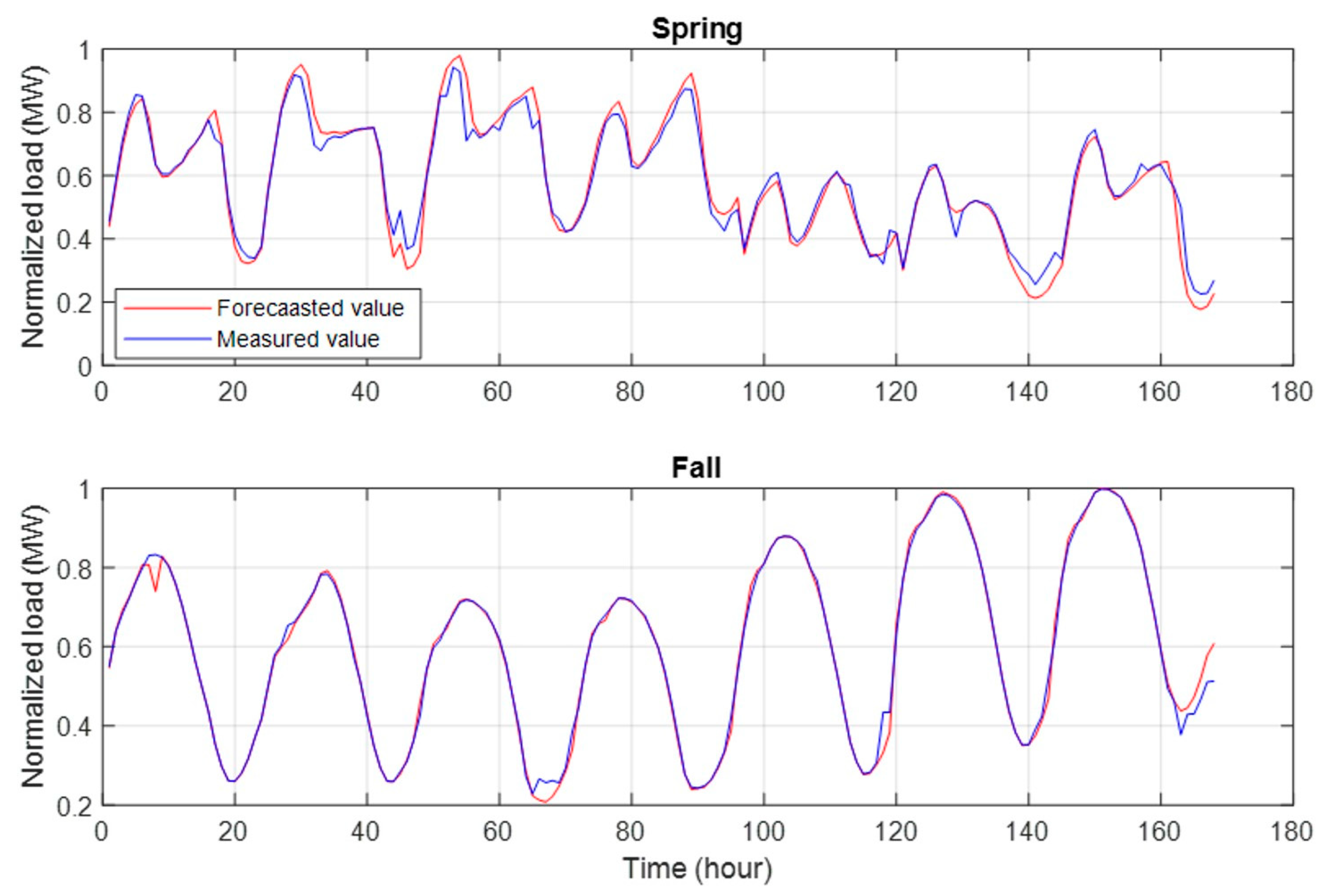
7.2. Load Forecasting Results
8. Conclusions
Funding
Institutional Review Board Statement
Informed Consent Statement
Data Availability Statement
Acknowledgments
Conflicts of Interest
Nomenclature
| ARIMA | Autoregressive integrated moving average | PJM | Pennsylvania-New Jersey-Maryland |
| ML | Machine learning | WT | Wavelet transform |
| GAM | Generalized additive models | DWT | Discrete wavelet transform |
| XGBoost | Extreme gradient boosting | CWT | Continuous wavelet transform |
| STLF | Short-term load forecasting | NLOS | Non-line of sight |
| NN | Neural network | ICA | Imperialist Competitive Algorithm |
| LSTM | Long short-term memory | GA | Genetic Algorithm |
| RNN | Recurrent neural network | MLP-BR | Multilayer Perceptron-Bayesian Regularization |
| CNN | Convolutional neural network | CNN-EA | Cascaded Neural Network-Evolutionary Algorithms |
| EGWO | Enhanced grey wolf optimizer | RMSE | Root mean square error |
| RBF | Radial basis function | MAE | Mean absolute error |
| TEO | Thermal exchange optimization | MAPE | Mean absolute percentage error |
References
- Yu, Z.; Niu, Z.; Tang, W.; Wu, Q. Deep learning for daily peak load forecasting—A novel gated recurrent neural network combining dynamic time warping. IEEE Access 2019, 7, 17184–17194. [Google Scholar] [CrossRef]
- Jacob, M.; Neves, C.; Vukadinović Greetham, D. Forecasting and Assessing Risk of Individual Electricity Peaks; Mathematics of Planet Earth, Springer Briefs in Mathematics of Planet Earth; Springer: Cham, Switzerland, 2020; p. 108. Available online: https://centaur.reading.ac.uk/95824/ (accessed on 1 July 2023).
- Heydari, A.; Nezhad, M.M.; Pirshayan, E.; Garcia, D.A.; Keynia, F.; De Santoli, L. Short-term electricity price and load forecasting in isolated power grids based on composite neural network and gravitational search optimization algorithm. Appl. Energy 2020, 277, 115503. [Google Scholar] [CrossRef]
- Hoseinzadeh, S.; Nastasi, B.; Groppi, D.; Garcia, D.A. Exploring the penetration of renewable energy at increasing the boundaries of the urban energy system—The PRISMI plus toolkit application to Monachil, Spain. Sustain. Energy Technol. Assess. 2022, 54, 102908. [Google Scholar] [CrossRef]
- Hoseinzadeh, S.; Groppi, D.; Sferra, A.S.; Di Matteo, U.; Astiaso Garcia, D. The PRISMI plus toolkit application to a grid-connected mediterranean island. Energies 2022, 15, 8652. [Google Scholar] [CrossRef]
- Almazrouee, A.I.; Almeshal, A.M.; Almutairi, A.S.; Alenezi, M.R.; Alhajeri, S.N. Long-term forecasting of electrical loads in kuwait using prophet and holt–winters models. Appl. Sci. 2020, 10, 5627. [Google Scholar] [CrossRef]
- Khwaja, A.S.; Naeem, M.; Anpalagan, A.; Venetsanopoulos, A.; Venkatesh, B. Improved short-term load forecasting using bagged neural networks. Electr. Power Syst. Res. 2015, 125, 109–115. [Google Scholar] [CrossRef]
- Espinoza, M.; Suykens, J.A.; Belmans, R.; De Moor, B. Electric load forecasting. IEEE Control Syst. Mag. 2007, 27, 43–57. [Google Scholar]
- Heydari, A.; Astiaso Garcia, D.; Keynia, F.; Bisegna, F.; De Santoli, L. Hybrid intelligent strategy for multifactor influenced electrical energy consumption forecasting. Energy Sources Part B Econ. Plan. Policy 2019, 14, 341–358. [Google Scholar] [CrossRef]
- Deng, Z.; Wang, B.; Xu, Y.; Xu, T.; Liu, C.; Zhu, Z. Multi-scale convolutional neural network with time-cognition for multi-step short-term load forecasting. IEEE Access 2019, 7, 88058–88071. [Google Scholar] [CrossRef]
- Saber, A.Y.; Alam, A.R. Short term load forecasting using multiple linear regression for big data. In Proceedings of the 2017 IEEE Symposium Series on Computational Intelligence (SSCI), Honolulu, HI, USA, 27 November–1 December 2017; pp. 1–6. [Google Scholar]
- Zhu, X.; Shen, M. Based on the ARIMA model with grey theory for short term load forecasting model. In Proceedings of the 2012 International Conference on Systems and Informatics (ICSAI2012), Yantai, China, 19–20 May 2012; pp. 564–567. [Google Scholar]
- Christiaanse, W.R. Short-term load forecasting using general exponential smoothing. IEEE Trans. Power Appar. Syst. 1971, 2, 900–911. [Google Scholar] [CrossRef]
- Huang, S.J.; Shih, K.R. Short-term load forecasting via ARMA model identification including non-Gaussian process considerations. IEEE Trans. Power Syst. 2003, 18, 673–679. [Google Scholar] [CrossRef]
- Antoniadis, A.; Brossat, X.; Cugliari, J.; Poggi, J.M. A prediction interval for a function-valued forecast model: Application to load forecasting. Int. J. Forecast. 2016, 32, 939–947. [Google Scholar] [CrossRef]
- Cho, H.; Goude, Y.; Brossat, X.; Yao, Q. Modeling and forecasting daily electricity load curves: A hybrid approach. J. Am. Stat. Assoc. 2013, 108, 7–21. [Google Scholar] [CrossRef]
- Hong, T.; Pinson, P.; Fan, S. Global energy forecasting competition 2012. Int. J. Forecast. 2014, 30, 357–363. [Google Scholar] [CrossRef]
- Lloyd, J.R. GEFCom2012 hierarchical load forecasting: Gradient boosting machines and Gaussian processes. Int. J. Forecast. 2014, 30, 369–374. [Google Scholar] [CrossRef]
- Park, D.C.; El-Sharkawi, M.A.; Marks, R.J.; Atlas, L.E.; Damborg, M.J. Electric load forecasting using an artificial neural network. IEEE Trans. Power Syst. 1991, 6, 442–449. [Google Scholar] [CrossRef]
- Ryu, S.; Noh, J.; Kim, H. Deep neural network based demand side short term load forecasting. Energies 2017, 10, 3. [Google Scholar] [CrossRef]
- Goude, Y.; Nedellec, R.; Kong, N. Local short and middle term electricity load forecasting with semi-parametric additive models. IEEE Trans. Smart Grid 2013, 5, 440–446. [Google Scholar] [CrossRef]
- Wood, S.N.; Goude, Y.; Shaw, S. Generalized additive models for large data sets. J. R. Stat. Soc. Ser. C Appl. Stat. 2015, 64, 139–155. [Google Scholar] [CrossRef]
- Liao, X.; Cao, N.; Li, M.; Kang, X. Research on short-term load forecasting using XGBoost based on similar days. In Proceedings of the 2019 International Conference on Intelligent Transportation, Big Data & Smart City (ICITBS), Changsha, China, 12–13 January 2019; pp. 675–678. [Google Scholar]
- Li, L.; Meinrenken, C.J.; Modi, V.; Culligan, P.J. Short-term apartment-level load forecasting using a modified neural network with selected auto-regressive features. Appl. Energy 2021, 287, 116509. [Google Scholar] [CrossRef]
- Fekri, M.N.; Patel, H.; Grolinger, K.; Sharma, V. Deep learning for load forecasting with smart meter data: Online Adaptive Recurrent Neural Network. Appl. Energy 2021, 282, 116177. [Google Scholar] [CrossRef]
- Jalali, S.M.J.; Ahmadian, S.; Khosravi, A.; Shafie-khah, M.; Nahavandi, S.; Catalão, J.P. A novel evolutionary-based deep convolutional neural network model for intelligent load forecasting. IEEE Trans. Ind. Inform. 2021, 17, 8243–8253. [Google Scholar] [CrossRef]
- Chitalia, G.; Pipattanasomporn, M.; Garg, V.; Rahman, S. Robust short-term electrical load forecasting framework for commercial buildings using deep recurrent neural networks. Appl. Energy 2020, 278, 115410. [Google Scholar] [CrossRef]
- Mallat, S.G. A Theory for Multiresolution Signal Decomposition: The Wavelet Representation. IEEE Trans. Pattern Anal. Mach. Intell. 1989, 11, 674–693. [Google Scholar] [CrossRef]
- Reis, A.J.R.; Alves da Silva, A.P. Feature Extraction via Multiresolution Analysis for Short-Term Load Forecasting. IEEE Trans. Power Syst. 2005, 20, 189–198. [Google Scholar] [CrossRef]
- Kaveh, A.; Dadras, A. Advances in Engineering Software A novel meta-heuristic optimization algorithm: Thermal exchange optimization. Adv. Eng. Softw. 2017, 110, 69–84. [Google Scholar] [CrossRef]
- Broomhead, D.S.; Lowe, D. Radial basis functions, multi-variable functional interpolation and adaptive networks. Complex Syst. 1988, 2, 321–355. [Google Scholar]
- PJM Web Site. Available online: http://www.pjm.com (accessed on 1 July 2023).
- Amjady, N. Short-Term Bus Load Forecasting of Power Systems by a New Hybrid Method. IEEE Trans. Power Syst. 2007, 22, 333–341. [Google Scholar] [CrossRef]
- Catalão, J.P.D.S.; Mariano, S.J.P.S.; Mendes, V.M.F.; Ferreira, L.A.F.M. Short-term electricity prices forecasting in a competitive market: A neural network approach. Electr. Power Syst. Res. 2007, 77, 1297–1304. [Google Scholar] [CrossRef]
- Amjady, N.; Keynia, F. Day ahead price forecasting of electricity markets by a mixed data model and hybrid forecast method. Int. J. Electr. Power Energy Syst. 2008, 30, 533–546. [Google Scholar] [CrossRef]


| Time | Models | Case I | Case II | ||||
|---|---|---|---|---|---|---|---|
| WT-RBF-GA | WT-RBF-ICA | WT-RBF-TEO | WT-RBF-GA | WT-RBF-ICA | WT-RBF-TEO | ||
| Spring | RMSE | 0.044 | 0.033 | 0.020 | 0.121 | 0.069 | 0.017 |
| MAE | 0.028 | 0.022 | 0.007 | 0.100 | 0.055 | 0.016 | |
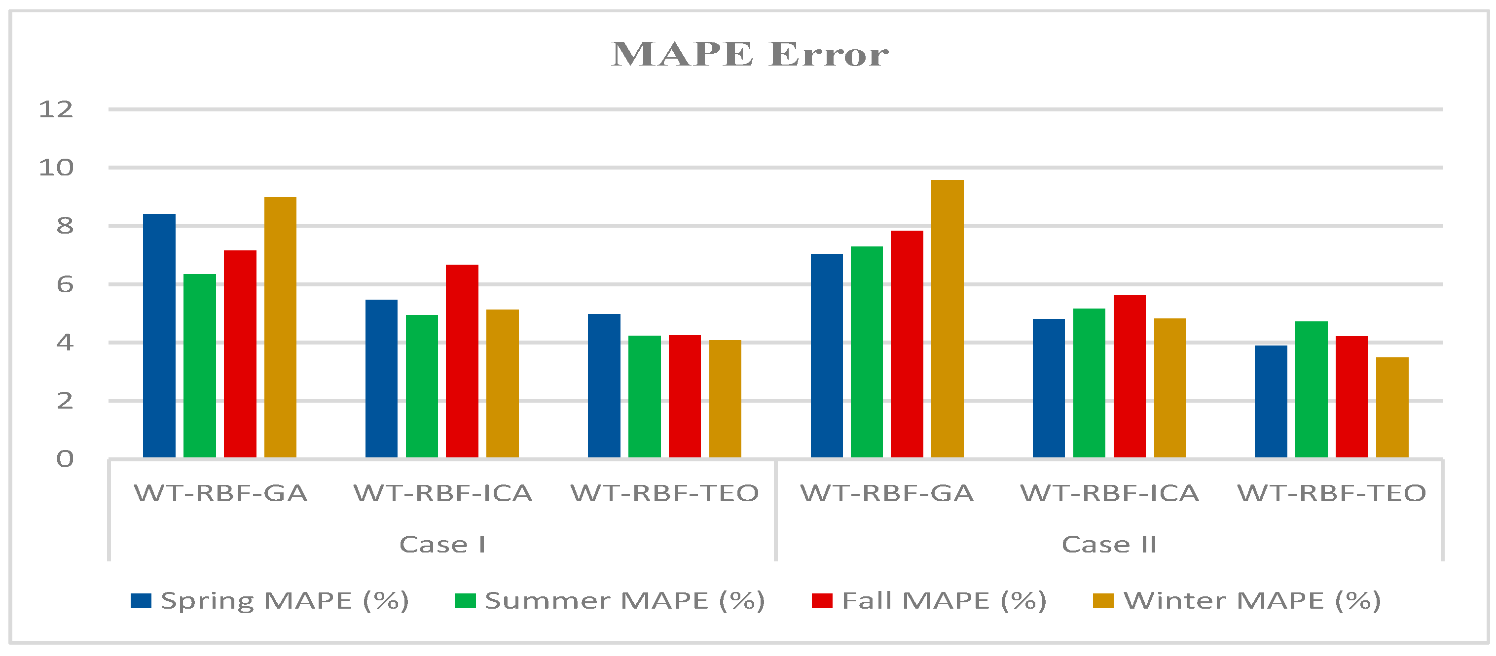
| MAPE (%) | 8.415 | 5.466 | 4.979 | 7.034 | 4.810 | 3.899 | |
| Summer | RMSE | 0.074 | 0.055 | 0.020 | 0.055 | 0.044 | 0.017 |
| MAE | 0.061 | 0.045 | 0.010 | 0.043 | 0.033 | 0.007 | |
| MAPE (%) | 6.348 | 4.952 | 4.226 | 7.292 | 5.162 | 4.717 | |
| Fall | RMSE | 0.027 | 0.020 | 0.006 | 0.097 | 0.071 | 0.014 |
| MAE | 0.023 | 0.017 | 0.004 | 0.080 | 0.052 | 0.020 | |
| MAPE (%) | 7.156 | 6.657 | 4.255 | 7.844 | 5.618 | 4.212 | |
| Winter | RMSE | 0.073 | 0.070 | 0.037 | 0.046 | 0.035 | 0.006 |
| MAE | 0.056 | 0.049 | 0.023 | 0.038 | 0.028 | 0.004 | |
| MAPE (%) | 8.994 | 5.127 | 4.087 | 9.584 | 4.821 | 3.492 | |
| Seasons | MLP-BR | NN | CNN-EA | Proposed Model |
|---|---|---|---|---|
| Winter | 13.22 | 9.82 | 4.44 | 3.49 |
| Spring | 12.92 | 8.87 | 4.31 | 3.90 |
| Summer | 11.98 | 10.43 | 4.78 | 4.71 |
| Fall | 12.24 | 9.54 | 4.75 | 4.21 |
| Average | 12.24 | 9.54 | 4.75 | 4.21 |
Disclaimer/Publisher’s Note: The statements, opinions and data contained in all publications are solely those of the individual author(s) and contributor(s) and not of MDPI and/or the editor(s). MDPI and/or the editor(s) disclaim responsibility for any injury to people or property resulting from any ideas, methods, instructions or products referred to in the content. |
© 2023 by the author. Licensee MDPI, Basel, Switzerland. This article is an open access article distributed under the terms and conditions of the Creative Commons Attribution (CC BY) license (https://creativecommons.org/licenses/by/4.0/).
Share and Cite
Khan, S. Short-Term Electricity Load Forecasting Using a New Intelligence-Based Application. Sustainability 2023, 15, 12311. https://doi.org/10.3390/su151612311
Khan S. Short-Term Electricity Load Forecasting Using a New Intelligence-Based Application. Sustainability. 2023; 15(16):12311. https://doi.org/10.3390/su151612311
Chicago/Turabian StyleKhan, Salahuddin. 2023. "Short-Term Electricity Load Forecasting Using a New Intelligence-Based Application" Sustainability 15, no. 16: 12311. https://doi.org/10.3390/su151612311
APA StyleKhan, S. (2023). Short-Term Electricity Load Forecasting Using a New Intelligence-Based Application. Sustainability, 15(16), 12311. https://doi.org/10.3390/su151612311