Doppler Sodar Measured Winds and Sea Breeze Intrusions over Gadanki (13.5° N, 79.2° E), India

Abstract

Doppler sodar measurements were made at the tropical Indian station, i.e., Gadanki (13.5° N, 79. 2° E). According to wind climatologies, the wind pattern changes from month to month. In July and August, the predominant wind direction during the monsoon season was the southwest. In September, it was the northwest and south. While the winds in November came from the northeast, they came from the northwest and southwest in October. The winds in December were out of the southeast. The diurnal cycle of winds at 60-m above the ground was visible, with disturbed wind directions in September and October. This may be connected to the Indian subcontinent’s southeastern monsoon recession. To better understand the monsoon circulation on a monthly basis, the present work is innovative in that it uses high-resolution winds measured using the Doppler sodar at the atmospheric boundary layer. The convergence of a sea breeze and the background wind might result in a sudden change in wind direction, and forecasting such a chaotic atmospheric event is crucial in the aviation sector. As a result, the wind shear that is produced may pose a serious threat to airplanes that are landing. In the current study, we present a few cases of sea breeze intrusions. The physics underlying these intrusions may help modelers better understand these chaotic wind structures and use them as inputs in their models. Based on surface-based atmospheric characteristics, there have been two reports of deep sea breeze intrusions that we report in this research. The sea breeze days were marked by substantial (moderate) drops in temperature (dewpoint temperatures) and increased wind speed and relative humidity. The India Meteorological Department (IMD) rainfall data showed a rise in precipitation over this location on 23 July (4.8 mm) and 24 July (9.5 mm) when sea breeze intrusions over Gadanki were noticed. Sea breeze intrusions could have brought precipitation (intrusion-laden precipitation) to this area due to conducive meteorological conditions. A simple schematic model is proposed through a diagrammatic illustration that explains how a sea breeze triggers precipitation over adjacent locations to the seacoast. The skew-T log-P diagrams have been drawn using the balloon-borne radiosonde measured atmospheric data over Chennai (a nearby location to Gadanki) to examine the thermodynamic parameters to gain insights into the underlying mechanisms and meteorological conditions during sea breeze intrusion events. It is found that the convective available potential energy (CAPE), which is presented as a thermos diagram, was associated with large values on 23 July and 24 July (898 J/kg and 1250 J/kg), which could have triggered thunderstorms over Chennai.

1. Introduction

Profile measurements of low-level wind are crucial for studies of the atmospheric boundary layer, land–sea breeze circulations, surface-based temperature inversion, pollution transport and dispersion, wind energy application, aviation meteorological factors, etc. [1,2,3,4]. Acoustic remote sensing tools like sodar (sound detection and ranging) and optical instruments such as wind LIDAR (LIght Detection and Ranging) allow researchers to investigate the wind profiles and their detailed dynamics with high spatial and temporal resolution. Wind studies over forests, complex topography, and hills are relatively rare [5,6,7,8] compared to planes and homogenous surfaces.

Crescenti [9] documented two decades of the results obtained from various sodar experiments conducted worldwide. For example, Lokoshchenko and Yavlyaeva [10], using a Doppler sodar over Moscow from 2004 to 2008, found that the strongest winds were identified in autumn and winter, while the weakest were detected in spring and summer. Two similar Doppler sodars were operated at both valley and flatland sites in Austria from November 2006 to June 2007 (from winter to spring seasons) under quite different ambient conditions and found that the atmosphere in the valley was stable, whereas the flatland station had relatively higher average wind speeds, temperatures, and turbulence [11].

Egger et al. [12] used data from pilot balloons in September and October 1998 to analyze the diurnal wind system of the Kali Gandaki Valley in Nepal. They found an up-valley wind layer of 1–2 km depth during the day and a weak drainage flow of 1 km depth at night. Stewart et al. [13] investigated the diurnal evolution and consistency of thermally induced winds in four regions of the US Intermountain West using surface measurements from the MesoWest cooperative networks. They found a high level of day-to-day wind consistency at night and a low level of wind consistency during transition periods from up-valley to down-valley winds.

Zhong et al. [14] used data from 22 radar wind profiler/radio acoustic sounding devices to create climatology of mean winds in the Central Valley of California throughout the summer season. Within the lowest 300 m, they found a low-level wind maximum with wind speeds up to 10 m s⁻¹. Other studies that use data to provide the structure of diurnal valley winds over complex topography are, for example, [2,12,15,16,17]. Because wind climatologies over typical complex terrains are usually distinctly diverse and largely dependent on climatic and local conditions [18], it is necessary to sample a set of different terrains to advance our understanding. This motivated us to examine the diurnal winds over Gadanki, a typical complex topography station in southern India. Although various studies have used Doppler sodar to analyze wind climatologies in the atmospheric boundary layer [3,19,20,21], systematic investigations in complex terrain are rare. Importantly, because the present station (Gadanki) is also located in complex topography, where the Indian MST (Mesosphere, Stratosphere, and Troposphere) radar is located, this study assumes significance in understanding typical wind climatologies.

Further, the sea breeze circulation or SBC, which is a local wind system characterized by a flow from sea to land during the day, can influence the weather and climatic dynamics of coastal areas and their nearby locations from polar regions to the equator [22]. SBC arises from the differential heating of land and water [23] when relatively cloud-free skies exist [22]. Sea breezes can even alter near-surface wind direction and magnitude, temperature, and precipitation patterns during the warm season [23,24,25]. Many of the studies on the sea breeze have used an automatic meteorological station [26,27], radar and/or satellite data [28], and Doppler sodar [2,29].

Sea breezes have traveled up to 400 km inland in northern Australia [30] but just 75 km over India’s west coast [31]. It was argued that sea breezes associated with intense precipitation develop to a greater vertical extent closer to the coastline and penetrate further inland than sea breeze days with no precipitation [32]. Although the fundamental understanding of sea breeze circulations has been developed, it can be difficult to generalize single observational studies. In a broader sense, generalizing previous studies is particularly challenging because properties of local atmospheric conditions can interact to affect sea breeze characteristics in nonlinear ways [33,34].

On the application side, the studies of sea breeze intrusions assume great significance as far as the aviation industry is concerned. For example, the convergence of a sea breeze and the background wind can bring about a sudden change in wind direction. Those eventualities may, sometimes, be considered as wind shear by the landing aircraft [35]. It is an important task for the airport authorities to forecast the occurrence of sea breeze events (timing, strength, and change of wind direction) accurately. To model sea breeze intrusions, several high-resolution models have been proposed [36,37], but no consensus has yet been achieved. One school of thought claimed that the Weather Research and Forecasting (WRF) model was unable to reproduce the sea breeze development [36], while other studies reported positive results [37].

In these circumstances, case studies of sea breeze circulations may produce new observational findings to deepen our comprehension. The present research may further assist the modelers in digging out the physics underlying these significant chaotic weather events. Therefore, a few cases of sea breeze intrusions in July 2015 over Gadanki were reported, and the physics behind these studies could be useful as inputs to the modelers.

This research paper is arranged as follows: Section 2 provides information on the datasets used in this work, and a detailed data analysis methodology is also discussed in the same section. Section 3 presents the study site in terms of elevation, pictures taken using a high-resolution camera, and a topography map. Section 4 contains observational results and a discussion, including wind speed concerning wind directions, diurnal variations of various wind parameters at different heights, and a few cases of sea breeze intrusions. Through a diagrammatic illustration, a simple schematic model is proposed to describe how sea breezes cause precipitation to occur over areas near the seacoast in Section 4. The summary and future scope of this research are included in Section 5.

2. Methodology

2.1. Doppler Sodar Data and Analysis

We used measurements (July–December 2015) from the Doppler sodar installed at the National Atmospheric Research Laboratory (NARL), Gadanki, India. The NARL Doppler sodar is a phased-array antenna system of 8 × 8 arrays of piezoelectric transducers. Three elements were removed from each corner of the antenna system to create a circular array pattern with a side lobe suppression of 17 dB. The antenna is at 70°, and the reflector is at 35° about the ground plane providing transmission and reception in reflected mode.

The sodar can transmit multiple frequencies (between 1600 and 2500 Hz) with a maximum of up to 10 in sequence. However, for the present study, the sodar operated at 1.8 KHz with a peak power of 100 W. The three components of wind velocities (zonal, meridional, and vertical) and other scattering characteristics (power, signal-to-noise ratio, etc.) are measured using beams tilted from zenith in the east and north directions between 30 m and 1500 m in height. After passing the quality check, the radial wind velocities were utilized to calculate the zonal, meridional, and vertical components of wind.

For the first time in the data processing, the received signal was digitized and subjected to the fast Fourier transform (FFT) process for online computation of Doppler spectra for each range bin. The three low-order spectral moments are computed through numerical integration [38]. The three moments represent the spectrum’s signal strength, weighted mean Doppler shift, and half-width parameters.

The pulse width and interpulse period can be programmed to get a range resolution between 10 and 200 m for an altitude coverage of 1500 m. Nevertheless, the three components of wind velocities and other scattering characteristics (power, signal-to-noise ratio, etc.) are measured using beams tilted from zenith in the east and north directions between 30 m and 1500 m in height.

The sodar wind measurements were recorded at a temporal resolution of 27 s, and we further averaged the winds every 30 min, which enabled us to eliminate the data artifacts. The sodar estimated horizontal wind speed has an uncertainty of 0.1 m s^−1, and the wind direction has an uncertainty of 3° [39]. The theoretical foundation and practical application of the NARL sodar technique are in [39].

The major technical specifications are listed in

Table 1. Technical specification of the NARL sodar system [39].

Parameter	Specification
Operating frequency	1.8 kHz
Peak power	100 W
Antenna array	1 m × 1 m
Pulse width	180 ms
Interpulse period	9 × 106 μs
No. of coherent integrations	1
No. of incoherent integrations	1
No. of FFT points	4096
Beam width	4°
Range resolution	30 m
Beam directions	North 16, Zenith, East 16

.

2.2. A Co-Located Weather Station, IMD Rain, and ERA5 Model Datasets

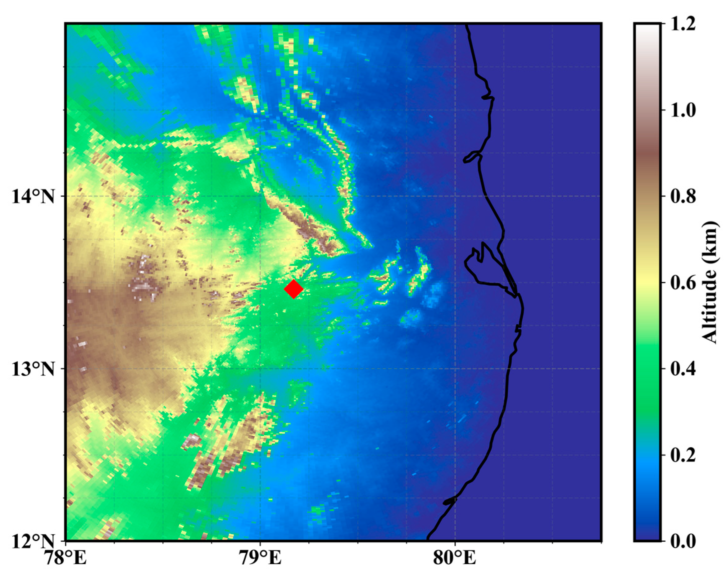
To verify the sea breeze intrusions over Gadanki, we used a surface-based and co-located weather station to measure atmospheric parameters, including temperature, wind speed, dewpoint temperature, and relative humidity. The diurnal variations of the atmospheric parameters for three continuous days (23–25 July 2015) are presented to verify the sea breeze intrusions over Gadanki.

The India Meteorological Department (IMD) rain data is also used to determine precipitation (mm) in response to the sea breeze intrusions over Gadanki, India. We also used the ERA5 (~30 km grid spacing) dataset produced by the European Centre for Medium-Range Weather Forecasts (ECMWF) to examine the synoptic wind condition and temperature distribution. ERA5 data details are available at https://www.cds.climate.copernicus.eu (accessed on 4 May 2023).

3. Site Description

Gadanki is a tropical rural station, which is located over the southern peninsula and is 80 km away from India’s east coast. Figure 1 depicts the elevation map of the sodar site and nearby locations, along with the Bay of Bengal (BoB) coast on the east side. The map used in Figure 1 is generated using Shuttle Radar Topography Mission (SRTM) Version 3.0 Global one arc second data in similar lines to Farr et al., 2007 [40]. Figure 2a shows the NARL sodar (heavy white dot shown with a black arrow) in the Indian MST radar (see the erected antennae in the background) location (which was taken using a high-resolution camera), while Figure 2b shows the topography map. It may be worth mentioning here that the XY plane is tilted at a 40-degree angle to obtain a clear location of the site.

It is situated at 370 m above sea level and is surrounded by hillocks that, in a one-kilometer radius, range in height from 200 to 300 m and, in a ten-kilometer radius, vary in vegetation. The terrain’s elevation is unevenly distributed around Gadanki: modest hills of 200 m can be found to the east and west. There are several ridges and small hills of different heights between these two places, as can be seen in Figure 2a.

4. Results and Discussion

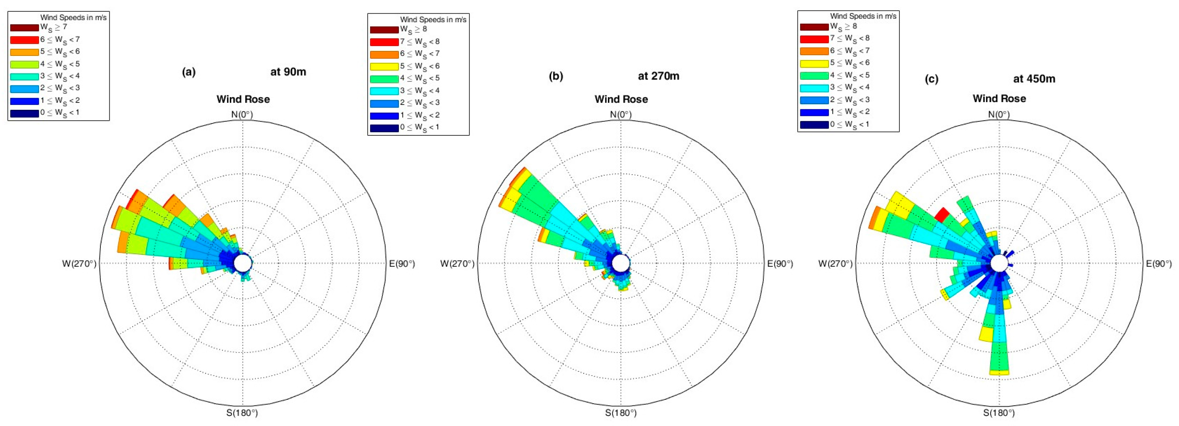
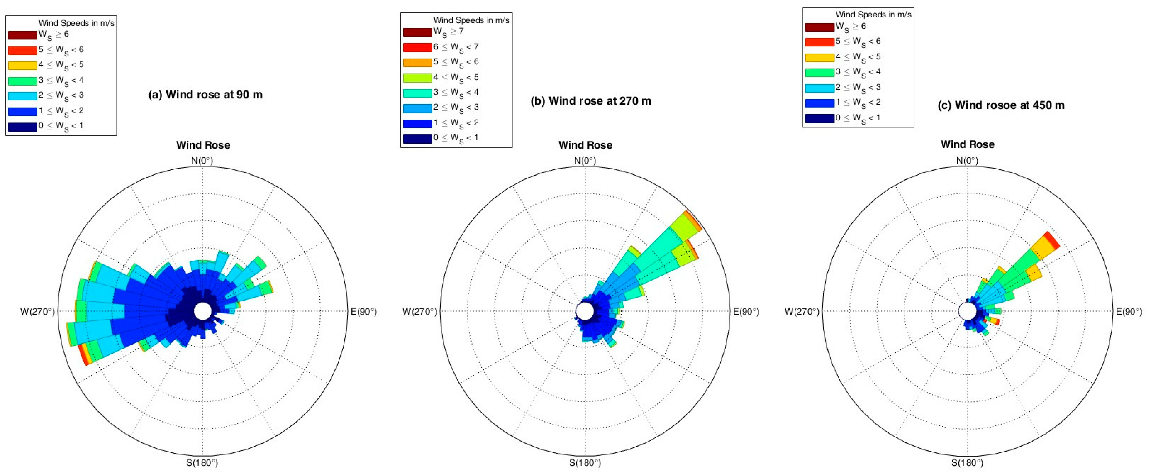
4.1. Monthly Variation of Wind Speeds and Directions

The hourly averages of wind rose diagrams that depict the prevailing winds over Gadanki, India, at three different altitudes have been constructed to examine the dynamic state of the overlying atmosphere. Figure 3 illustrates hourly averages in the month of July 2015 wind roses over Gadanki at various altitudes, including 90 m, 270 m, and 450 m in four 90° wind direction bands. The dominant winds were blown between the southwest (SW) and northwest (NW) directions at 90 m (Figure 3a). At 270 m and 450 m altitudes (Figure 3b,c), the prevailing winds were SW and NW, but the dominant winds were associated with NW. Maximum wind speeds at 90 m, 270 m, and 450 m are 7 m/s, 7 m/s, and 8 m/s, respectively.

Figure 4 presents the wind roses (hourly averages) in the month of August 2015. It can be noted that NW winds were dominant, with a few exceptions. For example, although winds at 90 m (Figure 4a) and 270 m (Figure 4b) are generally NW, winds at 450 m (Figure 4c) are mostly northeast (NE) as well as southward. The maximum velocity of winds at 90 m, 270 m, and 450 m are estimated to be 7 m/s, 7 m/s, and 8 m/s, respectively.

September 2015 wind roses at various altitudes are presented in Figure 5. Figure 5a shows that wind roses (hourly averages) at 90 m were blown between NW and SW directions. However, the winds at 270 and 450 m (Figure 5b,c) have reached all directions, but they predominantly emanated from the NW. The maximum winds at 90 m, 270 m, and 450 m are 7 m/s, 7 m/s, and 8 m/s, respectively.

Figure 6 shows the prevailing winds in October 2015 at various altitudes. The prevailing winds were densely distributed at 90 m (Figure 6a), 270 m (Figure 6b), and 450 m (Figure 6c), despite the prevailing winds at 270 m showing northeast (NE) directions. Maximum wind speeds were 7 m/s, 7 m/s, and 6 m/s, respectively. This suggests that winds were of weaker magnitudes than in July, August, and September.

December month wind roses at different altitudes, including 90 m, 270 m, and 450 m, can be seen in Figure 7. The winds at 90 m (Figure 7a) moved from SW to NE directions but winds at 270 and 450 m (Figure 7b,c) had, as expected, moved in NE directions. At 90, 270, and 450 m, the maximum wind magnitudes were 6 m/s, 7 m/s, and 6 m/s, respectively.

Piringer and Kaiser [11] found that winds were funneled along the valley axis at 100 m with a 1290 MHz sodar/RASS (manufactured by Metek Company, Elmshorn, Germany), which was located in an industrially used narrow valley in central Austria. The channeling effect was not detected at the present station, which contradicts [11]. On the other hand, the winds at 270 and 450 m were likely caused by pressure gradient forces (PGFs) since the lower elevation of the hills surrounding the NARL observatory could not affect prevailing winds at these altitudes.

The unevenly distributed terrain surrounding the present observation station (NARL) may have contributed to the wide distribution of the prevailing winds at 90 m in July, October, November (not shown here), and December, as it is commonly accepted that winds in complex terrain can be more inhomogeneous [41]. Given that terrain roughness and complexity affect wind flow in the direction of approach, the prevailing wind would be expected to change under the influence of hills around the study site.

The possible reasons why channeling was not observed at 60 m above the ground surface could be: The present study location is neither a narrow nor a deep valley (see, Figure 2a), as against the [11] observations conducted in an extremely narrow and deep valley, that might not allow a channeling effect. Secondly, winds are sensitive to the level of overlying turbulence, which again depends on the surface roughness, slope condition, and the topographic features [42]. Because the topography of the present location is complex and it looks as if it is scattered, and it is also covered with the presence of small hills here and there, the channeling effect was not observed, or the impact of the valley on wind flow was not as significant as expected. Rather, a disturbed wind pattern was observed at 60 m above the ground surface.

The present observations support the earlier results of wind direction at various altitudes in different months [43]. For instance, since June–September coincides with the SW monsoon, the prevailing winds in July, August, and September were almost restricted to the northwest and southwest, indicating the active phase of the monsoon. In September, the prevailing winds at 270 and 450 m are irregular in structure, which can be attributed to the monsoon withdrawal period [43]. As October, November, and December are part of the post-monsoon or NE monsoon period, most of the wind directions were north or east, which is again similar to the earlier studies. Other interesting coincidences that corroborate the earlier studies include relatively lower wind speeds during the post-monsoon period compared to the monsoon period.

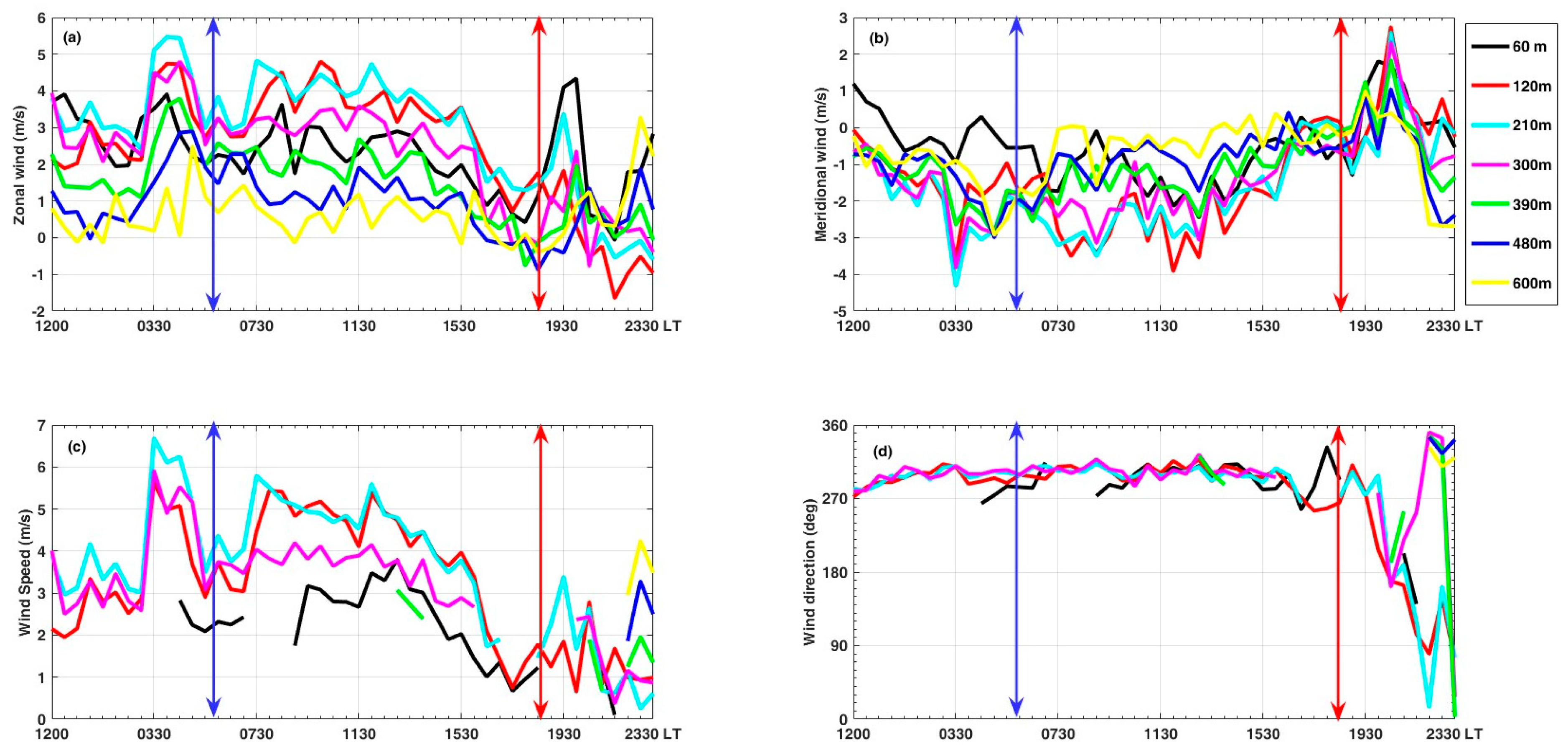
4.2. Diurnal Variations of Wind Parameters in Different Months

Sodar observations are commonly matched with other sodar systems and cup/vane anemometer data to estimate mean wind speed and direction [39,42]. The correlation between the NARL sodar and a co-located sodar (Scintec model MFAS64) observations of wind speed and direction and horizontal velocities is greater than 0.8 [39], demonstrating good agreement and a very low level of uncertainty for the data retrieved from the NARL sodar.

Figure 8 shows the daily course of zonal and meridional winds, wind speed, and direction in July 2015 at different altitudes. Figure 8a demonstrates that zonal winds exhibit a distinct diurnal variation. Zonal winds, for example, do not just peak at midday but also during the early morning hours (between 03:00 and 04:00 AM) as well as during post-evening time, i.e., at 07:30 PM. Peak magnitudes during the early morning hours have been observed from 120 to 390 m above ground. In meridional winds, there were no distinct diurnal fluctuations (Figure 8b), nor great wind magnitudes were observed. Nevertheless, the winds at 60 m above ground level (wind at 60 m altitude) revealed a distinct diurnal variation in its zonal and meridional components. Wind speed (Figure 8c) also showed similar trends in similar lines with zonal winds. From early morning to late evening, the wind direction (Figure 8d) was NW before suddenly turning to the northward direction.

The zonal wind, Figure 9a, showed distinct diurnal variations when compared to its meridional counterparts in August 2015, but no significant morning peak was observed. Meridional winds (Figure 9b) did not show any significant diurnal variations, and wind speeds (Figure 9c) showed prominent diurnal variation, as did zonal winds, although the winds at 60 m above ground level did not show any significant diurnal variation.

The diurnal variation of zonal (meridional) winds is presented in Figure 10a (Figure 10b), and wind speeds and direction were evaluated in Figure 10c,d in September 2015. The westward wind had diurnal dominance at all altitudes, but the winds at 60 m above ground level had an eastward component, and the meridional winds had moderate diurnal fluctuations. On the other hand, wind speeds with lower magnitudes and wind directions were highly disruptive.

In October 2015, diurnal dominance in both meridional and zonal winds (Figure 11a,b) could be seen at all altitudes, but the zonal component of winds at 60 m above ground level showed a significant diurnal variation. Wind speeds (Figure 11c) associated with lower magnitudes and wind directions (Figure 11d) showed a disturbing nature.

In November 2015, diurnal dominance in both zonal (Figure 12a) and meridional (Figure 12b) winds was evident at all altitudes, but both the zonal and meridional components of the winds at 60 m above ground level showed a significant diurnal variation. On the other hand, wind speeds (Figure 12c) are associated with smaller magnitudes, but a distinct diurnal variation could be seen. Wind directions (Figure 12d) are NE, except for those at 90, 120, and 210 m.

Figure 13a shows the diurnal variation of zonal, and Figure 13b shows the diurnal variation of meridional winds in December 2015. Figure 13c,d shows the diurnal variation of wind speed and wind direction. The diurnal influence in both meridional and zonal winds could be observed at all altitudes, but the zonal and meridional components of winds at 60 m above ground level showed a significant diurnal variation. Diurnal variations in wind speed were also evident, with winds turning in the NE direction.

The diurnal variations of zonal and meridional winds, wind speeds, and directions show interesting features, including (a) Larger magnitudes associated with zonal winds than meridional winds, (b) Distinct diurnal variation in zonal winds and wind speeds, (c) Highly disturbed nature of wind directions in September and October, and (d) An early morning peak in the zonal wind in few months.

Zonal winds are winds circulating at the same latitude circles (between east and west directions or between west and east directions), parallel to the equator, thermalizing the atmosphere longitudinally [44] once thermal gradient forces (TGFs) exist between day and the nightside sectors. On the other hand, meridional winds circulate at the same longitudinal circles (meridian), perpendicular to the equator, thermalizing the atmosphere latitudinally once TGFs exist between two different seasons. Consequently, meridional winds show lesser wind magnitudes than zonal winds.

When it comes to diurnal changes in zonal winds and wind speeds, it is well known that near-surface winds over land have a distinct diurnal cycle under clear sky conditions, which is linked to the diurnal cycle in near-surface stratification [45,46,47]. Therefore, the near-surface winds of this study follow similar trends to the earlier studies. In addition, large changes in diurnal wind variations are observed under typical meteorological conditions. These diurnal processes are largely governed by the diurnal cycle of solar radiation (so-called thermally driven winds) [48]. It is also widely acknowledged that diurnal winds change direction twice a day [12,49].

During the well-mixed conditions around noon, wind speeds increase steadily with height throughout the whole heights investigated. The zonal wind component is the largest contributor to the total wind speed, and as a result, their profiles are similar in shape [50]. The highly disturbing nature of wind directions in September and October can be attributed to the withdrawal period of the SE monsoon over the Indian region.

In July, the early morning peak at all altitudes may be due to the nighttime low-level jet (NLJ) [51]. Low-level jets, often known as LLJs, are a broad category of wind characteristics that are present over almost every continent on Earth [52,53]. Wind maxima near the ground may occur at night under clear skies and mild synoptic winds; this phenomenon is known as nocturnal LLJ (NLLJ). This nocturnal LLJ typically resides between 500 m and 700 m above the ground at night [54]. The monsoon month of July is when the LLJ is most regularly spotted in the area with a cross-equatorial circulation flowing from the southern Indian Ocean to the center of the Arabian Sea [55]. This is one of the synoptic elements of the Indian summer monsoon and provides a large moisture supply over land regions, fueling convection [56].

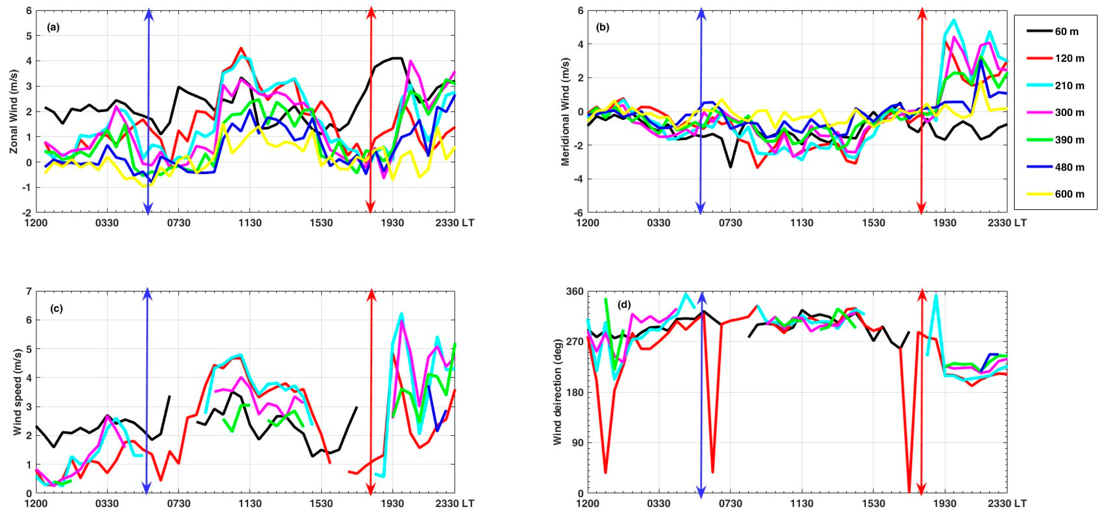
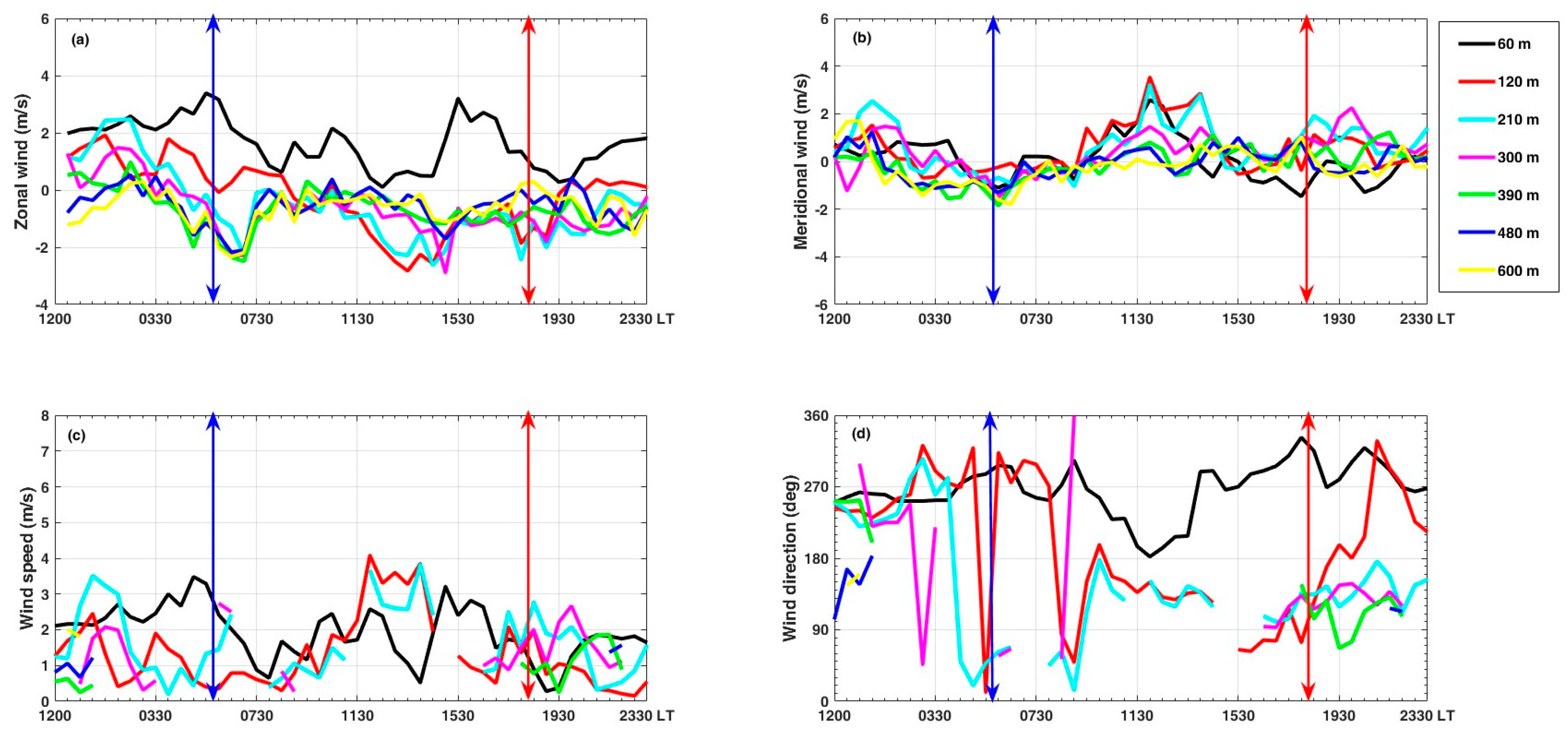
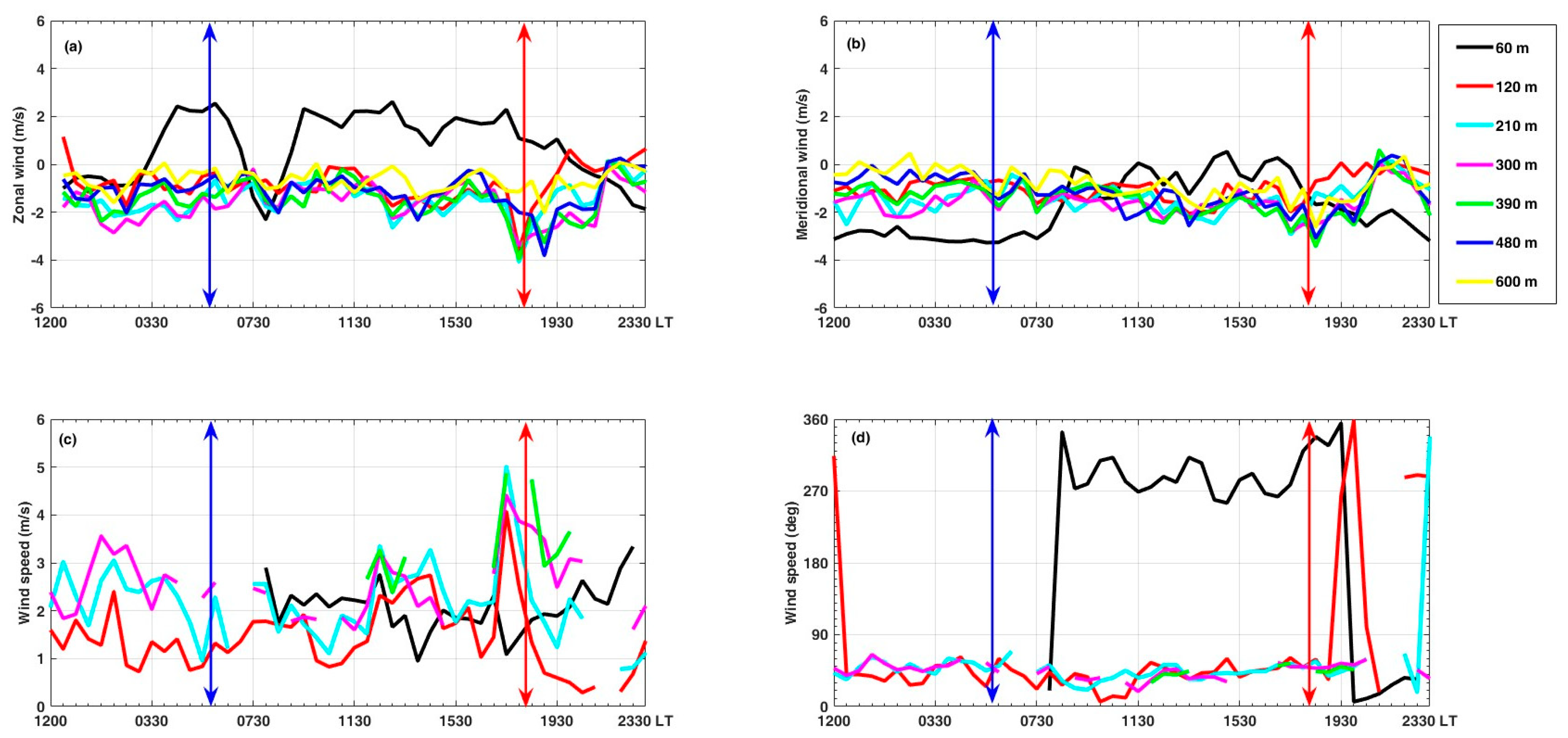
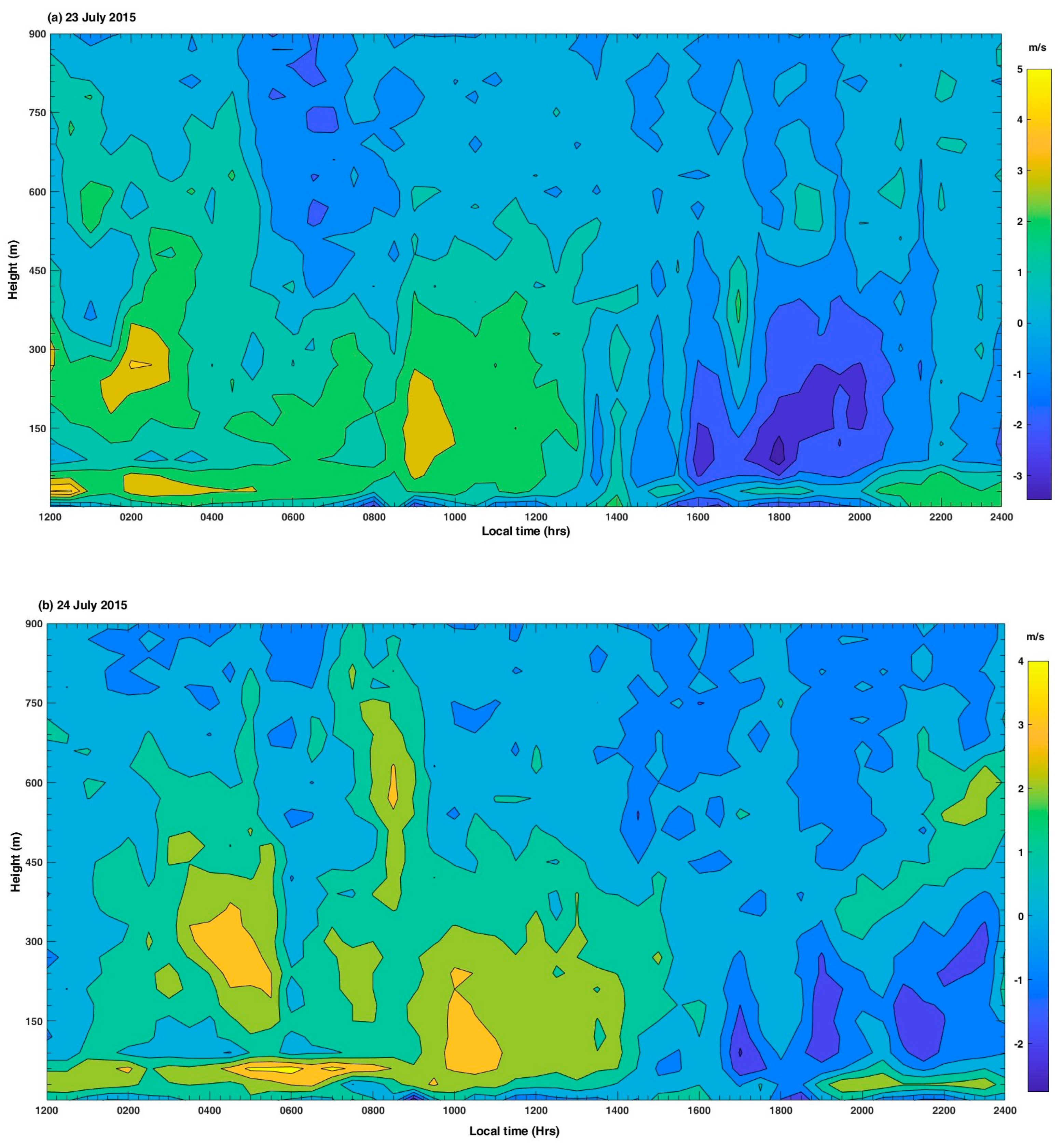
4.3. A Few Cases of Sea Breeze Intrusions

Sea breezes are known to influence the local wind velocity and air quality [24,57] and convective activity [31,58,59,60]. Most importantly, sea breezes, in special circumstances, are a great hurdle to the aviation industry. For example, the convergence of sea breeze and background wind takes place, oftentimes, which results in the formation of wind shear, which is also known as wind gradient. As is well known, wind shears are a major hazard, particularly when an airplane is operating at low levels.

We quantitatively identified sea breeze intrusions on 23 and 24 July 2015 over Gadanki using Doppler sodar observations. We have considered co-located surface-based (an automatic weather station) observations to verify the presence of sea breeze intrusions. In addition, ERA5 data (winds and temperature) are also considered to understand the background synoptic weather conditions.

Synoptic scale background winds play a significant role in the development and evolution of sea breeze intrusions [57,61,62]. Therefore, the studies regarding the interaction between synoptic-scale winds and low-level flows will always assume a great significance that needs to be understood further over different terrains by verifying many databases. In addition, the lower atmospheric layer (from 700 mb to 1000 mb) has an important control on diurnal sea breeze activity [63,64].

Figure 14a shows the diurnal variation of zonal winds on 23 July 2015. A strong sea breeze formed by 1545 local time, LT (Local Time, LT = Universal Time + 0530 h) and lasted until 2200 LT. The airflow was moderate initially but intensified around 1715 LT, and such intensification continued till 2200 LT. After sunset, stability started increasing, the breeze’s height gradually decreased, and such a decrease was predominant by 2130 LT. On the whole, the height of the sea breeze was around 50 m (1530 LT) and reached as high as 500 m.

Figure 14b presents another sea breeze case observed on 24 July 2015. It started at around 1640 LT and continued till around 2400 LT and the height of the sea breeze decreased gradually, in similar lines to the sea breeze intrusion observed on 23 July. We also present a non-sea breeze day observed on 25 July 2015 (Figure 14c). It is quite clear from Figure 14a that wind direction was westward during nighttime hours, with magnitudes higher than 4 m/s.

Figure 15a shows diurnal temperature and wind speed, while Figure 15b shows relative humidity and dewpoint temperature variations from 23 July to 25 July 2015. It may be worth mentioning here that the dew point temperature is the temperature at which air gets completely saturated with water vapor, which causes dew, fog, or clouds to form. The sea breeze timings are marked in Figure 15 (Figure 15a,b) with a double arrow symbol, and the details are provided in Figure captions.

Wind speed, in general, observed during daytime should be higher than the wind speed observed during nighttime due to mixing processes. On 23 July 2015, the wind speed was 2 m/s during the afternoon; it was high at about 3 m/s during the sea breeze event period, i.e., from around 1600 to 2000 LT. The diurnal variations of the temperature on the same date showed a significant decrease from an average of 28 °C to a mere 23 °C from 1545 LT onwards and till around 2200 LT, while a huge increase (from 81% to 99%) in relative humidity (RH) value could also be seen on 23 July 2015. It is also obvious that moderate decreases in dewpoint temperatures were witnessed when sea breeze intrusions were observed.

The wind speed, temperature, and relative humidity on 24 July also showed trends near that of 23 July. For instance, the diurnal variation of temperature showed magnitudes from around 25 °C to a mere 23 °C (1600 LT to 0200 LT). As a result, it had a lower temperature than average, although wind speeds had peaks, one at 1800 LT and another at 2200 LT. On the other hand, relative humidity magnitudes attain greater values during the sea breeze times (96% at 1515 LT and 91% at 2100 LT). In contrast to the changes seen on 23 and 24 July 2015 (sea breeze days), 25 July 2015 (a non-sea breeze day) did not demonstrate any notable changes in diurnal variations of temperature decline, rise in wind speeds, and sudden shift in relative humidity.

ERA5 zonal velocity data are analyzed to understand the sea breeze circulations over Gadanki. Figure 16 shows ERA5 zonal velocity daily data (1.5° × 1.5° grid) at 950 hPa level for 1330 (Figure 16a), 1530 (Figure 16b), 1730 (Figure 16c), and 1930 (Figure 16d) LT on 23 July 2015. Background wind vector (green and yellow contours) is superimposed on the zonal wind component (black arrows) to show the total wind circulations all over Gadanki and nearby regions, while heavy black lines indicate boundaries. The north easterlies winds are observed to be penetrating towards Gadanki and nearby regions, particularly at 1730 LT and 1930 LT. Therefore, it can be concluded that the ERA5 data for this day (23 July 2015) captured the sea breeze circulations approximately as compared with the sodar observations.

Figure 17 presents the ERA5 zonal velocity data for Gadanki and nearby regions on 24 July 2015 at 950 hPa level for 1330 (Figure 17a), 1530 (Figure 17b), 1730 (Figure 17c), and 1930 (Figure 17d) LT. At 1730 LT, trade winds (north easterlies) are seen reaching towards Gadanki and neighboring locations, but not as significant as the scenario observed on 23 July 2015.

On the other hand, Figure 18 presents the ERA5 zonal velocity data on 25 July 2015, at 950 hPa level for 1330 (Figure 18a), 1530 (Figure 18b), 1730 (Figure 18c), and 1930 (Figure 18d) LT. It is interesting to note that the winds were blowing in a single direction at different times, which shows that there was no intrusion on that day.

The 23–25 July 2015 temperature distributions from ERA5 at 950 hPa level are also assessed (but not shown here). Only on 23 and 24 July 2015 are there noticeable temperature differences throughout the southern Indian peninsula’s east coast, but on 25 July, no such features are visible. The land/sea breeze regimes may have been significantly influenced by these temperature gradients. If the background wind speed is in the same direction as the breeze flow, these flows can go far inland. Unless otherwise, the opposite is true.

Cumulus clouds and precipitation form along the sea breeze front (SBF) as a result of certain meteorological factors, such as weak synoptic forcing, strong land–sea temperature gradients, and atmospheric instability [28,65,66,67,68]. In addition to producing a local cool and humid circulation from the ocean, the creation of the sea breeze is also known to occasionally cause severe weather conditions in coastal and nearby coastal places. A rare case of sea breeze intrusion that contributed to the formation of a thunderstorm over Gadanki on 4 May 2011 was found using an ensemble of observational facilities, and the associated spatial conditions of that thunderstorm were evaluated using the Weather Research and Forecasting (WRF) model [69].

It was also reported that the sea breeze is the dominant mesoscale mechanism for initiating rainfall over Chennai (an urban coastal station in south India and a nearby location to Gadanki, India) during the SW monsoon period [70]. About 80% of rainfall observed during the SW monsoon over Chennai is directly related to convection initiated by sea breeze circulation [70]. By keeping the above important aspects in mind, the daily rainfall dataset obtained from the India Meteorological Department (IMD) rain gauge network [71] from 21–27 July 2015 is presented in Figure 19. The sea breeze intrusion days (23 July and 24 July) witnessed moderate rainfalls, which were 4.8 and 9.5 mm, respectively.

Figure 20 illustrates a simple schematic model that shows how a sea breeze triggers precipitation under amicable meteorological conditions.

A sea breeze can form more easily when the water and land are at different temperatures. It was stressed by Miller et al. [56] in their iconic research paper that a minimum of 5 °C is required for the deep penetration of sea breeze over the land areas. Warm air near the surface rises as the land warms, reducing pressure above the ground. The cooler air above the sea pushes towards the land to replace the warm air rising. This air movement that flows from the sea to the land is known as a sea breeze. The sea breeze encounters the warmer air mass above the land as it moves inland. The sea breeze front, a frontier, is created when the two air masses collide. The front separates the cool marine air from the warm continental air.

The uplift of warm air over the land and the convergence of the two air masses along the sea breeze front produce an atmosphere that is conducive to vertical air movement. This vertical motion produces convective clouds along the sea breeze front. Through processes including collision coalescence and condensation, the air’s upward velocity within these clouds promotes the creation of ice and water droplets. Eventually, these cloud particles become heavy enough to produce precipitation, such as rain or showers.

Because the sea breeze intrusion is a synoptic scale wind mechanism and its consequences could be seen from the coast to nearby stations, the thermodynamical parameters might provide details about precipitation and thunderstorms. The present study station, i.e., Gadanki, usually experiences sea breeze circulation, as documented in a good number of research studies [2,69]. Nevertheless, to the best of the authors’ knowledge, no study has been reported regarding the sea breeze-initiated precipitation or thunderstorms from coast to inland locations, particularly in south India. This motivated us to examine the thermodynamic parameters over the coastal station (Chennai) to gain insights into the underlying mechanisms and meteorological conditions during sea breeze intrusions events.

We, therefore, downloaded skew-T log-P diagrams from the Wyoming University (USA) upper air website (https://weather.uwyo.edu/upperair/sounding.html) (accessed on 9 June 2023), and those diagrams were generated using the balloon-borne radiosonde ascents data. Figure 21a,b depict skew-T log-P diagrams on 23 July 2015 and 24 July 2015, respectively. It is quite clear from these thermos diagrams that convective available potential energy (CAPE) values are found to be 898 J/kg and 1250 J/kg, respectively. The buoyancy brought on by the release of latent heat during the condensation of water vapor is what gives thunderstorms their energy. This energy can be calculated using a thermo diagram using the CAPE method, and it is also known that CAPE values are valuable in predicting severe weather [69]. Large CAPE also promotes lightning activity due to the fact that high values of CAPE are essential for lifting the available moisture with strong updrafts above the freezing level, where they form ice and graupel particles which collide to initiate charge separation and lightning [72,73].

Heavy rain events indeed induce less accurate data in sodar [1]. Raindrops can affect the wind measurement made with sodar. Note that the height range of sodar measurement is limited in the boundary layer below 1 km. As a result, the wind velocity near the ground is usually smaller than that in the air due to friction between air and ground. Therefore, it is expected that the Doppler velocity of solar-measured horizontal wind (about a few m/s) will be smaller than that of raindrops with an averaged falling velocity between 3–10 m/s that is always positive in the Doppler spectrum, provided the tilt (or zenith) angle of the oblique sodar beam is not large enough, say smaller than 30°. In this case, the raindrop echoes can, therefore, be easily removed from the observed Doppler spectrum.

The other effect of a raindrop on the sodar measurement is the impact of raindrops on the sodar antenna to generate high acoustic noise that would reduce the signal-to-noise ratio (SNR) of the sodar echoes, which would degrade the quality of the wind measurement. This effect can, however, be eliminated by setting a threshold in the radar data processing to remove the rain-caused poor-quality wind measurement.

5. Summary and Future Scope

Since the sodar signal directly depends on the structure of temperature and wind inhomogeneities, an acoustic sounder or sodar measures both wind vectors and the temperature of the Earth’s troposphere layer. The first kilometer of the atmosphere’s troposphere is typically referred to as the planetary boundary layer (PBL) because it behaves very differently from the rest of the troposphere.

In the current study, we present the vertical structure of the winds as measured by the Gadanki Doppler sodar, which is situated in complex terrain from July to December 2015 (six months). In addition, we also report two cases of sea breeze intrusions over this location. The significant observational findings are listed below.

At the outset, the dominant wind components were the southwest, and the wind speed was more than 6 m/s and, oftentimes, more than 7 m/s observed in July and August. September winds show predominant components of winds in the northwesterly and southerly directions, with wind speeds exceeding 6 m/s. Winds in October were from the northeast to the northwest and southwest, and winds rarely exceeded 6 m/s. Winds in December indicate predominant northeasterly wind components, followed by southeast-bound directions, and wind speeds rarely exceed 6 m/s. Vertical profiles of horizontal winds (zonal and meridional) and wind speeds at different altitudes reveal that the winds at 60 m above ground level undergo a marked diurnal cycle. They show highly disturbing wind directions in the September and October months, which could be associated with the withdrawal period of the southeast monsoon over the Indian region. The novelty of the present research is the use of high-resolution measurements of winds at the atmospheric boundary layer to understand the monsoon circulation better on a monthly scale.

Deep intrusions of the sea breeze into the land are noticed on 23 and 24 July 2015. The atmospheric surface parameters measured using a co-located automatic weather station also confirmed the intrusion of sea breezes. A sudden decrease in temperature and dew-point temperature and a rise in wind speed and relative humidity were noticed on both days, while no such features were noticed on 25 July (a non-sea breeze day). ERA5 background synoptic winds also revealed that winds turned completely towards the landmass of Gadanki when sea breeze intrusions started on 23 and 24 July 2015, respectively. The rainfall data showed a rise in precipitation over this location on 23 July (4.8 mm) and 24 July (9.5 mm) when sea breeze intrusions over Gadanki were observed.

Regarding the present research study’s shortcomings, six-month data may not be sufficient to comprehend the entire evolution of wind climatologies over complex terrains. We primarily concentrated only on wind climatologies and a few cases of sea breeze intrusions. Nevertheless, it is also possible to report low-level jets (LLJs), development, and the breakup of inversions as well as the calculation of mixing layer height. We will, therefore, soon report an inclusive research study employing Doppler sodar databases to reveal yearly evolutions of wind climatologies, LLJs, mixing layer heights, and other important research aspects.

There is a huge future scope for sea breeze intrusions as far as climate and pollution dispersion studies are concerned. Under sea breeze conditions, regional pollution may have grown, which has a detrimental effect on local human health [74]. The intricate and swiftly moving sea breeze can be observed using high-resolution remote sensing techniques such as Doppler LIDAR [75,76], and an ensemble of instruments is very much essential to study the typical nature of sea breezes and their impacts on air pollution [77] and their dispersion studies. The sea wind reportedly developed a turbulent structure and contributed significant information to the study of the atmospheric boundary layer [75,78]. Studies on sea breezes can, therefore, help people better comprehend climate change and contribute to the development of pollution warning systems, especially in coastal and nearby areas.

References

1. Lang, S.; McKeogh, E. LIDAR and SODAR Measurements of Wind Speed and Direction in Upland Terrain for Wind Energy Purposes. Remote Sens. 2011, 3, 1871–1901. [Google Scholar] [CrossRef] [Green Version]
2. Muppa, S.K.; Anandan, V.; Kesarkar, K.A.; Rao, S.B.; Reddy, P.N. Study on deep inland penetration of sea breeze over complex terrain in the tropics. Atmos. Res. 2012, 104–105, 209–216. [Google Scholar] [CrossRef]
3. Kumar, K.N.; Rao, C.K.; Sandeep, A.; Rao, T.N. SODAR observations of inertia-gravity waves in the atmospheric boundary layer during the passage of tropical cyclone. Atmos. Sci. Lett. 2013, 15, 120–126. [Google Scholar] [CrossRef]
4. Lyulyukin, V.; Kallistratova, M.; Zaitseva, D.; Kuznetsov, D.; Artamonov, A.; Repina, I.; Petenko, I.; Kouznetsov, R.; Pashkin, A. Sodar Observation of the ABL Structure and Waves over the Black Sea Offshore Site. Atmosphere 2019, 10, 811. [Google Scholar] [CrossRef] [Green Version]
5. Bingöl, F.; Mann, J.; Foussekis, D. Lidar performance in complex terrain modelled by WAsP Engineering. In Proceedings of the European Wind Energy Conference, Marseille, France, 16–19 March 2009. [Google Scholar]
6. Bradley, S.; Von Hünerbein, S.; Mikkelsen, T. A Bistatic Sodar for Precision Wind Profiling in Complex Terrain. J. Atmos. Ocean. Technol. 2012, 29, 1052–1061. [Google Scholar] [CrossRef]
7. Bradley, S.; Perrott, Y.; Behrens, P.; Oldroyd, A. Corrections for Wind-Speed Errors from Sodar and Lidar in Complex Terrain. Boundary-Layer Meteorol. 2012, 143, 37–48. [Google Scholar] [CrossRef]
8. Behrens, P.; O’sullivan, J.; Archer, R.; Bradley, S. Underestimation of Monostatic Sodar Measurements in Complex Terrain. Boundary-Layer Meteorol. 2011, 143, 97–106. [Google Scholar] [CrossRef]
9. Crescenti, G.H. A Look Back on Two Decades of Doppler Sodar Comparison Studies. Bull. Am. Meteorol. Soc. 1997, 78, 651–673. [Google Scholar] [CrossRef]
10. Lokoshchenko, M.A.; Yavlyaeva, E.A. Wind profiles in Moscow city by the sodar data. IOP Conf. Ser. Earth Environ. Sci. 2008, 1, 012064. [Google Scholar] [CrossRef]
11. Piringer, M.; Kaiser, A. Investigating a valley atmosphere with a Sodar/RASS and comparison to a flatland site. IOP Conf. Ser. Earth Environ. Sci. 2008, 1, 012006. [Google Scholar] [CrossRef]
12. Egger, J. Thermally Forced Flows: Theory. In Atmospheric Processes over Complex Terrain; Blumen, W., Ed.; American Meteorological Society: Boston, MA, USA, 1990; pp. 43–58. [Google Scholar] [CrossRef]
13. Stewart, J.Q.; Whiteman, C.D.; Steenburgh, W.J.; Bian, X. A climatological study of thermally driven wind systems of the U.S. Intermountain west. Bull. Am. Meteorol. Soc. 2002, 83, 699–708. [Google Scholar] [CrossRef]
14. Zhong, S.; Whiteman, C.D.; Bian, X. Diurnal Evolution of Three-Dimensional Wind and Temperature Structure in California’s Central Valley. J. Appl. Meteorol. 2004, 43, 1679–1699. [Google Scholar] [CrossRef]
15. Whiteman, C.D.; Doran, J.C. The Relationship between Overlying Synoptic-Scale Flows and Winds within a Valley. Appl. Meteorol. Climatol. 1993, 32, 1669–1682. [Google Scholar] [CrossRef]
16. Rucker, M.; Banta, R.M.; Steyn, D.G. Along-Valley Structure of Daytime Thermally Driven Flows in the Wipp Valley. J. Appl. Meteorol. Clim. 2008, 47, 733–751. [Google Scholar] [CrossRef] [Green Version]
17. Giovannini, L.; Laiti, L.; Serafin, S.; Zardi, D. The thermally driven diurnal wind system of the Adige Valley in the Italian Alps. Q. R. Meteorol. Soc. 2017, 143, 2389–2402. [Google Scholar] [CrossRef]
18. Zardi, D.; Whiteman, C.D. Diurnal mountain wind systems. In Mountain Weather Research and Forecasting; Springer Atmospheric Sciences: Cham, Switzerland, 2012; pp. 35–119. [Google Scholar] [CrossRef]
19. Kallistratova, M.A.; Coulter, R.L. Application of sodars in the study and monitoring of the environment. Meteorol. Atmos. Phys. 2003, 85, 21–37. [Google Scholar] [CrossRef]
20. Indigenous Development of Acoustic Sounder (SODAR) in India as an upgraded technology for Environmental Protection: A Review. Indian J. Pure Appl. Phys. 2022, 60. [CrossRef]
21. Junior, A.R.T.; Saraiva, N.P.; Assireu, A.T.; Neto, F.L.A.; Pimenta, F.M.; de Freitas, R.M.; Saavedra, O.R.; Oliveira, C.B.M.; Lopes, D.C.P.; de Lima, S.L.; et al. Performance Evaluation of LIDAR and SODAR Wind Profilers on the Brazilian Equatorial Margin. Sustainability 2022, 14, 14654. [Google Scholar] [CrossRef]
22. Miller, S.T.K.; Keim, B.D. Synoptic-Scale Controls on the Sea Breeze of the Central New England Coast. Weather Forecast. 2003, 18, 236–248. [Google Scholar] [CrossRef]
23. Simpson, J.E. Sea Breeze and Local Wind; Cambridge University Press: New York, NY, USA, 1994; p. 234. [Google Scholar]
24. Barbato, J.P. Areal parameters of the sea breeze and its vertical structure in the Boston basin. Bull. Am. Meteorol. Soc. 1978, 59, 1420–1431. [Google Scholar] [CrossRef]
25. Kozo, T.L. A mathematical model of sea breezes along the alaskan Beaufort sea coast: Part II. J. Appl. Meteorol. 1982, 21, 906–924. [Google Scholar] [CrossRef]
26. Frizzola, J.A.; Fisher, E.L. A series of sea breeze observations in the New York City area. J. Appl. Meteorol. 1963, 2, 722–739. [Google Scholar] [CrossRef]
27. Hughes, C.P.; Veron, D.E. A Characterization of the Delaware Sea Breeze Using Observations and Modeling. J. Appl. Meteorol. Clim. 2018, 57, 1405–1421. [Google Scholar] [CrossRef]
28. Vemado, F.J.; Filho, A.J.P. Severe Weather Caused by Heat Island and Sea Breeze Effects in the Metropolitan Area of São Paulo, Brazil. Adv. Meteorol. 2015, 2016, 1–13. [Google Scholar] [CrossRef] [Green Version]
29. Rakesh, P.; Sandeepan, B.; Venkatesan, R.; Baskaran, R. Observation and numerical simulation of submesoscale motions within sea breeze over a tropical coastal site: A case study. Atmos. Res. 2017, 198, 205–215. [Google Scholar] [CrossRef]
30. Garratt, J.R. The inland boundary layer at low latitudes. Bound.-Layer Meteorol. 1985, 32, 307–327. [Google Scholar] [CrossRef]
31. Indira Rani, S.; Ramachandran, R.; Bala Subrahamanyam, D.; Alappattu, D.P.; Kunhikrishnan, P.K. Characterization of sea/land breeze circulation along the west coast of Indian sub-continent during pre-monsoon season. J. Atmos. Res. 2010, 95, 367–378. [Google Scholar] [CrossRef]
32. Moore, D.P. Detection and Analysis of Sea Breeze and Sea Breeze Enhanced Rainfall: A Study of the Florida and Delmarva Peninsulas. Ph.D. Thesis, University of Delaware, Newark, DE, USA, 2019. Available online: https://udspace.udel.edu/items/40a481f6-e4de-4827-bd7d-297f970e2cb3 (accessed on 8 April 2023).
33. Baker, R.D.; Lynn, B.H.; Boone, A.; Tao, W.-K.; Simpson, J. The Influence of Soil Moisture, Coastline Curvature, and Land-Breeze Circulations on Sea-Breeze-Initiated Precipitation. J. Hydrometeorol. 2001, 2, 193–211. [Google Scholar] [CrossRef]
34. Grant, L.D.; Heever, S.C.V.D. Aerosol-cloud-land surface interactions within tropical sea breeze convection. J. Geophys. Res. Atmos. 2014, 119, 8340–8361. [Google Scholar] [CrossRef]
35. Shun, C.M.; Chan, P.W. Applications of an infrared Doppler lidar in detection of wind shear. J. Atmos. Oceanic Technol. 2008, 25, 637–655. [Google Scholar] [CrossRef]
36. Barantiev, D.Y.; Kirova, H.I.; Gueorguiev, O.A. WRF simulations against sodar measurements of extreme winds and local breeze circulations serial events. Adv. Sci. Res. 2020, 17, 109–113. [Google Scholar] [CrossRef]
37. Reddy, B.R.; Srinivas, C.V.; Venkatraman, B. Observational analysis and numerical simulation of sea breeze using WRF model over the Indian southeast coastal region. Meteorol. Atmos. Phys. 2022, 134, 1–22. [Google Scholar] [CrossRef]
38. Woodman, R.F. Spectral moment estimation in MST radars. Radio Sci. 1985, 20, 1185–1195. [Google Scholar] [CrossRef] [Green Version]
39. Anandan, V.K.; Kumar, M.S.; Rao, I.S. First Results of Experimental Tests of the Newly Developed NARL Phased-Array Doppler Sodar. J. Atmos. Ocean. Technol. 2008, 25, 1778–1784. [Google Scholar] [CrossRef]
40. Farr, T.G. The shuttle radar topography mission. Rev. Geophys. 2007, 45. [Google Scholar] [CrossRef] [Green Version]
41. Rogers, A.; Manwell, J.; Grills, G. Investigation of the Applicability of SODAR for Wind Resource Measurements in Complex and Inhomogeneous Terrain. In Proceedings of the 41st Aerospace Sciences Meeting and Exhibit, Reno, Nevada, 6–9 January 2003. [Google Scholar] [CrossRef]
42. Resmi, E.; Murugavel, P.; Dinesh, G.; Balaji, B.; Leena, P.; Mercy, V.; Sathy, N.; Subharthi, C.; Yogesh, T.; Anandakumar, K.; et al. Observed diurnal and intraseasonal variations in boundary layer winds over Ganges valley. J. Atmos. Sol.-Terr. Phys. 2019, 188, 11–25. [Google Scholar] [CrossRef]
43. Kalapureddy, M.C.R.; Rao, D.N.; Jain, A.R.; Ohno, Y. Wind profiler observations of a monsoon low-level jet over a tropical Indian station. Ann. Geophys. 2007, 25, 2125–2137. [Google Scholar] [CrossRef] [Green Version]
44. Vuitton, V. Composition of Titan’s Atmosphere. In Encyclopedia of Geology, 2nd ed.; Alderton, D., Elias, S.A., Eds.; Elsevier: Amsterdam, The Netherlands, 2021; pp. 217–230. [Google Scholar]
45. Barthelmie, R.J.; Grisogono, B.; Pryor, S.C. Observations and simulations of diurnal cycles of near-surface wind speeds over land and sea. J. Geophys. Res. Atmos. 1996, 101, 21327–21337. [Google Scholar] [CrossRef]
46. Dai, A.; Deser, C. Diurnal and semidiurnal variations in global surface wind and divergence fields. J. Geophys. Res. Atmos. 1999, 104, 31109–31125. [Google Scholar] [CrossRef] [Green Version]
47. Savazzi, A.C.; Nuijens, L.; Sandu, I.; George, G.; Bechtold, P. The representation of winds in the lower troposphere in ECMWF forecasts and reanalyses during the EUREC4A field campaign. Atmos. Phys. Chem. 2022, 1050. [Google Scholar] [CrossRef]
48. Schmid, F.; Schmidli, J.; Hervo, M.; Haefele, A. Diurnal Valley Winds in a Deep Alpine Valley: Observations. Atmosphere 2020, 11, 54. [Google Scholar] [CrossRef] [Green Version]
49. Whiteman, C.D. Observations of Thermally Developed Wind Systems in Mountainous Terrain. In Atmospheric Processes over Complex Terrain; American Meteorological Society: Boston, MA, USA, 1990; pp. 5–42. [Google Scholar] [CrossRef]
50. He, Y.; Monahan, A.H.; McFarlane, N.A. Diurnal variations of land surface wind speed probability distributions under clear-sky and low-cloud conditions. Geophys. Res. Lett. 2013, 40, 3308–3314. [Google Scholar] [CrossRef]
51. Mohan, T.S.; Rao, T.N. Differences in the mean wind and its diurnal variation between wet and dry spells of the monsoon over southeast India. J. Geophys. Res. Atmos. 2016, 121, 6993–7006. [Google Scholar] [CrossRef] [Green Version]
52. Bonner, W.D. Climatology of the Low Level Jet. Mon. Weather. Rev. 1968, 96, 833–850. [Google Scholar] [CrossRef]
53. Uccellini, L.W.; Johnson, D.R. The coupling of upper and lower tropospheric jet streams and implications for the development of severe convective storms. Mon. Weather Rev. 1979, 107, 682–703. [Google Scholar] [CrossRef]
54. Ruchith, R.D.; Raj, P.E.; Kalapureddy, M.C.R.; Deshpande, S.M.; Dani, K.K. Time evolution of monsoon low-level jet observed over an Indian tropical station during the peak monsoon period from high-resolution Doppler wind lidar measurements. J. Geophys. Res. Atmos. 2014, 119, 1786–1795. [Google Scholar] [CrossRef]
55. Krishnamurti, T.N.; Molinari, J.; Pan, H.L. Numerical simulation of the Somali jet. J. Atmos. Sci. 1976, 33, 2350–2362. [Google Scholar] [CrossRef]
56. Sikka, D.R.; Gadgil, S. On the maximum cloud zone and the ITCZ over Indian longitudes during the south-west monsoon. Mon. Weather Rev. 1980, 108, 1840–1853. [Google Scholar] [CrossRef]
57. Miller, S.T.K.; Keim, B.D.; Talbot, R.W.; Mao, H. Sea breeze: Structure, forecasting, and impacts. Rev. Geophys. 2003, 41. [Google Scholar] [CrossRef] [Green Version]
58. Saragih, I.J.A.; Putra, A.W.; Nugraheni, I.R.; Rinaldy, N.; Yonas, B.W. Identification of the Sea-Land Breeze Event and Influence to the Convective Activities on the Coast of Deli Serdang. IOP Conf. Ser. Earth Environ. Sci. 2017, 98, 012003. [Google Scholar] [CrossRef]
59. Nicholls, M.E.; Pielke, R.A.; Cotton, W.R. A Two-Dimensional Numerical Investigation of the interaction between Sea Breezes and Deep Convection over the Florida Peninsula. Mon. Weather. Rev. 1991, 119, 298–323. [Google Scholar] [CrossRef]
60. Rao, P.A.; Fuelberg, H.E. An Investigation of Convection behind the Cape Canaveral Sea-Breeze Front. Mon. Weather. Rev. 2000, 128, 3437–3458. [Google Scholar] [CrossRef]
61. Estoque, M.A. A theoretical investigation of the sea breeze. Q. J. R. Meteorol. Soc. 1961, 87, 136–146. [Google Scholar] [CrossRef]
62. Walsh, J.E. Sea breeze theory and applications. J. Atmos. Sci. 1974, 31, 2012–2026. [Google Scholar] [CrossRef]
63. Gentry, R.C.; Moore, P.L. Relation of local and general wind interaction near the sea coast to time and location of air-mass showers. J. Meteorol. 1975, 11, 507–511. [Google Scholar] [CrossRef]
64. Wilson, J.W.; Megenhardt, D.L. Thunderstorm Initiation, Organization, and Lifetime Associated with Florida Boundary Layer Convergence Lines. Mon. Weather. Rev. 1997, 125, 1507–1525. [Google Scholar] [CrossRef]
65. Lhermitte, R.M.; Gilet, M. Dual-Doppler Radar Observation and Study of Sea Breeze Convective Storm Development. J. Appl. Meteorol. 1975, 14, 1346–1361. [Google Scholar] [CrossRef]
66. Suresh, R. Observation of Sea Breeze Front and its Induced Convection over Chennai in Southern Peninsular India Using Doppler Weather Radar. Pure Appl. Geophys. 2007, 164, 1511–1525. [Google Scholar] [CrossRef]
67. Azorin-Molina, C.; Tijm, S.; Ebert, E.E.; Vicente-Serrano, S.M.; Estrela, M.J. Sea breeze thunderstorms in the eastern Iberian Peninsula. Neighborhood verification of HIRLAM and HARMONIE precipitation forecasts. Atmos. Res. 2014, 139, 101–115. [Google Scholar] [CrossRef] [Green Version]
68. Chen, X.; Zhang, F.; Zhao, K. Diurnal Variations of the Land–Sea Breeze and Its Related Precipitation over South China. J. Atmos. Sci. 2016, 73, 4793–4815. [Google Scholar] [CrossRef]
69. Bhate, J.; Kesarkar, A.P.; Karipot, A.; Subrahamanyam, D.B.; Rajasekhar, M.; Sathiyamoorthy, V.; Kishtawal, C. A sea breeze induced thunderstorm over an inland station over Indian South Peninsula—A case study. J. Atmos. Sol.-Terr. Phys. 2016, 148, 96–111. [Google Scholar] [CrossRef]
70. Simpson, M.; Warrior, H.; Raman, S.; Aswathanarayana, P.A.; Mohanty, U.C.; Suresh, R. Sea-breeze-initiated rainfall over the east coast of India during the Indian southwest monsoon. Nat. Hazards 2007, 42, 401–413. [Google Scholar] [CrossRef] [Green Version]
71. Pai, D.; Rajeevan, M.; Sreejith, O.; Mukhopadhyay, B.; Satbha, N. Development of a new high spatial resolution (0.25° × 0.25°) long period (1901–2010) daily gridded rainfall data set over India and its comparison with existing data sets over the region. Mausam 2014, 65, 1–18. [Google Scholar] [CrossRef]
72. Galanaki, E.; Kotroni, V.; Lagouvardos, K.; Argiriou, A. A ten-year analysis of cloud-to-ground lightning activity over the Eastern Mediterranean region. Atmos. Res. 2015, 166, 213–222. [Google Scholar] [CrossRef]
73. Chakraborty, R.; Chakraborty, A.; Basha, G.; Ratnam, M.V. Lightning occurrences and intensity over the Indian region: Long-term trends and future projections. Atmos. Meas. Tech. 2021, 21, 11161–11177. [Google Scholar] [CrossRef]
74. Augustin, P.; Billet, S.; Crumeyrolle, S.; Deboudt, K.; Dieudonné, E.; Flament, P.; Fourmentin, M.; Guilbaud, S.; Hanoune, B.; Landkocz, Y.; et al. Impact of Sea Breeze Dynamics on Atmospheric Pollutants and Their Toxicity in Industrial and Urban Coastal Environments. Remote Sens. 2020, 12, 648. [Google Scholar] [CrossRef] [Green Version]
75. Liu, J.; Song, X.; Long, W.; Fu, Y.; Yun, L.; Zhang, M. Structure Analysis of the Sea Breeze Based on Doppler Lidar and Its Impact on Pollutants. Remote Sens. 2022, 14, 324. [Google Scholar] [CrossRef]
76. Choi, Y.; Lee, Y.-H. Urban Effect on Sea-Breeze-Initiated Rainfall: A Case Study for Seoul Metropolitan Area. Atmosphere 2021, 12, 1483. [Google Scholar] [CrossRef]
77. Brahmanandam, P.S. Prediction of Atmospheric Particulate Matter (PM2.5) Over Beijing, China using Machine Learning Approaches. Int. J Eng. Res. Technol. 2021, 5, 443. [Google Scholar]
78. Brahmanandam, P.S.; Kumar, V.N.; Kumar, G.A.; Rao, M.P.; Samatha, K.; Ram, S.T. A few important features of global atmospheric boundary layer heights estimated using COSMIC radio occultation retrieved data. Indian J. Phys. 2020, 94, 555–563. [Google Scholar] [CrossRef]
Figure 1. The elevation map of the sodar, which is shown with a diamond symbol, and the blue area is the Bay of Bengal. This map is generated using Shuttle Radar Topography Mission (SRTM) Version 3.0 Global one arc second data in similar lines to Farr et al., 2007 [40].
Sustainability 15 12167 g001
Figure 2. (a) The NARL sodar (heavy white dot shown with a black arrow) in the Indian MST radar (see the erected antennae in the background) location (extracted from Anandan et al., 2008 [39], @American Meteorological Society. Used with permission.) and (b) The topography map and note that the XY plane is tilted at a 40-degree angle to obtain a clear location of the site.
Sustainability 15 12167 g002
Figure 3. Average trends of winds through wind roses at various altitudes, including (a) 90 m, (b) 270 m and (c) 450 m in July 2015. Source: Own elaboration.
Sustainability 15 12167 g003
Figure 4. Average trends of winds through wind roses at various altitudes, including (a) 90 m, (b) 270 m, and (c) 450 m in August 2015. Source: Own elaboration.
Sustainability 15 12167 g004
Figure 5. Average trends of winds through wind roses at various altitudes, including (a) 90 m, (b) 270 m, and (c) 450 m in September 2015. Source: Own elaboration.
Sustainability 15 12167 g005
Figure 6. Average trends of winds through wind roses at various altitudes, including (a) 90 m, (b) 270 m, and (c) 450 m in October 2015. Source: Own elaboration.
Sustainability 15 12167 g006
Figure 7. Average trends of winds through wind roses at various altitudes, including (a) 90 m, (b) 270 m, and (c) 450 m in December 2015. Source: Own elaboration.
Sustainability 15 12167 g007
Figure 8. Daily course of average sodar measured (a) zonal wind (top left panel), (b) meridional wind (top right panel), (c) wind speed (bottom left panel), and (d) wind direction (bottom right panel) at different altitudes (60, 120, 210, 300, 390, 480, and 600 m) over Gadanki (13.5° N, 79.2° E) in July 2015. Double arrow vertical lines with blue (red) lines indicate sunrise (sunset) times. Source: Own elaboration.
Sustainability 15 12167 g008
Figure 9. Daily course of sodar measured (a) zonal wind (top left panel), (b) meridional wind (top right panel), (c) wind speed (bottom left panel), and (d) wind direction (bottom right panel) at different altitudes (60, 120, 210, 300, 390, 480, and 600 m) in August 2015. Double arrow vertical lines with blue (red) lines indicate sunrise (sunset) times. Source: Own elaboration.
Sustainability 15 12167 g009
Figure 10. Daily course of sodar measured (a) zonal wind (top left panel), (b) meridional wind (top right panel), (c) wind speed (bottom left panel), and (d) wind direction (bottom right panel) at different altitudes (60, 120, 210, 300, 390, 480, and 600 m) in September 2015. Double arrow vertical lines with blue (red) lines indicate sunrise (sunset) times. Source: Own elaboration.
Sustainability 15 12167 g010
Figure 11. Daily course of sodar measured (a) zonal wind (top left panel), (b) meridional wind (top right panel), (c) wind speed (bottom left panel), and (d) wind direction (bottom right panel) at different altitudes (60, 120, 210, 300, 390, 480, and 600 m) in October 2015. Double arrow vertical lines with blue (red) lines indicate sunrise (sunset) times. Source: Own elaboration.
Sustainability 15 12167 g011
Figure 12. Daily course of sodar measured (a) zonal wind (top left panel), (b) meridional wind (top right panel), (c) wind speed (bottom left panel), and (d) wind direction (bottom right panel) at different altitudes (60, 120, 210, 300, 390, 480, and 600) in November 2015. Double arrow vertical lines with blue (red) lines indicate sunrise (sunset) times. Source: Own elaboration.
Sustainability 15 12167 g012
Figure 13. Daily course of sodar measured (a) zonal wind (top left panel), (b) meridional wind (top right panel), (c) wind speed (bottom left panel), and (d) wind direction (bottom right panel) at different altitudes (60, 120, 210, 300, 390, 480, and 600 m) in December 2015. Double arrow vertical lines with blue (red) lines indicate sunrise (sunset) times. Source: Own elaboration.
Sustainability 15 12167 g013
Figure 14. Sea breeze intrusion observed from sodar measurements on (a) 23 July 2015, (b) 24 July 2015, and a non-sea breeze intrusion observed on (c) 25 July 2015. Source: Own elaboration.
Sustainability 15 12167 g014aSustainability 15 12167 g014b
Figure 15. (a) Temperature (°C), Wind speed (m/s), and (b) Relative Humidity (%) and Dewpoint temperature (°C) variations observed from a co-located automated weather station (AWS) on 23 July 2015 (see breeze day), 24 July 2015 (sea breeze day), and 25 July 2015 (a non-sea breeze day) at Gadanki, India. Red color double arrows show the duration of sea breeze intrusions on 23 July and 24 July 2015; during these periods, a substantial decrease in temperature, a moderate decrease in dewpoint temperature, and a rise in wind speed and humidity can be seen. Source: Own elaboration.
Sustainability 15 12167 g015
Figure 16. Contour plots of zonal wind (m/s) along with wind direction (black arrows) derived from ERA5 at (a) 1330 LT, (b) 1530 LT, (c) 1730 LT, and (d) 1930 LT on 23 July 2015. The location of Gadanki is shown with a closed red star, and the heavy black lines indicate boundaries. Source: Own elaboration.
Sustainability 15 12167 g016
Figure 17. Contour plots of zonal wind (m/s) along with wind direction (black arrows) derived from ERA5 at (a) 1330 LT, (b) 1530 LT, (c) 1730 LT, and (d) 1930 LT on 24 July 2015. The location of Gadanki is shown with a closed red star, and the heavy black lines indicate boundaries. Source: Own elaboration.
Sustainability 15 12167 g017
Figure 18. Contour plots of zonal wind (m/s) along with wind direction (black arrows) derived from ERA5 at (a) 1330 LT, (b) 1530 LT, (c) 1730 LT, and (d) 1930 LT on 25 July 2015. The location of Gadanki is shown with a closed red star, and the heavy black lines indicate boundaries. Source: Own elaboration.
Sustainability 15 12167 g018
Figure 19. Daily accumulated precipitation (mm) at Gadanki, India, as provided by the India Meteorological Department. Source: Own elaboration.
Sustainability 15 12167 g019
Figure 20. A simple schematic model depicts how sea breeze triggers precipitation over near and adjacent areas to the coast under amicable meteorological conditions. Source: Own elaboration.
Sustainability 15 12167 g020
Figure 21. Skew-T Log-P diagrams over Chennai, (a) 0600 PM on 23 July 2015 and (b) 0600 PM on 24 July 2015. Source: https://weather.uwyo.edu/cgi-bin/sounding?region=seasia&TYPE=PDF%3ASKEWT&YEAR=2015&MONTH=07&FROM=2400&TO=2600&STNM=43279 (accessed on 9 June 2023).
Sustainability 15 12167 g021aSustainability 15 12167 g021b