


Spatio-Temporal Description of the NDVI (MODIS) of the Ecuadorian Tussock Grasses and Its Link with the Hydrometeorological Variables and Global Climatic Indices

 ,
,
Abstract
1. Introduction
2. Materials and Methods
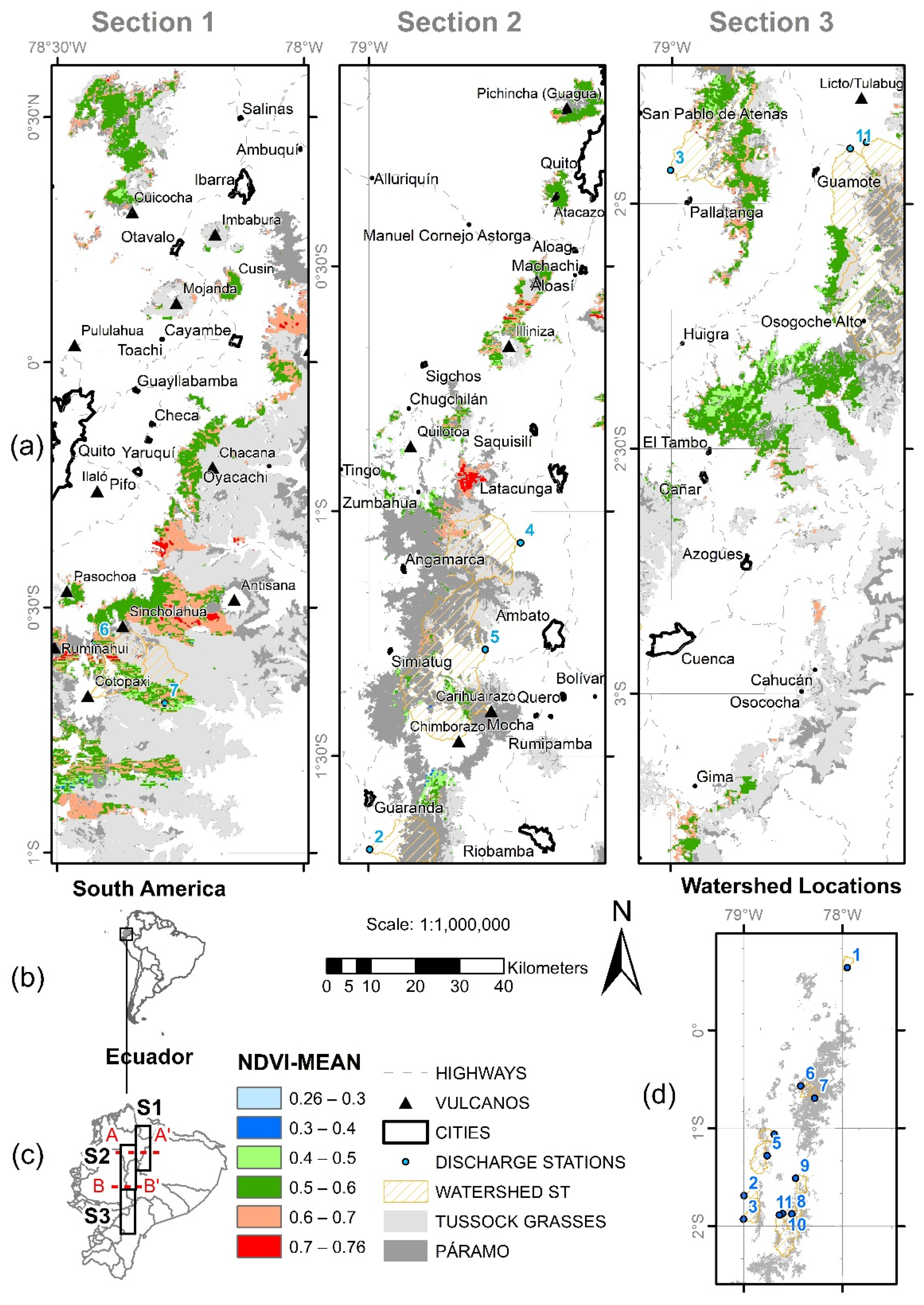
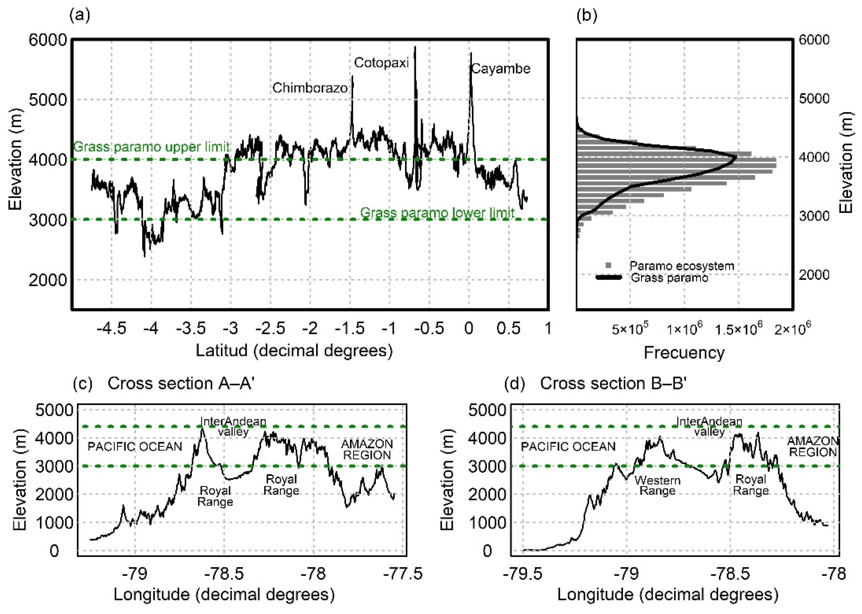
2.1. Study Area

| Coast | Highlands | Amazon | |
|---|---|---|---|
| Average annual air temperature (°C) | 25.5 | 12.7 | 21.8 |
| Average annual rainfall (mm/year) | 892.9 | 798.9 | 3449.4 |
| Rainy season | January to April | Mar to April and October to November | Almost the whole year 1 |
| Dry season | June to December | May to September and December to January | August to January |
2.2. Time Series of Vegetation Indices, Climate Information and Global Teleconnection Indices
2.2.1. NDVI Dataset
2.2.2. Satellite Climate Information and Water Availability
2.2.3. Global Teleconnection Indices
2.3. Methods
2.3.1. Spatio-Temporal Analysis of NDVI
2.3.2. NDVI Analysis—Climatic Variables and Water Availability
2.3.3. NDVI Analysis—Global Climate Indices
3. Results
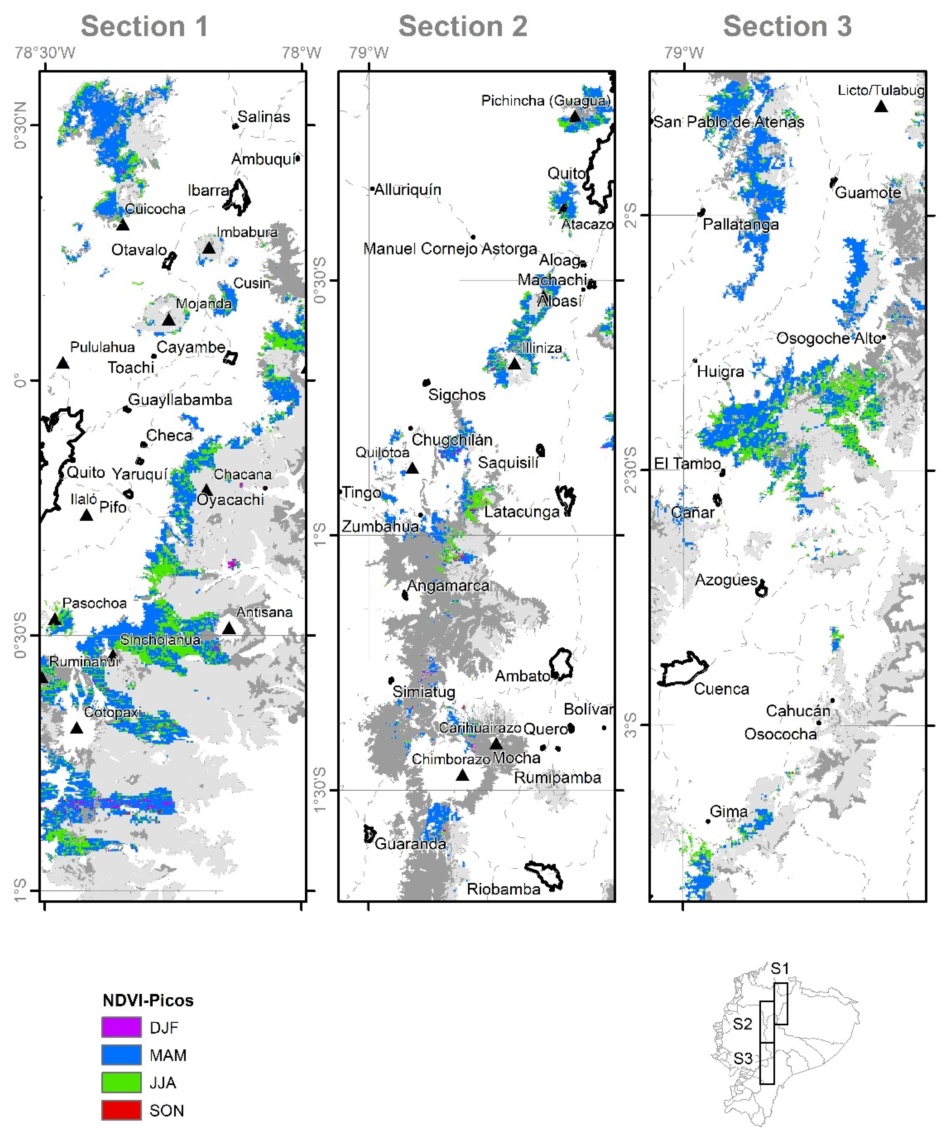
3.1. Spatio-Temporal Analysis of NDVI
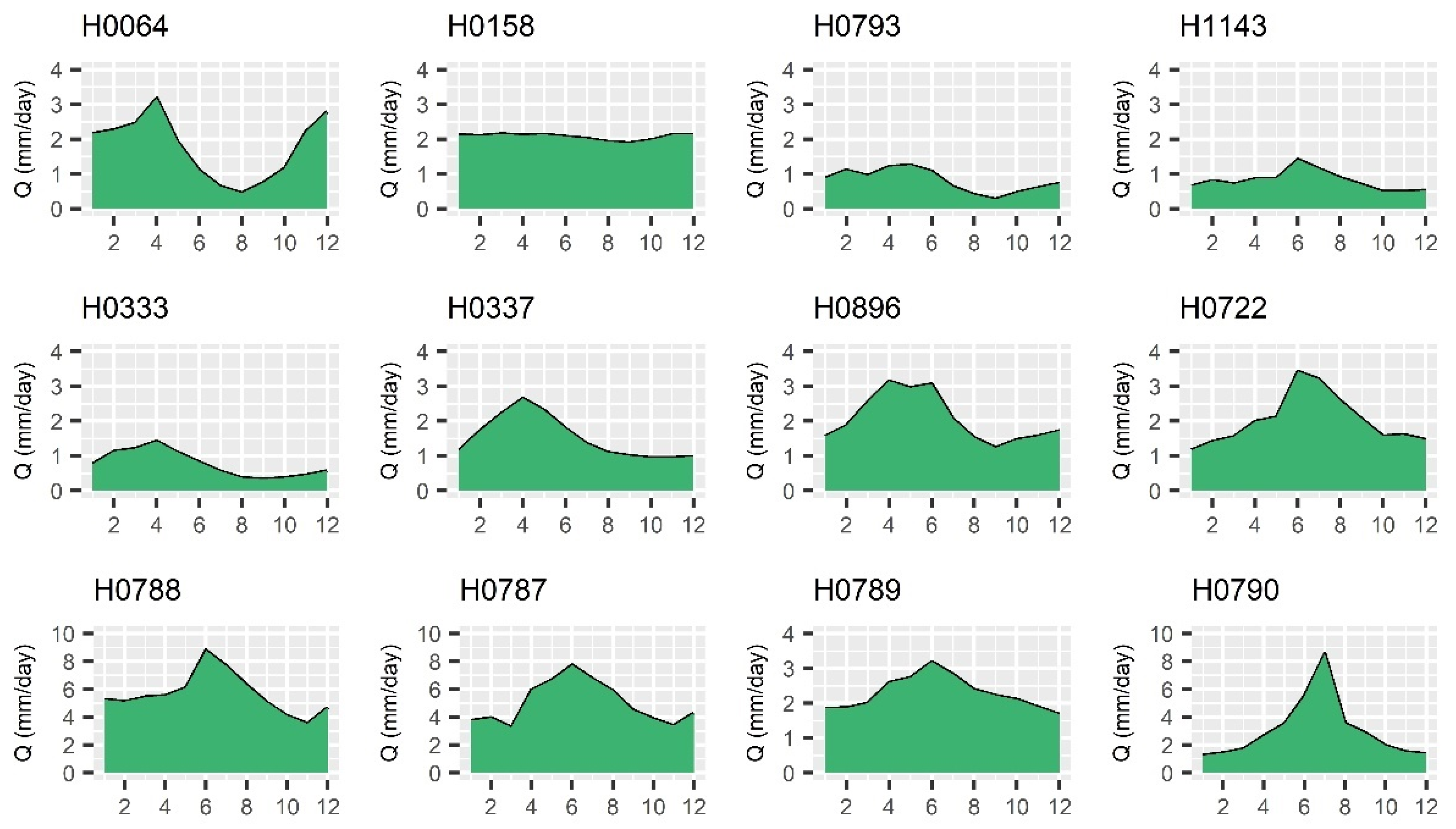
3.2. NDVI Analysis—Climatic Variables and Water Availability
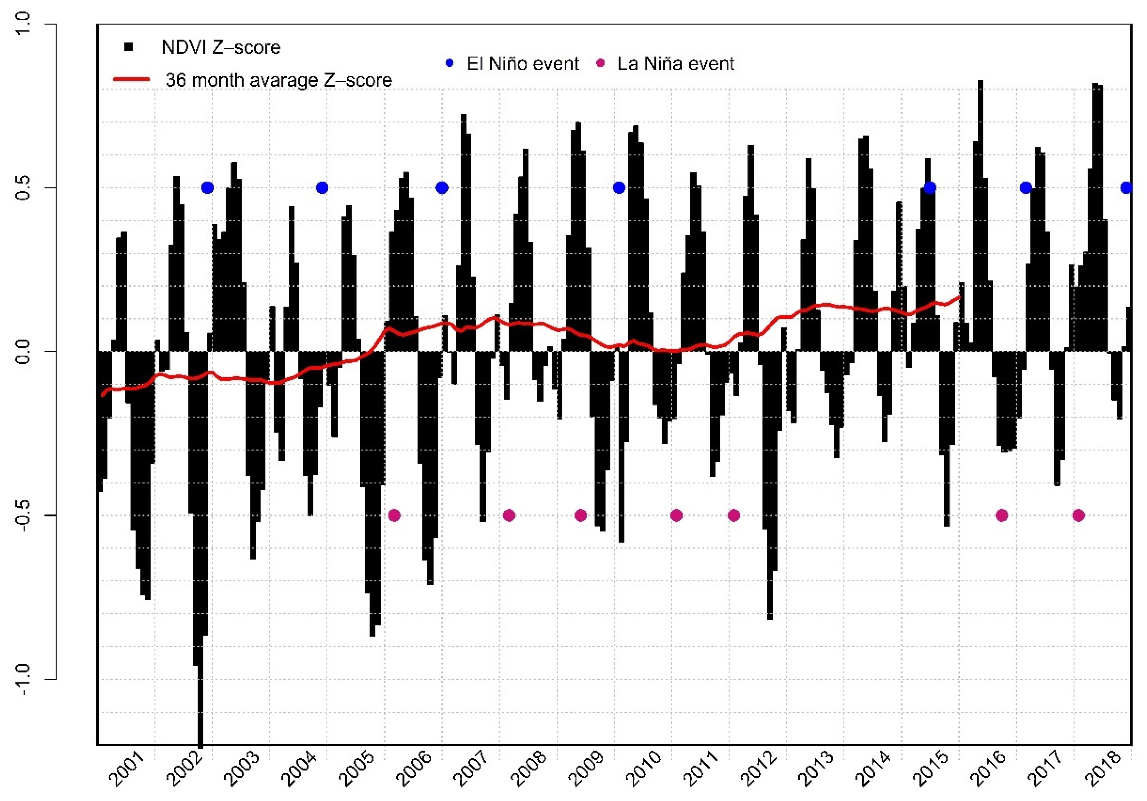
3.3. NDVI Analysis—Global Climate Indices
4. Discussion
4.1. Spatio-Temporal Analysis of NDVI
4.2. NDVI Analysis—Climatic Variables
4.3. NDVI Analysis—Global Climate Indices
5. Conclusions
Author Contributions
Funding
Institutional Review Board Statement
Informed Consent Statement
Data Availability Statement
Conflicts of Interest
References
- Lauer, W. Ecoclimatological Conditions of the Paramo Belt in the Tropical High Mountains. Int. Mt. Soc. Stable 1981, 1, 209–221. [Google Scholar] [CrossRef]
- Garreaud, R.D.; Vuille, M.; Compagnucci, R.; Marengo, J. Present-Day South American Climate. Palaeogeogr. Palaeoclim. Palaeoecol. 2009, 281, 180–195. [Google Scholar] [CrossRef]
- Harden, C.P. Human Impacts on Headwater Fluvial Systems in the Northern and Central Andes. Geomorphology 2006, 79, 249–263. [Google Scholar] [CrossRef]
- Vuille, M.; Bradley, R.S.; Keimig, F. Climate Variability in the Andes of Ecuador and Its Relation to Tropical Pacific and Atlantic Sea Surface Temperature Anomalies. J. Clim. 2000, 13, 2520–2535. [Google Scholar] [CrossRef]
- Jørgensen, P.M.; León-Yánez, S. Catalogue of the Vascular Plants of Ecuador; Missouri Botanical Garden Press: St. Louis, MO, USA, 1999; Volume 75. [Google Scholar]
- Pourrut, P.; Pouyaud, B. El Agua En El Ecuador: Clima, Precipitaciones, Escorrentía; Corporación Editora Nacional: Quito, Ecuador, 1995. [Google Scholar]
- Junquas, C.; Heredia, M.B.; Condom, T.; Ruiz-Hernández, J.C.; Campozano, L.; Dudhia, J.; Espinoza, J.C.; Menegoz, M.; Rabatel, A.; Sicart, J.E. Regional Climate Modeling of the Diurnal Cycle of Precipitation and Associated Atmospheric Circulation Patterns over an Andean Glacier Region (Antisana, Ecuador). Clim. Dyn. 2022, 58, 3075–3104. [Google Scholar] [CrossRef]
- Buytaert, W.; de Bievre, B. Water for Cities: The Impact of Climate Change and Demographic Growth in the Tropical Andes. Water Resour. Res. 2012, 48. [Google Scholar] [CrossRef]
- Viviroli, D.; Archer, D.R.; Buytaert, W.; Fowler, H.J.; Greenwood, G.B.; Hamlet, A.F.; Huang, Y.; Koboltschnig, G.; Litaor, M.I.; López-Moreno, J.I.; et al. Climate Change and Mountain Water Resources: Overview and Recommendations for Research, Management and Policy. Hydrol. Earth Syst. Sci. 2011, 15, 471–504. [Google Scholar] [CrossRef]
- Hamel, P.; Riveros-Iregui, D.; Ballari, D.; Browning, T.; Célleri, R.; Chandler, D.; Chun, K.P.; Destouni, G.; Jacobs, S.; Jasechko, S.; et al. Watershed Services in the Humid Tropics: Opportunities from Recent Advances in Ecohydrology. Ecohydrology 2018, 11, e1921. [Google Scholar] [CrossRef]
- Ponette-González, A.G.; Marín-Spiotta, E.; Brauman, K.A.; Farley, K.A.; Weathers, K.C.; Young, K.R. Hydrologic Connectivity in the High-Elevation Tropics: Heterogeneous Responses to Land Change. Bioscience 2014, 64, 92–104. [Google Scholar]
- Appenzeller, T. Fire on the Mountain. Science 2019, 365, 1094–1097. [Google Scholar] [CrossRef]
- Huete, A.; Didan, K.; Miura, T.; Rodriguez, E.P.; Gao, X.; Ferreira, L.G. Overview of the Radiometric and Biophysical Performance of the MODIS Vegetation Indices. Remote Sens. Environ. 2002, 83, 195–213. [Google Scholar] [CrossRef]
- Justice, C.; Townshend, J.; Holben, A.; Tucker, C. Analysis of the Phenology of Global Vegetation Using Meteorological Satellite Data. Int. J. Remote Sens. 1985, 6, 1271–1318. [Google Scholar] [CrossRef]
- Tucker, C.J.; Sellers, P.J. Satellite Remote Sensing of Primary Production. Int. J. Remote Sens. 1986, 7, 1395–1416. [Google Scholar] [CrossRef]
- Delire, C.; de Noblet-Ducoudré, N.; Sima, A.; Gouirand, I. Vegetation Dynamics Enhancing Long-Term Climate Variability Confirmed by Two Models. J. Clim. 2011, 24, 2238–2257. [Google Scholar] [CrossRef]
- Li, Z.; Huffman, T.; McConkey, B.; Townley-Smith, L. Monitoring and Modeling Spatial and Temporal Patterns of Grassland Dynamics Using Time-Series MODIS NDVI with Climate and Stocking Data. Remote Sens. Environ. 2013, 138, 232–244. [Google Scholar] [CrossRef]
- Myneni, R.B.; Hall, F.G.; Sellers, P.J.; Marshak, A.L. Interpretation of Spectral Vegetation Indexes. IEEE Trans. Geosci. Remote Sens. 1995, 33, 481–486. [Google Scholar] [CrossRef]
- Paruelo, J.M.; Epstein, H.E.; Lauenroth, W.K.; Burke, I.C. ANPP Estimates from NDVI for the Central Grassland Region of the United States. Ecology 1997, 78, 953–958. [Google Scholar] [CrossRef]
- Gamon, J.A.; Field, C.B.; Goulden, M.L.; Griffin, K.L.; Hartley, A.E.; Joel, G.; Penuelas, J.; Valentini, R. Relationships between NDVI, Canopy Structure, and Photosynthesis in Three Californian Vegetation Types. Ecol. Appl. 1995, 5, 28–41. [Google Scholar] [CrossRef]
- Arboit, M.E.; Maglione, D.S. Categorización de Las Manzanas Urbanas Para La Integración de La Silvicultura Urbana En La Planificación de Las Ciudades. Caso de Estudio: Área Metropolitana de Mendoza, Argentina. III Congr. Int. Isuf-H. Ciudad. Compact. Vs. Ciudad. Difusa 2020, 297–305. [Google Scholar] [CrossRef]
- Burgheimer, J.; Wilske, B.; Maseyk, K.; Karnieli, A.; Zaady, E.; Yakir, D.; Kesselmeier, J. Relationships between Normalized Difference Vegetation Index (NDVI) and Carbon Fluxes of Biologic Soil Crusts Assessed by Ground Measurements. J. Arid. Environ. 2006, 64, 651–669. [Google Scholar] [CrossRef]
- Kunkel, M.L.; Flores, A.N.; Smith, T.J.; McNamara, J.P.; Benner, S.G. A Simplified Approach for Estimating Soil Carbon and Nitrogen Stocks in Semi-Arid Complex Terrain. Geoderma 2011, 165, 1–11. [Google Scholar] [CrossRef]
- Gu, Y.; Brown, J.F.; Verdin, J.P.; Wardlow, B. A Five-Year Analysis of MODIS NDVI and NDWI for Grassland Drought Assessment over the Central Great Plains of the United States. Geophys. Res. Lett. 2007, 34. [Google Scholar] [CrossRef]
- Dayeh, M.A.; Desai, M.I.; Dwyer, J.R.; Rassoul, H.K.; Mason, G.M.; Mazur, J.E. Composition and Spectral Properties of the 1 Au Quiet-Time Suprathermal Ion Population during Solar Cycle 23. Astrophys. J. 2009, 693, 1588–1600. [Google Scholar] [CrossRef]
- Mewaldt, R.A.; Looper, M.D.; Cohen, C.M.S.; Haggerty, D.K.; Labrador, A.W.; Leske, R.A.; Mason, G.M.; Mazur, J.E.; von Rosenvinge, T.T. Energy Spectra, Composition, and Other Properties of Ground-Level Events during Solar Cycle 23. Space Sci. Rev. 2012, 171, 97–120. [Google Scholar] [CrossRef]
- Schweiger, A.K.; Cavender-Bares, J.; Townsend, P.A.; Hobbie, S.E.; Madritch, M.D.; Wang, R.; Tilman, D.; Gamon, J.A. Plant Spectral Diversity Integrates Functional and Phylogenetic Components of Biodiversity and Predicts Ecosystem Function. Nat. Ecol. Evolume 2018, 2, 976–982. [Google Scholar] [CrossRef] [PubMed]
- Wang, K.; Franklin, S.E.; Guo, X.; Cattet, M. Remote Sensing of Ecology, Biodiversity and Conservation: A Review from the Perspective of Remote Sensing Specialists. Sensors 2010, 10, 9647–9667. [Google Scholar] [CrossRef] [PubMed]
- Wang, R.; Gamon, J.A.; Cavender-Bares, J.; Townsend, P.A.; Zygielbaum, A.I. The Spatial Sensitivity of the Spectral Diversity-Biodiversity Relationship: An Experimental Test in a Prairie Grassland. Ecol. Appl. 2018, 28, 541–556. [Google Scholar] [CrossRef]
- Eklundh, L.; Jönsson, P. TIMESAT for Processing Time-Series Data from Satellite Sensors for Land Surface Monitoring. In Multitemporal Remote Sensing; Ban, Y., Ed.; Springer: Cham, Switzerland, 2016; Volume 20. [Google Scholar] [CrossRef]
- Moreira, A.; Bremm, C.; Fontana, D.C.; Kuplich, T.M. Seasonal Dynamics of Vegetation Indices as a Criterion for Grouping Grassland Typologies. Sci. Agricola 2019, 76, 24–32. [Google Scholar] [CrossRef]
- van Leeuwen, W.J.D.; Hartfield, K.; Miranda, M.; Meza, F.J. Trends and ENSO/AAO Driven Variability in NDVI Derived Productivity and Phenology alongside the Andes Mountains. Remote Sens. 2013, 5, 1177–1203. [Google Scholar] [CrossRef]
- Walther, G.R.; Post, E.; Convey, P.; Menzel, A.; Parmesan, C.; Beebee, T.J.C.; Fromentin, J.M.; Hoegh-Guldberg, O.; Bairlein, F. Ecological Responses to Recent Climate Change. Nature 2002, 416, 389–395. [Google Scholar] [CrossRef]
- Li, H.; Liu, L.; Liu, X.; Li, X.; Xu, Z. Greening Implication Inferred from Vegetation Dynamics Interacted with Climate Change and Human Activities over the Southeast Qinghai-Tibet Plateau. Remote Sens. 2019, 11, 2421. [Google Scholar] [CrossRef]
- IPCC. Climate Change 2007: Impacts, Adaptation and Vulnerability: Contribution of Working Group II to the Fourth Assessment Report of the Intergovernmental Panel; Cambridge University Press: Cambridge, UK, 2007. [Google Scholar]
- Roerink, G.J.; Menenti, M.; Soepboer, W.; Su, Z. Assessment of Climate Impact on Vegetation Dynamics by Using Remote Sensing. Phys. Chem. Earth 2003, 28, 103–109. [Google Scholar] [CrossRef]
- Cleland, E.E.; Chiariello, N.R.; Loarie, S.R.; Mooney, H.A.; Field, C.B. Diverse Responses of Phenology to Global Changes in a Grassland Ecosystem. Proc. Natl. Acad. Sci. USA 2006, 103, 13740–13744. [Google Scholar] [CrossRef] [PubMed]
- Myneni, R.B.; Keeling, C.D.; Tucker, C.J.; Asrar, G.; Nemani, R.R. Increased Plant Growth in the Northern High Latitudes from 1981 to 1991. Nature 1997, 386, 698–702. [Google Scholar] [CrossRef]
- Schwartz, M.D.; Ahas, R.; Aasa, A. Onset of Spring Starting Earlier across the Northern Hemisphere. Glob. Chang. Biol. 2006, 12, 343–351. [Google Scholar] [CrossRef]
- Justice, C.; Vermote, E.; Townshend, J.; Defries, R.; Roy, D.; Hall, D.; Salomonson, V.; Privette, J.; Riggs, G.; Strahler, A.; et al. The Moderate Resolution Imaging Spectroradiometer (MODIS): Land Remote Sensing for Global Change Research. IEEE Trans. Geosci. Remote Sens. 1998, 36, 1228–1249. [Google Scholar] [CrossRef]
- Zhang, X.; Friedl, M.A.; Schaaf, C.B. Global Vegetation Phenology from Moderate Resolution Imaging Spectroradiometer (MODIS): Evaluation of Global Patterns and Comparison with in Situ Measurements. J. Geophys. Res. Biogeosci. 2006, 111. [Google Scholar] [CrossRef]
- Li, Z.; Li, X.; Wei, D.; Xu, X.; Wang, H. An Assessment of Correlation on MODIS-NDVI and EVI with Natural Vegetation Coverage in Northern Hebei Province, China. Procedia Environ. Sci. 2010, 2, 964–969. [Google Scholar] [CrossRef]
- Viña, A.; Henebry, G.M. Spatio-Temporal Change Analysis to Identify Anomalous Variation in the Vegetated Land Surface: ENSO Effects in Tropical South America. Geophys. Res. Lett. 2005, 32. [Google Scholar] [CrossRef]
- Poveda, G.; Álvarez, D.M.; Rueda, Ó.A. Hydro-Climatic Variability over the Andes of Colombia Associated with ENSO: A Review of Climatic Processes and Their Impact on One of the Earth’s Most Important Biodiversity Hotspots. Clim. Dyn. 2010, 36, 2233–2249. [Google Scholar] [CrossRef]
- Silvia, L.; Alexander, T.; Anna, K.; Polina, K. Assessment of carbon dynamics in Ecuadorian forests through the Mathematical Spatial Model of Global Carbon Cycle and the Normalized Differential Vegetation Index (NDVI). E3S Web Conf. 2019, 96, 02002. [Google Scholar] [CrossRef]
- Chamorro Sevilla, H.E.; Erazo, A. Estudio Multiespectral Del Cultivo de Tuna Para Determinar Los Índices NDVI, CWSI y SAVI, a Partir de Imágenes SENTINEL 2A, En El Cantón Guano, Provincia de Chimborazo, Ecuador. Enfoque UTE 2019, 10, 55–66. [Google Scholar] [CrossRef]
- Myers, N.; Mittermeler, R.A.; Mittermeler, C.G.; da Fonseca, G.A.B.; Kent, J. Biodiversity Hotspots for Conservation Priorities. Nature 2000, 403, 853–858. [Google Scholar] [CrossRef] [PubMed]
- Mena, P.; Hofstede, R. The Ecuadorian Páramos. Botánica Económica de Los Andes Centrales; Universidad Mayor de San Andrés: La Paz, Bolivia, 2006. [Google Scholar]
- Madriñán, S.; Cortés, A.J.; Richardson, J.E. Páramo Is the World’s Fastest Evolving and Coolest Biodiversity Hotspot. Front. Genet. 2013, 4, 192. [Google Scholar] [CrossRef]
- Hofstede, R. Los Servicios Del Ecosistema Páramo: Una Visión Desde La Evaluación de Ecosistemas Del Milenio; EcoCiencia: Quito, Ecuador, 2008. [Google Scholar]
- Morales, J.A.; Estévez, J.V. El Páramo: ¿Ecosistema En Vía De Extinción? Rev. Luna Azul 2006, 22, 39–51. [Google Scholar]
- Buytaert, W.; Wyseure, G.; de Bièvre, B.; Deckers, J. The Effect of Land-Use Changes on the Hydrological Behaviour of Histic Andosols in South Ecuador. Hydrol. Process. 2005, 19, 3985–3997. [Google Scholar] [CrossRef]
- Grau, R.; Aide, M. Globalization and Land-Use Transitions in Latin America. Ecol. Soc. 2008, 13. [Google Scholar] [CrossRef]
- Wang, J.; Rich, P.M.; Price, K.P. Temporal Responses of NDVI to Precipitation and Temperature in the Central Great Plains, USA. Int. J. Remote Sens. 2003, 24, 2345–2364. [Google Scholar] [CrossRef]
- Zhang, X.; Friedl, M.A.; Schaaf, C.B.; Strahler, A.H.; Hodges, J.C.F.; Gao, F.; Reed, B.C.; Huete, A. Monitoring Vegetation Phenology Using MODIS. Remote Sens. Environ. 2003, 84, 471–475. [Google Scholar] [CrossRef]
- Duan, S.B.; Li, Z.L.; Li, H.; Göttsche, F.M.; Wu, H.; Zhao, W.; Leng, P.; Zhang, X.; Coll, C. Validation of Collection 6 MODIS Land Surface Temperature Product Using in Situ Measurements. Remote Sens. Environ. 2019, 225, 16–29. [Google Scholar] [CrossRef]
- Krakauer, N.Y.; Pradhanang, S.M.; Lakhankar, T.; Jha, A.K. Evaluating Satellite Products for Precipitation Estimation in Mountain Regions: A Case Study for Nepal. Remote Sens. 2013, 5, 4107–4123. [Google Scholar] [CrossRef]
- Kalisa, W.; Igbawua, T.; Henchiri, M.; Ali, S.; Zhang, S.; Bai, Y.; Zhang, J. Assessment of Climate Impact on Vegetation Dynamics over East Africa from 1982 to 2015. Sci. Rep. 2019, 9, 16865. [Google Scholar] [CrossRef] [PubMed]
- Kaser, G. Glacier-Climate Interaction at Low Latitudes. J. Glaciol. 2001, 47, 195–204. [Google Scholar] [CrossRef]
- Thompson, L.G. Ice Core Evidence for Climate Change in the Tropics: Implications for Our Future. Quat. Sci. Rev. 2000, 19, 19–35. [Google Scholar] [CrossRef]
- Jomelli, V.; Cooley, D.; Naveau, P.; Rabatel, A. The Little Ice Age in the Tropical Andes. In Proceedings of the American Geophysical Union: Fall 2003 Conference, San Francisco, USA, 1 December 2003. PP51A-07. [Google Scholar]
- Cerón, C.; Palacios, W.; Valencia, R.; Sierra, R. Las Formaciones Naturales de La Amazonía Del Ecuador. In Propuesta Preliminar de un Sistema de Clasificación de Vegetación para el Ecuador Continental; Sierra, R., Ed.; Editorial Rimana: Quito, Ecuador, 1999; pp. 111–119. [Google Scholar]
- INEC. Encuesta de Superficie y Producción Agropecuaria Continua; Independent National Electoral Commission: Ilocos Norte, Philippines, 2018. [Google Scholar]
- Vallejo, M.C.; Sacher, W. Encyclopedia of Mineral and Energy Policy; Tiess, G., Majumder, T., Cameron, P., Eds.; Springer: Berlin/Heidelberg, Germany, 2017. [Google Scholar] [CrossRef]
- Standmuller, T. Cloud Forests in the Humid Tropics: A Bibliographic Review; United Nations University Press: Tokyo, Japan, 1986. [Google Scholar]
- Young, B.E.; Young, K.R.; Josse, C. Vulnerability of Tropical Andean Ecosystems to Climate Change. Clim. Chang. Biodivers. Trop. Andes 2011, 1, 12. [Google Scholar]
- Ramsay, P.M. The Paramo Vegetation of Ecuador: The Community Ecology, Dynamics and Productivity of Tropical Grasslands in the Andes; Bangor University: Bangor, UK, 1992. [Google Scholar]
- Buytaert, W.; Iñiguez, V.; Celleri, R.; de Bièvre, B.; Wyseure, G.; Deckers, J. Analysis of the Water Balance of Small Páramo Catchments in South Ecuador. Environ. Role Wetl. Headwaters 2006, 63, 271–281. [Google Scholar] [CrossRef]
- Farley, J.; Aquino, A.; Daniels, A.; Moulaert, A.; Lee, D.; Krause, A. Global Mechanisms for Sustaining and Enhancing PES Schemes. Ecol. Econ. 2010, 69, 2075–2084. [Google Scholar] [CrossRef]
- Harling, G. The Vegetation Types of Ecuador: A Brief Survey. In Tropical Botany; Larsen, K., Holm-Nielsen, L.B., Eds.; Academic Press: London, UK, 1979; pp. 165–174. [Google Scholar]
- Pourrut, P.; Acosta, J.; Winckell, A.; Rodriguez, J. Los Climas Del Ecuador; Centro Ecuatoriano de Investigación Geográfica: Quito, Ecuador, 1983. [Google Scholar]
- Alcaraz-Segura, D.; Baldi, G.; Durante, P.; Garbulsky, M.F. Análisis de La Dinámica Temporal Del NDVI En Áreas Protegidas: Tres Casos de Estudio a Distintas Escalas Espaciales, Temporales y de Gestión. Ecosistemas 2008, 17, 108–117. [Google Scholar]
- Tiedemann, J.; Zerda, H.; Grilli, M.; Ravelo, A. Distribución Espacial de Anomalías Del NDVI Derivado Del Sensor VEGETATION SPOT 4/5 y Su Relación Con Las Coberturas Vegetales, Usos de La Tierra y Características Geomorfológicas En La Provincia de Santiago Del Estero, Argentina. Rev. Ambiência 2010, 6, 379–391. [Google Scholar] [CrossRef][Green Version]
- Veettil, B.K.; Pereira, S.F.R.; Wang, S.; Valente, P.T.; Grondona, A.E.B.; Rondón, A.C.B.; Rekowsky, I.C.; de Souza, S.F.; Bianchini, N.; Bremer, U.F.; et al. Un Análisis Comparativo Del Comportamiento Diferencial de Los Glaciares En Los Andes Tropicales Usando Teledetección. Investig. Geográficas 2016, 3–36. [Google Scholar] [CrossRef]
- Zoffoli, M.L.; Madanes, N.; Kandus, P. Contribución de Series Temporales de NDVI NOAA/AVHRR al Análisis Funcional En Humedales. In Proceedings of the Anais XIII Simposio Brasileiro de Sensoramiento Remoto, Florianópolis, Brasil, 21–26 Apri1 2007. [Google Scholar]
- Manan, P.; Shital, S.; Kalubarme, M.H. Impact of Climate Change and Drought Analysis on Agriculture In Sabarkantha Districtusing Geoinformatics Technology. Glob. J. Eng. Sci. Res. 2019, 6, 133–144. [Google Scholar]
- Tucker, C.J.; Pinzon, J.E.; Brown, M.E.; Slayback, D.A.; Pak, E.W.; Mahoney, R.; Vermote, E.F.; el Saleous, N. An Extended AVHRR 8-Km NDVI Dataset Compatible with MODIS and SPOT Vegetation NDVI Data. Int. J. Remote Sens. 2005, 26, 4485–4498. [Google Scholar] [CrossRef]
- MAE SIstema de Clasificación de Los Ecosistemas Del Ecuador Continental; Ministerio del Ambiente: Magdalena del Mar, Peru, 2013.
- Jiang, X.; Was, L.; Du, Q.; Hu, B.X. Estimation of NDVI Images Using Geostatistical Methods. Earth Sci. Front. 2008, 15, 71–80. [Google Scholar] [CrossRef]
- Schafer, R.W. What Is a Savitzky-Golay Filter? IEEE Signal. Process. Mag. 2011, 28, 111–117. [Google Scholar] [CrossRef]
- Funk, C.; Peterson, P.; Landsfeld, M.; Pedreros, D.; Verdin, J.; Shukla, S.; Husak, G.; Rowland, J.; Harrison, L.; Hoell, A.; et al. The Climate Hazards Infrared Precipitation with Stations—A New Environmental Record for Monitoring Extremes. Sci. Data 2015, 2, 150066. [Google Scholar] [CrossRef] [PubMed]
- Wan, Z. A Generalized Split-Window Algorithm for Retrieving Land-Surface Temperature from Space. IEEE Trans. Geosci. Remote Sens. 1996, 34, 892–905. [Google Scholar] [CrossRef]
- Stenseth, N.C.; Ottersen, G.; Hurrell, J.W.; Mysterud, A.; Lima, M.; Chan, K.S.; Yoccoz, N.G.; Ådlandsvik, B. Studying Climate Effects on Ecology through the Use of Climate Indices: The North Atlantic Oscillation, El Niño Southern Oscillation and Beyond. Proc. R. Soc. B Biol. Sci. 2003, 270, 2087–2096. [Google Scholar] [CrossRef]
- Hill, M.J.; Donald, G.E. Estimating Spatio-Temporal Patterns of Agricultural Productivity in Fragmented Landscapes Using Avhrr NDVI Time Series. Remote Sens. Environ. 2003, 84, 367–384. [Google Scholar] [CrossRef]
- de Beurs, K.; Wright, C.; Henebry, G. Dual Scale Trend Analysis for Evaluating Climatic and Anthropogenic Effects on the Vegetated Land Surface in Russia and Kazakhstan. Environ. Res. Lett. 2009, 4, 040512. [Google Scholar] [CrossRef]
- de Beurs, K.; Henebry, G. Spatio-Temporal Statistical Methods for Modelling Land Surface Phenology. In Phenological Research: Methods for Environmental and Climate Change Analysis; Springer: Dordrecht, The Netherlands, 2010; pp. 177–208. ISBN 9789048133352. [Google Scholar]
- Sen, P.K. Estimates of the Regression Coefficient Based on Kendall’s Tau. J. Am. Stat. Assoc. 1968, 63, 1379–1389. [Google Scholar] [CrossRef]
- Benesty, J.; Chen, J.; Huang, Y.; Cohen, I. Noise Reduction in Speech Processing; Springer: Berlin/Heidelberg, Germany, 2009; Volume 2. [Google Scholar]
- Haigh, J.; Conover, W.J. Practical Nonparametric Statistics. J. R. Stat. Soc. Ser. A 1981, 144, 370. [Google Scholar] [CrossRef]
- Yan, Z.; Wang, S.; Ma, D.; Liu, B.; Lin, H.; Li, S. Meteorological Factors Affecting Pan Evaporation in the Haihe River Basin, China. Water 2019, 11, 317. [Google Scholar] [CrossRef]
- Minaya, V.; Corzo, G.; Romero-Saltos, H.; van der Kwast, J.; Lantinga, E.; Galárraga-Sánchez, R.; Mynett, A. Altitudinal Analysis of Carbon Stocks in the Antisana Páramo, Ecuadorian Andes. J. Plant Ecol. 2016, 9, 553–563. [Google Scholar] [CrossRef]
- Ramsay, P.M.; Oxley, E.R.B. An Assessment of Aboveground Net Primary Productivity in Andean Grasslands of Central Ecuador. Source Mt. Res. Dev. 2001, 21, 161–167. [Google Scholar] [CrossRef]
- Ilbay-Yupa, M.; Lavado-Casimiro, W.; Rau, P.; Zubieta, R.; Castillón, F. Updating Regionalization of Precipitation in Ecuador. Theor. Appl. Clim. 2021, 143, 1513–1528. [Google Scholar] [CrossRef]
- Domínguez-Castro, F.; García-Herrera, R.; Vicente-Serrano, S.M. Wet and Dry Extremes in Quito (Ecuador) since the 17th Century. Int. J. Climatol. 2018, 38, 2006–2014. [Google Scholar] [CrossRef]
- Emck, P. A Climatology of South Ecuador—With Special Focus on the Major Andean Ridge as Atlantic-Pacific Climate Divide; University of Erlangen–Nuremberg: Erlangen, Germany, 2007; Volume 1. [Google Scholar]
- Rollenbeck, R.; Bendix, J. Rainfall Distribution in the Andes of Southern Ecuador Derived from Blending Weather Radar Data and Meteorological Field Observations. Atmos. Res. 2011, 99, 277–289. [Google Scholar] [CrossRef]
- Estrella, E.H.; Stoeth, A.; Krakauer, N.Y.; Devineni, N. Quantifying Vegetation Response to Environmental Changes on the Galapagos Islands, Ecuador Using the Normalized Difference Vegetation Index (NDVI). Environ. Res. Commun. 2021, 3, 065003. [Google Scholar] [CrossRef]
- Haverd, V.; Smith, B.; Canadell, J.G.; Cuntz, M.; Mikaloff-Fletcher, S.; Farquhar, G.; Woodgate, W.; Briggs, P.R.; Trudinger, C.M. Higher than Expected CO2 Fertilization Inferred from Leaf to Global Observations. Glob. Chang. Biol. 2020, 26, 2390–2402. [Google Scholar] [CrossRef]
- Vega-Jácome, F. Respuesta de La Vegetación a Diferentes Escalas Temporales de Sequía En Los Andes Peruanos. Serv. Nac. De Meteorol. E Hidrol. Del Perú. 2019. Available online: https://repositorio.senamhi.gob.pe/handle/20.500.12542/294 (accessed on 28 June 2022).
- Mazzarino, M.; Finn, J.T. An NDVI Analysis of Vegetation Trends in an Andean Watershed. Wetl. Ecol. Manag. 2016, 24, 623–640. [Google Scholar] [CrossRef]
- Chen, M.; Parton, W.J.; Hartman, M.D.; del Grosso, S.J.; Smith, W.K.; Knapp, A.K.; Lutz, S.; Derner, J.D.; Tucker, C.J.; Ojima, D.S.; et al. Assessing Precipitation, Evapotranspiration, and NDVI as Controls of U.S. Great Plains Plant Production. Ecosphere 2019, 10, e02889. [Google Scholar] [CrossRef]
- Álvarez-Dávila, E.A.; Cayuela, L.; González-Caro, S.; Aldana, A.M.; Stevenson, P.R.; Phillips, O.; Lvaro Cogollo, A.; Peñuela, M.C.; von Hildebrand, P.; Jimpenez, E.; et al. Forest Biomass Density across Large Climate Gradients in Northern South America Is Related to Water Availability but Not with Temperature. PLoS ONE 2017, 12, e0171072. [Google Scholar] [CrossRef] [PubMed]
- Girardin, C.A.J.; Espejob, J.E.S.; Doughty, C.E.; Huasco, W.H.; Metcalfe, D.B.; Durand-Baca, L.; Marthews, T.R.; Aragao, L.E.O.C.; Farfán-Rios, W.; García-Cabrera, K.; et al. Productivity and Carbon Allocation in a Tropical Montane Cloud Forest in the Peruvian Andes. Plant Ecol. Divers. 2014, 7, 107–123. [Google Scholar] [CrossRef]
- Spracklen, D.V.; Righelato, R. Tropical Montane Forests Are a Larger than Expected Global Carbon Store. Biogeosciences 2014, 11, 2741–2754. [Google Scholar] [CrossRef]
- Laraque, A.; Ronchail, J.; Cochonneau, G.; Pombosa, R.; Guyot, J.L. Heterogeneous Distribution of Rainfall and Discharge Regimes in the Ecuadorian Amazon Basin. J. Hydrometeorol. 2007, 8, 1364–1381. [Google Scholar] [CrossRef]
- Vaca-Jiménez, S.; Gerbens-Leenes, P.W.; Nonhebel, S. Water-Electricity Nexus in Ecuador: The Dynamics of the Electricity’s Blue Water Footprint. Sci. Total Environ. 2019, 696, 133959. [Google Scholar] [CrossRef]
- Crespo, P.J.; Feyen, J.; Buytaert, W.; Bücker, A.; Breuer, L.; Frede, H.G.; Ramírez, M. Identifying Controls of the Rainfall–Runoff Response of Small Catchments in the Tropical Andes (Ecuador). J. Hydrol. 2011, 407, 164–174. [Google Scholar] [CrossRef]
- Reich, P.B.; Luo, Y.; Bradford, J.B.; Poorter, H.; Perry, C.H.; Oleksyn, J. Temperature Drives Global Patterns in Forest Biomass Distribution in Leaves, Stems, and Roots. Proc. Natl. Acad. Sci. USA 2014, 111, 13721–13726. [Google Scholar] [CrossRef]
- Rapp, J.M.; Silman, M.R.; Clark, J.S.; Girardin, C.A.J.; Galiano, D.; Tito, R.; Doak, D.F. Intra- and Interspecific Tree Growth across a Long Altitudinal Gradient in the Peruvian Andes. Ecology 2012, 93, 2061–2072. [Google Scholar] [CrossRef]
- Bendix, J. Precipitation Dynamics in Ecuador and Northern Peru during the 1991/92 El Nino: A Remote Sensing Perspective. Int. J. Remote Sens. 2000, 21, 533–548. [Google Scholar] [CrossRef]
- Bendix, J.; Trachte, K.; Palacios, E.; Rollenbeck, R.; Göttlicher, D.; Nauss, T.; Bendix, A. El Niño Meets La Niña-Anomalous Rainfall Patterns in the “Traditional” El Niño Region of Southern Ecuador. Erdkunde 2011, 65, 151–167. [Google Scholar] [CrossRef]
- Cárdenas, G. Teleconexión El Niño-Oscilación Del Sur/Oscilación Del Atlántico Norte y Su Relación Con La Precipitación En Colombia; Universidad de Bogotá Jorge Tadeo Lozano: Bogotá, Colombia, 2022. [Google Scholar]
- Francou, B.; Vuille, M.; Favier, V.; Cáceres, B. New Evidence for an ENSO Impact on Low-Latitude Glaciers: Antizana 15, Andes of Ecuador, 0°28′S. J. Geophys. Res. Atmos. 2004, 109, D18106. [Google Scholar] [CrossRef]
- Lavad-Casimiro, W.S.; Labat, D.; Ronchail, J.; Espinoza, J.C.; Guyot, J.L. Trends in Rainfall and Temperature in the Peruvian Amazon–Andes Basin over the Last 40 Years (1965–2007). Hydrol. Process. 2013, 27, 2944–2957. [Google Scholar] [CrossRef]
- Morán-Tejeda, E.; Bazo, J.; López-Moreno, J.I.; Aguilar, E.; Azorín-Molina, C.; Sanchez-Lorenzo, A.; Martínez, R.; Nieto, J.J.; Mejía, R.; Martín-Hernández, N.; et al. Climate Trends and Variability in Ecuador (1966–2011). Int. J. Climatol. 2016, 36, 3839–3855. [Google Scholar] [CrossRef]
- Navarro-Serrano, F.; López-Moreno, J.I.; Domínguez-Castro, F.; Alonso-González, E.; Azorin-Molina, C.; El-Kenawy, A.; Vicente-Serrano, S.M. Maximum and Minimum Air Temperature Lapse Rates in the Andean Region of Ecuador and Peru. Int. J. Climatol. 2020, 40, 6150–6168. [Google Scholar] [CrossRef]
- Poveda, G.; Gil, M.M.; Quiceno, N. El Ciclo Anual de La Hidrología de Colombia En Relación Con El ENSO y La NAO. Bull. Inst. Fr. d’Etudes Andin. 1998, 27, 721–731. [Google Scholar] [CrossRef]
- Rodríguez-Erazo, N.; Pabón-Caicedo, J.D.; Bernal-Suárez, N.R.; Martínez-Collanes, J. Cambio Climático y Su Relación Con El Uso Del Suelo En Los Andes Colombianos, 1st ed.; Instituto de Investigación de Recursos Biológicos Alexander Von Humboldt: Bogotá, Colombia, 2010; Volume 1. [Google Scholar]
- Sulca-Jota, J.C.; Vuille, M.; Roundy, P.; Takahashi, K.; Espinoza, J.C.; Silva Vidal, Y.; Zubieta Barragán, R. Impactos de La Concurrencia de La Oscilación Madden-Julian (MJO) y de El Niño-Oscilación Sur (ENOS) En Las Temperaturas Mínimas de Verano En Los Andes Centrales Del Perú; Instituto Geofísico del Perú: La Molina, Peru, 2018; Volume 5. [Google Scholar]
- Arias, P.A.; Garreaud, R.; Poveda, G.; Espinoza, J.C.; Molina-Carpio, J.; Masiokas, M.; Viale, M.; Scaff, L.; van Oevelen, P.J. Hydroclimate of the Andes Part II: Hydroclimate Variability and Sub-Continental Patterns. Front. Earth Sci. 2021, 8, 666. [Google Scholar] [CrossRef]
- Poveda, G.; Waylen, P.R.; Pulwarty, R.S. Annual and Inter-Annual Variability of the Present Climate in Northern South America and Southern Mesoamerica. Palaeogeogr. Palaeoclim. Palaeoecol. 2006, 234, 3–27. [Google Scholar] [CrossRef]
- Poveda, G.; Mesa, O.J.; Agudelo, P.A.; Álvarez, J.F.; Arias, P.A.; Moreno, H.A.; Salazar, L.F.; Toro, V.G.; Vieira, S.C. Influencia Del ENSO, Oscilación Madden-Julian, Ondas Del Este, Huracanes y Fases de La Luna En El Ciclo Diurno de La Precipitación En Los Andes Tropicales de Colombia. Meteorol. Colomb. 2002, 35, 3–12. [Google Scholar]
- Poveda, G.; Mesa, O.J.; Salazar, L.F.; Arias, P.A.; Moreno, H.A.; Vieira, S.C.; Agudelo, P.A.; Toro, V.G.; Alvarez, J.F. The Diurnal Cycle of Precipitation in the Tropical Andes of Colombia. Mon. Weather. Rev. 2005, 133, 228–240. [Google Scholar] [CrossRef]
- Vicente-Serrano, S.M.; Aguilar, E.; Martínez, R.; Martín-Hernández, N.; Azorin-Molina, C.; Sanchez-Lorenzo, A.; el Kenawy, A.; Tomás-Burguera, M.; Moran-Tejeda, E.; López-Moreno, J.I.; et al. The Complex Influence of ENSO on Droughts in Ecuador. Clim. Dyn. 2016, 48, 405–427. [Google Scholar] [CrossRef]
- Dettinger, M.D.; Battisti, D.S.; Garreaud, R.D.; McCabe, G.J.; Bitz, C.M. Interhemispheric Effects of Interannual and Decadal ENSO-Like Climate Variations on the Americas. Interhemispheric Clim. Link. 2001, 1–16. [Google Scholar] [CrossRef]
- Lagos, P.; Silva, Y.; Nickl, E.; Mosuera, K. El Niño Related Precipitation Variability in Perú. Adv. Geosci. 2008, 14, 231–237. [Google Scholar] [CrossRef]
- Cáceres, B.; Francou, B.; Favier, V.; Bontron, G.; Maisincho, L.; Tachker, P.; Bucher, R.; Taupin, J.D.; Delachaux, F.; Chazarin, J.P. EI Glaciar 15 Del Antisana. Diez Años de Investigaciones Glaciológicas. Mem. De La Prim. Conf. Int. De Cambio Climático: Impacto En Los Sist. De Alta Montaña 2007, 1, 63–74. [Google Scholar]
- Madden, R.A.; Julian, P.R. Observations of the 40-50-Day Tropical Oscillation—A Review. Mon. Weather. Rev. 1994, 122, 814–837. [Google Scholar] [CrossRef]
- Recalde-Coronel, G.C.; Zaitchik, B.; Pan, W.K. Madden–Julian Oscillation Influence on Sub-Seasonal Rainfall Variability on the West of South America. Clim. Dyn. 2020, 54, 2167–2185. [Google Scholar] [CrossRef]


| NDVI Value | Cover Type |
|---|---|
| −1.0–0.1 | Sterile area |
| 0.1–0.5 | Vegetative cover |
| 0.5–0.7 | Dense vegetation |
| 0.7–1.0 | Very dense vegetation |
| Code | Name | Lat (°) | Long (°) | Elevation (m) | Area (km2) | % of Páramo | Data |
|---|---|---|---|---|---|---|---|
| H0064 | El Ángel en Puente Ayora | 0.6375 | −77.9518 | 2889 | 124.77 | 56.0 | 2003–2013 |
| H0333 | San Lorenzo en San Lorenzo | −1.6901 | −78.9978 | 2438 | 106.80 | 66.9 | 2000–2013 |
| H0337 | Pangor Aj Salto | −1.9319 | −79.0028 | 1480 | 280.05 | 50.1 | 2000–2013 |
| H0793 | Cusubamba | −1.0644 | −78.6922 | 2962 | 181.12 | 65.9 | 2000–2013 |
| H1143 | Ambato en Mazanahuaico | −1.2824 | −78.7636 | 3018 | 450.67 | 57.5 | 2005–2013 |
| H0158 | Pita Aj Salto | −0.5710 | −78.4240 | 3550 | 127.32 | 80.8 | 2000–2009 |
| H0722 | Yanahurco Dj Valle | −0.6953 | −78.2825 | 3606 | 87.06 | 98.3 | 2000–2013 |
| H0787 | Alao en Hda. Alao | −1.8772 | −78.5117 | 3200 | 114.60 | 72.3 | 2000–2013 |
| H0788 | Puela Aj. Chambo | −1.5122 | −78.4747 | 2475 | 208.03 | 52.2 | 2000–2013 |
| H0789 | Guargualla Aj. Cebadas | −1.8739 | −78.6052 | 2828 | 189.38 | 73.0 | 2004–2013 |
| H0790 | Cebadas Aj. Guamote | −1.8872 | −78.6384 | 2840 | 707.38 | 62.3 | 2000–2013 |
| H0896 | Matadero en Sayausi | −2.8766 | −79.0730 | 2602 | 299.51 | 82.5 | 2000–2013 |
| Name | Years/ Resolution | Definition/Website |
|---|---|---|
| Antarctic Oscillation (AAO) | 1979–present Monthly | Empirical orthogonal function to the 1000-hPa mean height anomaly. www.cpc.ncep.noaa.gov/products/precip/CWlink/daily_ao_index/aao/ (accessed on 21 February 2020) |
| ENSO Multivariate Index (MEI) | 1950–present Monthly | Principal component of sea pressure level, zonal and meridional components of surface wind, sea surface temperature, surface air temperature, and cloud cover. psl.noaa.gov/enso/mei/ (accessed on 21 February 2020) |
| Madden–Julian Oscillation (MJO) | 1978–present Daily | A pair of empirical orthogonal functions of the combined fields of averaged 850-hPa zonal wind, 200-hPa zonal wind, and satellite-observed outgoing longwave radiation. www.cpc.ncep.noaa.gov/products/precip/CWlink/daily_mjo_index/proj_norm_order.ascii (accessed on 30 January 2020) |
| North Atlantic Oscillation (NAO) | 1950–present Monthly | Rotated principal component analysis on 500 mb height anomalies. www.cpc.ncep.noaa.gov/products/precip/CWlink/pna/nao.shtml (accessed on 23 January 2020) |
| Pacific Decadal Oscillation (PDO) | 1854–present Monthly | Spatial average of the monthly sea surface temperature in the Pacific Ocean north of 20° N. www.ncdc.noaa.gov/teleconnections/pdo/ (accessed on 24 January 2020) |
| Niño 1 + 2 | 1948–present Monthly | Sea surface temperature in the El Niño 1 + 2 region. psl.noaa.gov/data/correlation/nina1.data (accessed on 22 January 2020) |
| Niño 3 | 1948–present Monthly | Sea surface temperature in the El Niño 3 region. psl.noaa.gov/data/correlation/nina3.data (accessed on 22 January 2020) |
| Niño 4 | 1948–present Monthly | Sea surface temperature in the El Niño 4 region. psl.noaa.gov/data/correlation/nina4.data (accessed on 22 January 2020) |
| Niño 3.4 | 1948–present Monthly | Sea surface temperature in the El Niño 3.4 region. psl.noaa.gov/data/correlation/nina34.data (accessed on 22 January 2020) |
| No. | Study Area % | Elevation | Precipitation | Land Surface Temperature | |||
|---|---|---|---|---|---|---|---|
| Mean | SD | Mean | SD | Mean | SD | ||
| 1 | 22.8 | 291.9 | 291.9 | 778.5 | 107.2 | 17.6 | 2.7 |
| 2 | 8.3 | 202.1 | 202.1 | 619.8 | 82.2 | 17.9 | 3.0 |
| 3 | 4.7 | 190.9 | 190.9 | 911.0 | 123.6 | 19.5 | 3.1 |
| 4 | 26.0 | 208.9 | 208.9 | 946.9 | 134.2 | 16.3 | 3.5 |
| 5 | 11.3 | 245.3 | 245.3 | 1285.1 | 186.4 | 15.7 | 4.0 |
| 6 | 15.8 | 267.9 | 267.9 | 436.1 | 64.0 | 18.3 | 3.5 |
| 7 | 4.4 | 211.4 | 211.4 | 577.2 | 76.7 | 17.4 | 3.7 |
| 8 | 2.5 | 230.0 | 230.0 | 799.5 | 108.4 | 17.5 | 3.2 |
| 9 | 3.4 | 232.5 | 232.5 | 933.8 | 131.0 | 18.3 | 3.1 |
| 10 | 0.8 | 131.6 | 131.6 | 944.6 | 132.5 | 19.4 | 3.0 |
| No. | Mean | Median | SD | z-Score | Mann Kendall | Sen Slope | TI-NDVI | Trimestral Picks |
|---|---|---|---|---|---|---|---|---|
| 1 | 0.56 | 0.57 | 0.071 | −0.17 | 0.12 | 0.00016 | 3715.8 | MAM |
| 2 | 0.58 | 0.58 | 0.074 | 0.01 | 0.13 | 0.00016 | 3802.1 | MAM |
| 3 | 0.60 | 0.60 | 0.071 | 0.26 | 0.09 | 0.00012 | 3926.0 | MAM |
| 4 | 0.59 | 0.59 | 0.070 | 0.22 | 0.13 | 0.00016 | 3906.7 | MAM |
| 5 | 0.59 | 0.60 | 0.078 | 0.24 | 0.15 | 0.00018 | 3915.7 | MAM |
| 6 | 0.54 | 0.54 | 0.069 | −0.43 | 0.16 | 0.00018 | 3585.6 | MAM |
| 7 | 0.55 | 0.55 | 0.055 | −0.37 | 0.15 | 0.00014 | 3610.7 | MAM |
| 8 | 0.57 | 0.57 | 0.053 | −0.05 | 0.08 | 0.00009 | 3767.2 | JJA |
| 9 | 0.59 | 0.59 | 0.052 | 0.13 | 0.21 | 0.00020 | 3857.3 | MAM |
| 10 | 0.59 | 0.59 | 0.047 | 0.14 | 0.25 | 0.00025 | 3860.1 | MAM |
| Temporary Scale | Precipitation | Temperature | Prec. + Temp. | |||
|---|---|---|---|---|---|---|
| Mean Corr. | % Data | Mean Corr. | % Data | Mean Corr. | % Data | |
| 1 month | 0.147 | 44 | −0.414 | 50 | 0.428 | 53 |
| 2 months | 0.308 | 58 | −0.429 | 47 | 0.495 | 52 |
| 3 months | 0.409 | 73 | −0.446 | 40 | 0.527 | 50 |
| 4 months | 0.451 | 55 | −0.190 | 13 | 0.567 | 51 |
| 6 months | 0.480 | 48 | −0.544 | 36 | 0.620 | 45 |
| 12 months | 0.280 | 8 | −0.540 | 9 | 0.630 | 26 |
| No. | NDVI—Precipitation | NDVI—Temperature | NDVI—Prec. + Temp. | |||
|---|---|---|---|---|---|---|
| Mean Corr. | % Data | Mean Corr. | % Data | Mean Corr. | % Data | |
| 1 | 0.52 | 73 | −0.57 | 57 | 0.68 | 66 |
| 2 | 0.47 | 50 | −0.50 | 28 | 0.60 | 43 |
| 3 | 0.47 | 35 | −0.48 | 24 | 0.57 | 47 |
| 4 | 0.40 | 25 | −0.51 | 27 | 0.57 | 35 |
| 5 | 0.41 | 32 | −0.45 | 19 | 0.49 | 32 |
| 6 | 0.52 | 70 | −0.58 | 62 | 0.66 | 66 |
| 7 | 0.44 | 50 | −0.45 | 15 | 0.53 | 22 |
| 8 | 0.41 | 34 | 0.00 | 0 | 0.44 | 3 |
| 9 | 0.42 | 45 | −0.45 | 2 | 0.55 | 3 |
| 10 | 0.41 | 32 | −0.42 | 7 | 0.68 | 10 |
| Stations | Mean NDVI | |
|---|---|---|
| Western Range | Royal Range | |
| R2 | R2 | |
| H0064 | 0.06 | - |
| H0333 | 0.45 * | - |
| H0337 | 0.55 * | - |
| H0896 | - | 0.50 * |
| H0793 | - | 0.43 * |
| H1143 | - | 0.20 |
| No. | AAO | MEI | MJO | NAO | PDO | |||||
| Mean R | % Data | Mean R | % Data | Mean R | % Data | Mean R | % Data | Mean R | % Data | |
| 1 | 0.23 | 76% | 0.19 | 26% | 0.20 | 31% | 0.32 | 91% | 0.20 | 69% |
| 2 | 0.23 | 74% | 0.19 | 20% | 0.22 | 38% | 0.32 | 82% | 0.25 | 69% |
| 3 | 0.24 | 67% | 0.19 | 24% | 0.23 | 39% | 0.30 | 86% | 0.27 | 62% |
| 4 | 0.24 | 73% | 0.19 | 21% | 0.21 | 33% | 0.29 | 74% | 0.23 | 50% |
| 5 | 0.25 | 74% | 0.19 | 25% | 0.26 | 25% | 0.31 | 72% | 0.21 | 41% |
| 6 | 0.21 | 68% | 0.26 | 67% | 0.18 | 10% | 0.38 | 96% | 0.33 | 91% |
| 7 | 0.21 | 37% | 0.23 | 69% | 0.20 | 13% | 0.35 | 87% | 0.29 | 73% |
| 8 | 0.24 | 26% | 0.27 | 67% | 0.19 | 20% | 0.30 | 77% | 0.24 | 51% |
| 9 | 0.26 | 66% | 0.19 | 39% | 0.18 | 17% | 0.31 | 87% | 0.27 | 76% |
| 10 | 0.25 | 68% | 0.19 | 33% | 0.14 | 2% | 0.30 | 91% | 0.28 | 90% |
| No. | EL NIÑO 1 + 2 | EL NIÑO 3 | EL NIÑO 4 | EL NIÑO 3.4 | ||||||
| Mean R | % Data | Mean R | % Data | Mean R | % Data | Mean R | % Data | |||
| 1 | 0.21 | 55% | 0.20 | 54% | 0.20 | 20% | 0.19 | 34% | ||
| 2 | 0.20 | 49% | 0.19 | 41% | 0.20 | 18% | 0.18 | 25% | ||
| 3 | 0.21 | 45% | 0.20 | 42% | 0.20 | 25% | 0.19 | 30% | ||
| 4 | 0.23 | 57% | 0.20 | 49% | 0.20 | 18% | 0.19 | 30% | ||
| 5 | 0.25 | 65% | 0.22 | 51% | 0.20 | 21% | 0.20 | 33% | ||
| 6 | 0.25 | 76% | 0.27 | 85% | 0.26 | 58% | 0.25 | 74% | ||
| 7 | 0.22 | 65% | 0.23 | 75% | 0.25 | 68% | 0.23 | 70% | ||
| 8 | 0.24 | 59% | 0.29 | 71% | 0.28 | 68% | 0.29 | 70% | ||
| 9 | 0.23 | 66% | 0.21 | 58% | 0.20 | 38% | 0.20 | 44% | ||
| 10 | 0.24 | 84% | 0.20 | 55% | 0.19 | 28% | 0.18 | 32% | ||
Disclaimer/Publisher’s Note: The statements, opinions and data contained in all publications are solely those of the individual author(s) and contributor(s) and not of MDPI and/or the editor(s). MDPI and/or the editor(s) disclaim responsibility for any injury to people or property resulting from any ideas, methods, instructions or products referred to in the content. |
© 2023 by the authors. Licensee MDPI, Basel, Switzerland. This article is an open access article distributed under the terms and conditions of the Creative Commons Attribution (CC BY) license (https://creativecommons.org/licenses/by/4.0/).
Share and Cite
Villarreal-Veloz, J.; Zapata-Ríos, X.; Uvidia-Zambrano, K.; Borja-Escobar, C. Spatio-Temporal Description of the NDVI (MODIS) of the Ecuadorian Tussock Grasses and Its Link with the Hydrometeorological Variables and Global Climatic Indices. Sustainability 2023, 15, 11562. https://doi.org/10.3390/su151511562
Villarreal-Veloz J, Zapata-Ríos X, Uvidia-Zambrano K, Borja-Escobar C. Spatio-Temporal Description of the NDVI (MODIS) of the Ecuadorian Tussock Grasses and Its Link with the Hydrometeorological Variables and Global Climatic Indices. Sustainability. 2023; 15(15):11562. https://doi.org/10.3390/su151511562
Chicago/Turabian StyleVillarreal-Veloz, Jhon, Xavier Zapata-Ríos, Karla Uvidia-Zambrano, and Carla Borja-Escobar. 2023. "Spatio-Temporal Description of the NDVI (MODIS) of the Ecuadorian Tussock Grasses and Its Link with the Hydrometeorological Variables and Global Climatic Indices" Sustainability 15, no. 15: 11562. https://doi.org/10.3390/su151511562
APA StyleVillarreal-Veloz, J., Zapata-Ríos, X., Uvidia-Zambrano, K., & Borja-Escobar, C. (2023). Spatio-Temporal Description of the NDVI (MODIS) of the Ecuadorian Tussock Grasses and Its Link with the Hydrometeorological Variables and Global Climatic Indices. Sustainability, 15(15), 11562. https://doi.org/10.3390/su151511562