Article

Multi-Trait Selection of Quinoa Ideotypes at Different Levels of Cutting and Spacing

1
Department of Plant Breeding and Genetics, Faculty of Agriculture Sciences, University of Agriculture Faisalabad, Faisalabad 38000, Pakistan
2
Pakistan Agriculture Research Council (PARC), Horticulture Research Institute Khuzdar Baghbana, Khuzdar 89101, Pakistan
3
Laboratory of Molecular Systematics and Evolution Genetics, Florida Museum of Natural History, University of Florida, Gainesville, FL 32611, USA
4
Nuclear Institute for Agriculture and Biology College, Pakistan Institute of Engineering and Applied Sciences (NIAB-C, PIEAS), Faisalabad 38950, Pakistan
5
Department of Biological Sciences, Faculty of Science, King Abdulaziz University, Jeddah 21589, Saudi Arabia
6
School of Life and Environmental Sciences, Faculty of Science, Plant Breeding Institute, Sydney Institute of Agriculture, The University of Sydney, Sydney, NSW 2006, Australia
7
Division Plant Breeding and Genetics, Nuclear Institute for Agriculture and Biology (NIAB), Faisalabad 38950, Pakistan
8
Department of Plant Sciences, Quaid-i-Azam University, Islamabad 45320, Pakistan
9
Princess Dr Najla Bint Saud Al-Saud Center for Excellence Research in Biotechnology, King Abdulaziz University, Jeddah 21589, Saudi Arabia
10
Department of Public Health, Daffodil International University, Dhaka 1341, Bangladesh
*
Authors to whom correspondence should be addressed.
These authors contributed equally to this work.
Sustainability 2023, 15(14), 11446; https://doi.org/10.3390/su151411446
Submission received: 9 May 2023 / Revised: 18 July 2023 / Accepted: 21 July 2023 / Published: 24 July 2023
(This article belongs to the Special Issue Advances in Sustainable Agricultural Crop Production)

Abstract

:
Climate change has affected the food supply chain and raised serious food concerns for humans and animals worldwide. The present investigation aimed to assess the effect of environmental factors along with three different levels of cutting (i.e., cutting 1, 2, and 3 at the vegetative, budding, and flowering stages, respectively) and spacing (i.e., 21, 23, and 26 cm) on quinoa biomass and quality to select the most suitable accessions. This experiment was repeated for two years using a split–split plot experimental design. The cutting × genotype × year and cutting × space × genotype interactions were significant for most quinoa morphological traits (except for leaf area and intermodal distance), where the maximum growth in number of leaves/plant (NoL), plant height (PH), fresh weight (FW), number of branches/plant (Br), and dry weight (DW) were observed during the second growing season. Cutting and spacing levels also showed significant effects on morphological and quality traits of quinoa. Among the different levels of cutting and spacing, cutting level 3 and spacing level 2 were more effective across both years at gaining maximum biomass and quality traits such as crude fat (CF) and crude protein (CP). According to the MGIDI, only two accessions (R3 and R9) fared better in both growing seasons, and selected accessions had positive morphological and quality traits. There were moderately significant negative correlations between PH, NoL, LA, FW, and DW and anti-quality traits such as neutral detergent fiber (NDF) and acid detergent fiber (ADF), indicating that an increase in biomass decreased the concentrations of ADF and NDF in both stem and leaves. A comparison with oat accessions (G3 and G7) revealed that quinoa has higher CP and CF and lower NDF than oats in both stems and leaves (except for ADF). In conclusion, the combination of cutting level 3 and spacing level 2 (23 cm) is more suitable to obtain high-quality quinoa forage with maximum biomass production. Furthermore, the MGIDI is a useful tool for breeders to select genotypes based on their mean performance, stability, and desired traits.

1. Introduction

Improvements in agricultural productivity are directly associated with upgrading universal living standards and sustaining crop production under rising challenges to the environment and the agriculture sector [1]. Crop production has increased as a result of investments in agricultural research sectors, but this boost in productivity has not been distributed evenly across the world [2], and there are indications that it is decelerating in particular regions [3]. Simultaneously, several human activities such as industrialization and globalization have raised the global temperature to 2 °C during the last half-century. This rise in temperature ultimately affects the global climate pattern, which is directly affecting crop yield [4]. Climate change has now risen as an additional burden, particularly in developing countries like Pakistan, in accomplishing goals related to food security. Several studies have reported the negative impacts of climate change on several plant species including their seed yield, biomass production, and quality as fodder for animals [5,6]. Moreover, this change in climate patterns is also adversely affecting soil microbiota by suppressing and reducing the population of beneficial microbes. These beneficial microbes increase soil productivity (increasing the concentration of nutrients that are necessary for plant growth and development) and suppress soil-borne pathogens. Keeping in view the demands of fodder crops as feed for animal consumption, it is important to introduce some new crop species as fodder that have the potential to meet both the qualitative and quantitative criteria of fodder production. Fodder production greatly varies from country to country and region to region depending on weather conditions and other factors such as soil nutrients and fodder crop species. Ensuring high forage production by introducing exotic germplasm under new climate conditions is very crucial for sustainable agriculture. Crop breeding and genetics and agronomic practices together play a major role in ensuring maximum fodder production worldwide. Overall, ensuring long-term food security and resource conservation, minimizing environmental impacts, and fostering resilience in the face of changing climatic circumstances all depend on the combination of crop genetics and agronomic techniques in sustainable agricultural systems [7,8].
Crop selection based on targeted traits (such as yield-related and quality traits in fodder) is another challenging factor for plant breeders. Experienced breeders often target several plant traits, and if introduced into a new genotype, they would result in high crop performance. Hence, this new genotype is treated as an ideotype, a concept introduced by Donald [9]. These multi-trait selection indexes are often very challenging and difficult, using statistical tools with several limitations and errors. For example, The Smith–Hazel (SH) index is a widely used phenotypic selection index based on phenotypic and genotypic covariance [10,11]. The SH index requires inverting a phenotypic covariance matrix (i.e., multicollinearity), which often appears when assessing several traits and may thus lead to biased index coefficients and poorly conditioned matrices. Furthermore, in addition to multicollinearity, breeders also face difficulties in explaining the real economic value of particular traits by converting them into realistic economic weightings. The MGIDI was therefore introduced to overcome these restrictions [12]. The MGIDI is designed to select genotypes based on multi-trait information, overcoming the abovementioned limitations. So far, the MGIDI has been successfully used in selecting superior genotypes [13,14,15,16].
Quinoa (Chenopodium quinoa Willd.) is well known for its highly nutritious profile and is currently grown in several regions of the world. It was first cultivated by pre-Columbian cultures about 7000 years ago and called the “mother grain” of the Incan Empire [17]. Quinoa has already developed resistance to different abiotic stresses on Andean Altiplano (>3500 m above sea level) [18]. Global demand for quinoa has risen rapidly due to its highly nutritious seeds, which are free of gluten, have a low glycemic index [19], and contain an excellent amount of minerals (zinc, sodium, potassium, phosphorus, iron, manganese, magnesium, copper, and calcium), vitamins (B, E, and C), carbohydrates, lipids, fiber, and essential amino acids [20]. Quinoa is also known to possess more proteins than other cereals like wheat, rice, maize, and barley. In addition to quinoa’s nutritious value, it also has the potential to overcome challenges associated with food security by cultivating it on marginal lands that are not fit for other paramount crops. This potential of quinoa was acknowledged in 2013 when the United Nations declared the year as “Quinoa International Year”. Till now, only three crops (rice in 2004 and potato in 2008) have received this award. Despite the agronomic potential of quinoa, there are not many active breeding initiatives for it, making it an underutilized crop [21,22]. Plant breeders across the world have recognized and introduced quinoa as a multipurpose crop from human food to animal feed. All breeding programs of quinoa are relatively focused on developing high-yielding seed quinoa genotypes despite the complex interactions between environmental factors and other agronomic traits. The biomass production of quinoa is also as important as seed production because fresh leaves and stems can also be used as forage for animal consumption. Different investigations have reported that quinoa leaves contain more nutrients than quinoa seeds, and therefore, quinoa leaves and stems (together, green biomass) can be an important source of fodder for animals. In addition to quinoa, oat (Avena sativa L.) is another important fodder crop that is grown worldwide to feed animals [23]. It is a multi-cut crop and well placed in farming systems for quantity and quality of fodder supply during the shortage period (December to April) to fill up the gap [24]. In Pakistan, oat is mainly cultivated for animal feeding in both irrigated and rainfed environments at high altitudes (1000–2300 m) [25]. However, oat biomass production is low at higher altitudes, i.e., above 2300 m, and still cannot fulfill the fodder feed gap. Moreover, climate change has adversely affected oat biomass worldwide, but, on the other hand, quinoa has naturally developed a resistance to a wide range of abiotic and biotic stresses [18,26,27].
The fresh biomass of quinoa, especially harvested chuff and leaves, are highly preferred by animals like buffalo, cow, ox, goat, and sheep. So far, very few experiments have been conducted on different ways to use quinoa in animal diets, such as for silage and forage. Quinoa dry matter yield is acceptable for animal consumption because it is easily digestible and contains an excellent amount of crude fat (CF), crude protein (CP), neutral detergent fiber (NDF), and low acid detergent fiber (ADF) content, which make quinoa an excellent quality forage [28,29]. Forage quality is directly associated with low levels of anti-nutritional quality traits (e.g., ADF and NDF), which increase its digestibility. ADF and NDF are actually cell wall components; NDF is composed of hemicelluloses, and ADF consists of lignin and cellulose [30,31]. Furthermore, some other factors such as management practices, genotype, and plant growth stages also determine forage quality. The concentrations of CP, CF, ADF, and NDF in leaves and stems also depend on different plant-to-plant spacing levels along with other agronomic practices [32,33,34]. Different studies have recommended various plant-to-plant spacing levels and have examined the effect of spacing levels on quinoa biomass production [35,36].
Quinoa has recently been introduced as a new crop in Pakistan. Therefore, this investigation aimed to assess (i) the effect of the local climatic conditions of Faisalabad on the growth and development of quinoa; (ii) the effect of different levels of cutting and spacing on morphological and quality traits of quinoa; (iii) the selection of suitable genotypes based on multiple recorded parameters using a selection index (SI); and (iv) the comparison of selected quinoa genotypes with oat accessions.

2. Materials and Methods

2.1. Experimental Site, Design, and Agronomic Managements

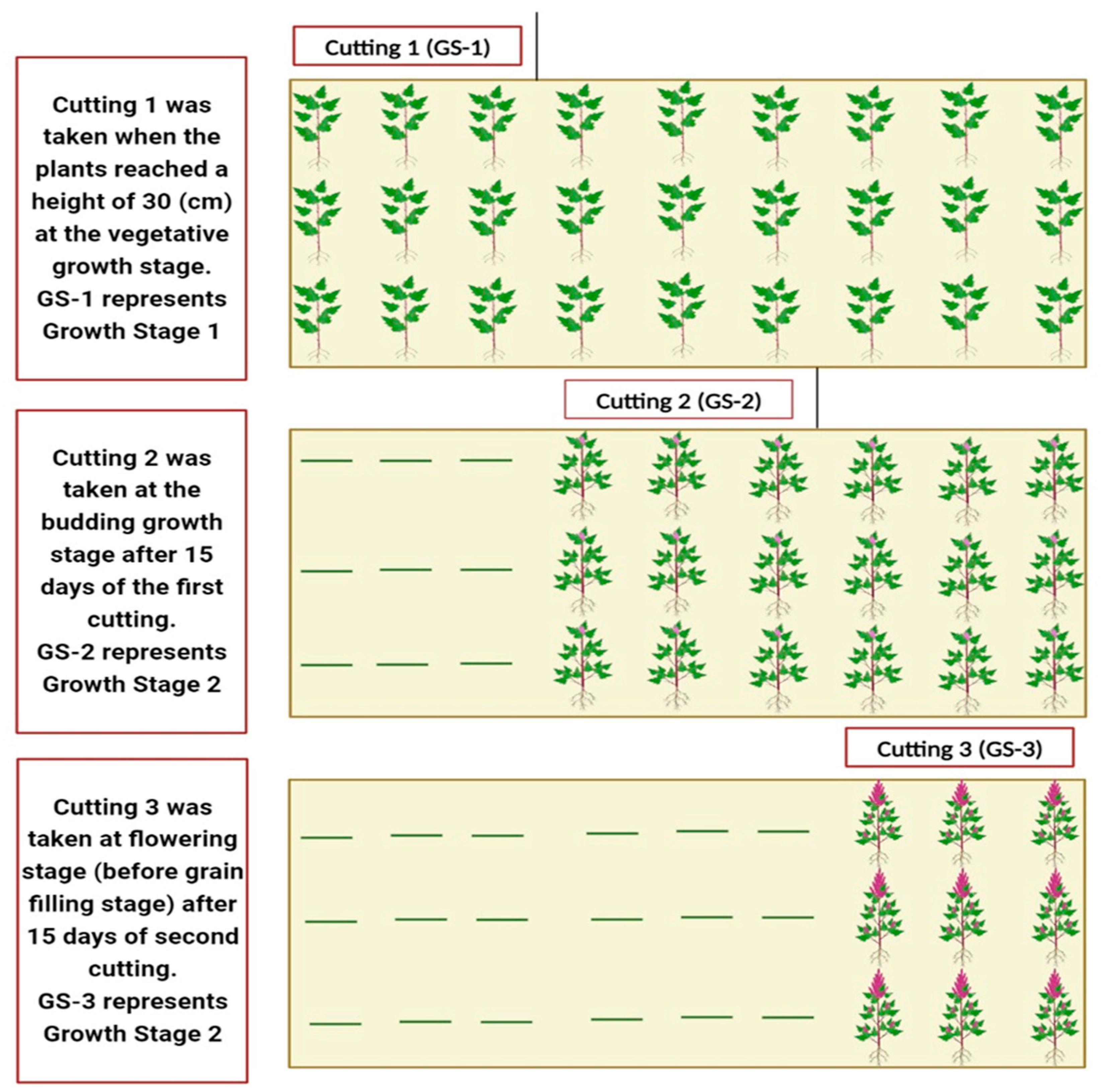
The current experiment was conducted for two consecutive years (i.e., 2018 to 2019 and 2019 to 2020) under the local climatic conditions of Faisalabad (31°25′7.3740″ N and 73°4′44.7924″ E; 186 m above sea level) at the Agronomy research area of the University of Agriculture, Faisalabad, Pakistan. The climate of Faisalabad is semi-arid and classified as very hot and humid in summer with cool and dry winters. Faisalabad receives an average annual rainfall of 375 mm and almost half of this falls during the monsoon season (i.e., July to August). A total of 10 accessions (R11, R126, R15, R24, R3, R30, R4, R9, and UAF7 originated from New Mexico, United States, and R45 originated from Chile) of Quinoa seeds (Figure 1) were collected from the department of crop physiology, University of Agriculture Faisalabad. Before sowing, the land was irrigated and prepared by two ploughings to a depth of 15 cm followed by planking to crush hard clods to smoothen the soil surface and preserve moisture in order to ensure maximum germination/emergence. The quinoa accessions for two growing seasons (i.e., year 1 and year 2) were sown on November 15th and November 20th, respectively. The seeds were sown manually using a hand dibbler (2–3 cm depth) with a 30 cm row-to-row distance. Plant-to-plant distance/within-row spacing was kept different, i.e., 21, 23, and 26 cm, and the data for different traits were recorded at three different cutting levels (i.e., cutting 1, cutting 2, and cutting 3) at different growth stages (vegetative growth stage, budding stage, and flowering stage) (Figure 2). The experimental layout was a split–split plot design under the randomized complete block (RCBD) arrangements with three replications, where levels of cutting were assigned in the main plot, levels of spacing were assigned in the subplot, and genotypes were assigned in the sub-subplots (Figure 1). The soil at the experimental site was a sandy loam and contained potassium (169 mg kg−1), nitrogen (0.4 g kg−1), phosphorus (8.1 mg kg−1), a pH of 7.82, and organic matter (0.74%). All agricultural practices such as irrigation (2 irrigations in first year and 1 in the second year due to heavy rains), fertilizer application (N:P:K: 75:50:50 kg ha−1), and weeding were conducted rigorously in a timely fashion. During the growing seasons, no major weather hazards such as insect/pest attacks occurred.

2.2. Measurements of Morphological and Quality Parameters

Data for different quality and morphological traits were recorded in three different levels of cutting (harvestings) at different growth stages. The first cutting was performed after the plants reached a height of 30 cm followed by cutting 2 and cutting 3- with 15-day intervals between each cutting. Five plants from each plot were selected randomly, and data were recorded for plant height (PH cm), leaf area (LA cm2), number of branches/plant (Br), number of leaves/plant (NoL), intermodal distance (ID cm), dry weight (DW g plant−1), and fresh weight (FW g plant−1). Fresh weight was immediately measured after each cutting using a weighing balance (Mhand, DJ-V-B). To measure dry weight, plants were transferred into paper bags, dried in the sun for 2 days, and then transferred to the oven for further drying at 65 ± 2 °C until a constant weight was obtained. After dry weight measurements, stem and leaves were separated and ground in a grinder machine, and data for fodder quality traits such as crude fat (CF %), crude protein (CP %), neutral detergent fiber (NDF %), acid detergent fiber (ADF %) [37], and moisture (Mois %) were recorded separately for both stems and leaves using a near-infrared (NIR) instrument (AgriNIR™) [38].

2.3. Statistical Analysis

To test the normality and homogeneity of variance, Shapiro–Wilk and Bartlett’s tests were used, respectively. Data were also checked for any outliers and multicollinearity among the variables before performing ANOVA. Data of all traits were subjected to split–split plot ANOVA to measure the main and interaction effects in each year separately (Supplementary Table S1). To analyze the overall effect and interactions of cutting (cut), spacing (space), genotype (gen), and year for all traits, a 4-way multivariate analysis of variance (MANOVA) was used to obtain a cumulative significance value based on Pillai’s trace test [39] using the model mentioned below:
Y = X b + e
where Y represents a response variable matrix of n × p, n represents total plot numbers, i.e., the combinations of different levels for cutting (c = 1, 2, 3), spacing (s = 1, 2, 3), genotypes (g = 1, 2, 10), and years (y = 1, 2), and p represents the total number of traits. Furthermore, X, b, and e represent n × m model matrix (as m = c × s × g), m × p coefficients model matrix, and n × p residuals model matrix, respectively. The estimated means for all treatments and traits were organized into rows and columns in a two-way table using the projected values from significant terms. Tukey’s multiple comparison test (p < 0.05) was undertaken to measure differences using means of genotypes and treatments. In order to identify the best combination of cut × space treatment to obtain the maximum benefits and the best performing genotypes, the MGIDI [40] was used with the help of the metan package:
M G I D I i = j = 1 f γ i j γ j 2 0.5
where MGIDIi represents multi-trait genotype-ideotype distance index for the ith row/genotype/treatment; ij represents the ith score row/genotype/treatment in the j th factor (i = 1; 2;…; g; j =1; 2;…; f), with g and f being the number of rows/genotypes/treatments and factors, respectively; and j represents the ideotype j th score. The combinations that depict the lowest MGIDI will be adjacent to the ideotype and, thus, exhibit preferred values for all measured traits. Selection intensity (SI) of  ~20% for main effects and 10% for interactions was considered for selection differential for all traits. Based on the ideotype concept, all the traits were assigned a value between 0–100, where 0 represents a least-valued trait, and 100 represents a most-desired trait. In this study, LADF, LNDF, SADF, and SNDF were selected as traits in which a decreased value was more desirable, while for the rest of the traits, an increased value was desirable. Moreover, weights were also added to traits to provide differential importance to each trait. The morphological traits were given a value of 0.5, whereas the quality parameters were assigned a value of 1 to indicate that, during selection of genotypes/cutting/spacing, these traits will be considered first, followed by the morphological traits.
All the data manipulation and analyses were carried out using R software (version 4.2.2). Correlation matrix between different morphological and quality traits along with all treatment combinations were generated and plotted using qgraph package, bar-graphs, and a climograph for weather data (Figure 3), and other figures were drawn using the ggplot2, dplyr, patchwork, plotly, and metan packages in R software.

3. Results

MANOVA results revealed that all the main effects (genotypes, cut, space, and years) showed significant (p < 0.05 & 0.01) differences. All the possible two-way interactions studied between the main effects were found significant except space × year, indicating that the response of the genotypes was influenced by cutting, spacing, and year effects. As for the three-way interactions, only cut × space × gen and cut × gen × year were found significant, while the four-way interaction was found non-significant (Supplementary Table S2).

3.1. Climatic Conditions

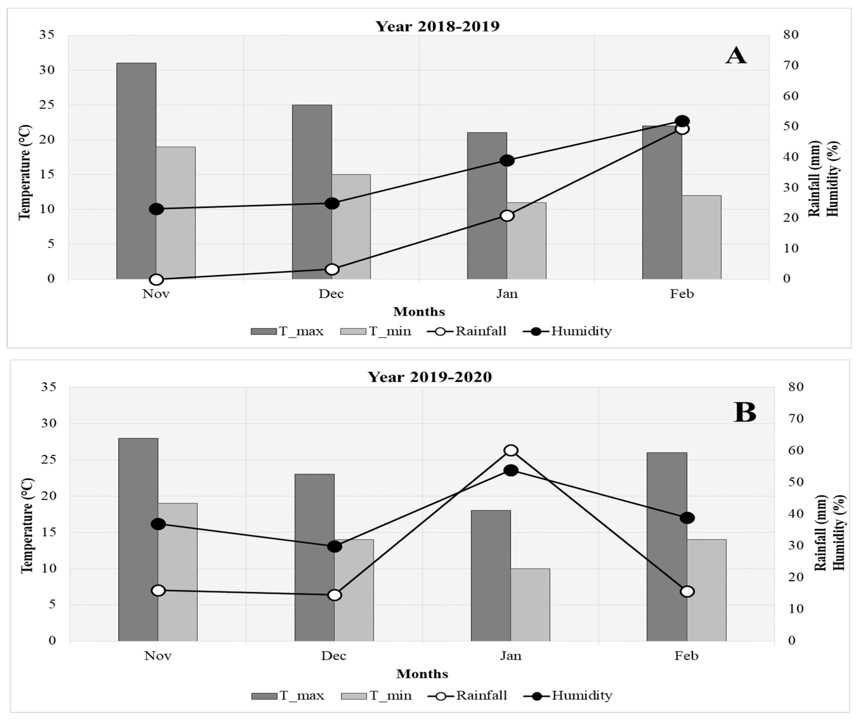
The maximum and minimum temperature during the first growing season was recorded 19 and 11 °C in November and January, respectively. In the second growing season, the maximum (19 °C) and minimum (10 °C) temperature was recorded in November and January, respectively (Figure 3). The average rainfall per year (last 55 years) in Faisalabad in November, December, January, and February has recorded 2.9, 3.1, 16.9, and 26.3 mm. During the first growing season, 0, 3.3, 20.9, and 49.4 mm of average rainfall was recorded in November, December, January, and February, respectively. While in the second growing season, the average rainfall in all months (except February) remained much higher than in the first growing season. During the second growing season, 16.1, 14.6, 60.3, and 15.7 mm of rainfall was recorded in November, December, January, and February, respectively. Moreover, the same pattern was observed for relative humidity, where, during the first growing season, it was 23% in November, 25% in December, 39% in January, and 52% in February, while in the second growing season, humidity remained at 37% in November, 30% in December, 54% in January, and 39% in February.

3.2. Morphological and Forage Quality Traits of Quinoa Genotypes

Bar graphs (mean values) of quality and morphological traits are presented along with Tukey’s mean comparison test results (Supplementary Figure S1). The year effect for most morphological traits was significant. PH, NoL, Br, FW, and DW showed significantly higher values at cutting level 3 for all the genotypes than at C1 and C2 levels, while for LA and ID, no significant effects of cutting, spacing, and year were recorded. S2 (23 cm) was more effective for morphological traits than S1 (21 cm) and S3 (26 cm) (Supplementary Figure S1).
Among leaf quality parameters, all the quality traits were stable across years except LNDF and LCF. The concentrations of all quality parameters increased with an increase in growing time, and hence, concentrations at cutting level 1 were lower than at cutting levels 2 and 3. Furthermore, S2 was more effective for all quality parameters (except LNDF) compared with S1 and S3 (Supplementary Figure S2). Stem quality traits also showed a similar pattern, where significant differences were observed in spacing and year for all traits except SADF (Supplementary Figure S3). However, SCP increased with an increase in growth time, i.e., from cutting 1 to cutting 2 but decreased at cutting 3 (Supplementary Figure S2A). SCF, SADF, SNDF, and SMois slightly increased at cutting level 3 compared to cutting level 2 (Supplementary Figure S2B–E).

3.3. MGIDI Index Selection

Keeping in view the significance and importance of factors, the MGIDI was calculated for (i) cut × space to identify the best possible combination for quinoa and (ii) genotype selection and to identify the best genotypes that performed ideally at all levels of cutting and spacing in both years. Based on the studied pattern, traits were grouped into the same factor.

3.3.1. Selection of Best Application combination (Cut × Space) to Obtain the Maximum Desired Gains

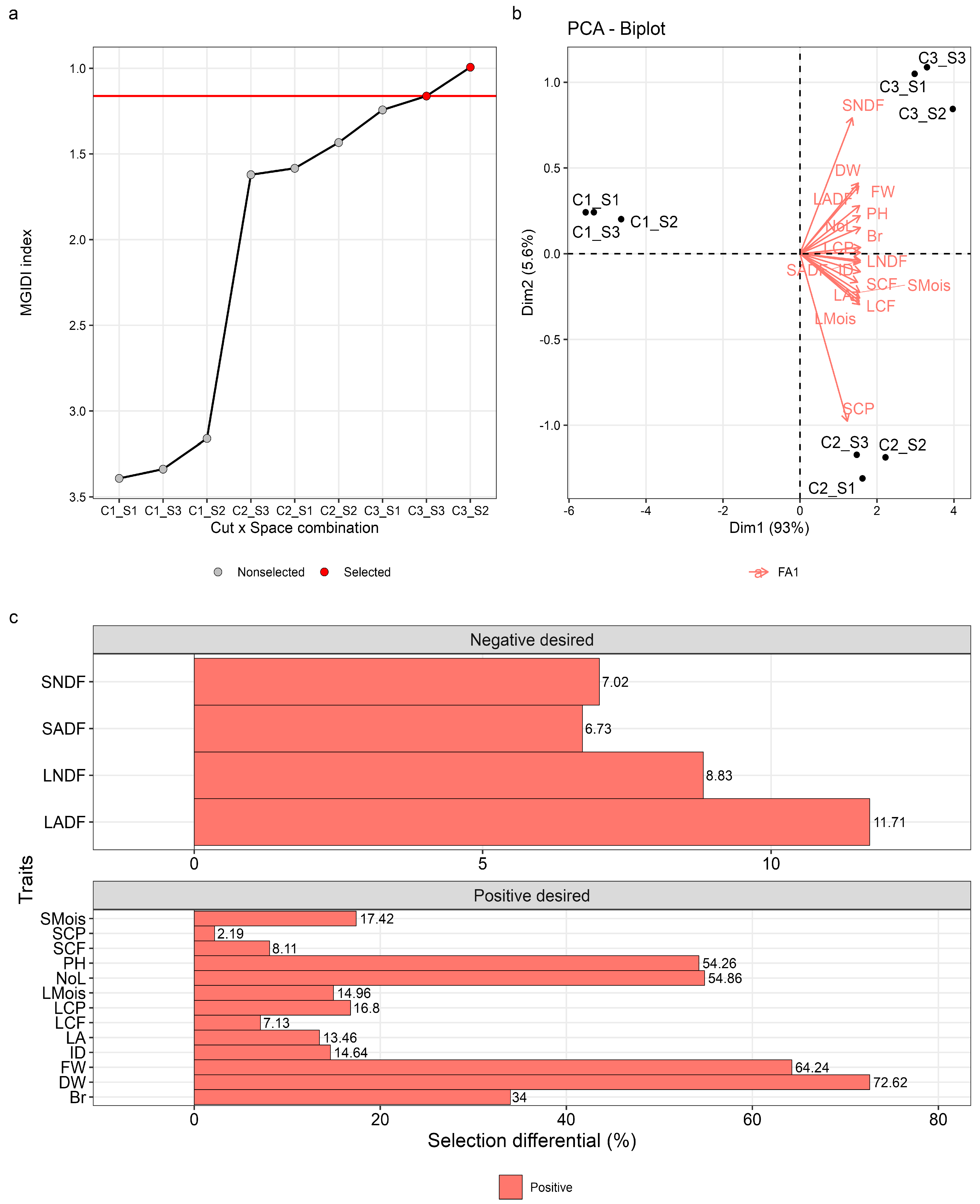
The MGIDI was computed to rank the treatment combination (cut × space) based on the desired values of each trait. The factor analysis grouped all the studied traits into single factors (FA1) based on their similar pattern as follows (Table 1). Combination ranking according to the MGIDI showed that cutting level 3 combined with spacing level 2 (23 cm) was more effective for achieving the desired results, followed by C3-S3 (Supplementary Figure S1). The computed MGIDI displayed the desired selection differentials (SDs) for 13 out of 17 studied traits, which means that our goal for the selected 13 traits was achieved (Figure 4). The SDs quantify the population’s mean trait value alterations between pre-selection and post-selection. The SD for the traits with less-desired values ranged from 6.73% (SADF) to 11.7% (LADF). The SD for the traits with more highly desired values ranged from 2.19% (SCP) to 72.6% (DW). Overall, the computed MGIDI index displayed lower total gain, i.e., 28.8% and 8.57% for the traits that tended to increase and decrease, respectively. The positive SD observed for productive traits was mainly due to C3-S2 and C3-S3, indicating that a combination of C3 with S2 would be more fruitful for obtaining the maximum desired gain for the quinoa genotypes.

3.3.2. Selection of Best Performing Genotypes

In the significant factor analysis of genotype, 17 traits were grouped into five factors (FA1-5) (Table 2). The MGIDI provided a total SD of 5.31% for traits that tended to increase and −3.43% for traits that tended to decrease. The SDs calculated with these genotypes were desired for a total of 15 traits out of 17. The SD ranged from −8.83% (LADF) to 1.70% (SNDF) for traits desired with low values and from −1.61% (ID) to 15.9% (FW) for traits desired with high values. Overall, all the genotypes performed better in the second growing season, with R9 and R3 ranked as the most suitable genotypes. Both genotypes showed maximum contribution in FA1 and FA4, mainly relying on quality-related traits (Figure 5). The selected genotypes were then used to compute the SD. The strengths and weaknesses plot and PCA (Figure 5b,c) showed that the selected genotype’s strengths were mostly associated with FA1 and FA4, i.e., higher values for most of the morphological and quality traits compared to the other genotypes. Factors that contributed the most and least were drawn at the center and edges of the plot, respectively.

3.4. Correlation Analysis

Forage biomass and quality depend on the relationship among the traits that directly contribute to quality and yield. In this study, correlation analysis revealed moderate (p < 0.05) and high (p < 0.01) significant positive correlations among the studied traits in both years under all levels of cutting and spacing, but some traits also showed negative correlations (Supplementary Tables S3–S8).

3.4.1. Correlation Analysis of Cutting Level 1 in Both Years

In the first year under cutting and spacing level 1, PH_C1S1 had highly and moderately significant positive correlations with Br_C1S1 (r = 0.915), NoL_C1S1 (r = 0.684), and FW_C1S1 (r = 0.660), and NoL_C1S1 was positively correlated with FW_C1S1 (r = 0.881) and DW_C1S1 (r = 0.770) (Supplementary Figure S4A subplot a (yellow circles)). Furthermore, under cutting level 1 and spacing level 2, PH_C1S2, LA_C1S2, and FW_C1S2 had highly significant positive correlations with LCF_C1S2 (r = 0.816), FW_C1S2 (r = 0.793), and DW_C1S2 (r = 0.931), respectively (Supplementary Figure S4A subplot a (green circles)). Additionally, under cutting level 1 and spacing level 3, PH_C1S3 had a highly significant positive correlation with LA_C1S3 (r = 0.825). NoL_C1S3, LA_C1S3, ID_C1S3, DW_C1S3, and LCP_C1S3 had moderately significant positive correlations with FW__C1S3 (r = 0.585), LCP__C1S3 (r = 0.566), DW__C1S3 (r = 0.461), LCP__C1S3 (r = 0.540), and SCF__C1S3 (r = 0.521), respectively (Supplementary Figure S4A subplot a (blue circles)).
In the second year, under cutting and spacing level 1, PH_C1S1, Br_C1S1, FW_C1S1, and SCP_C1S1 had highly significant positive correlations with Br_C1S1 (r = 0.903), FW_C1S1 (r = 0.878), DW_C1S1 (r = 0.793), and SCF_C1S1 (r = 0.777), respectively (Supplementary Figure S4A subplot b (yellow circles)). Similarly, under cutting level 1 and spacing level 2, PH_C1S2 was highly positively correlated with Br_C1S2 (r = 0.795) and FW_C1S2 (r = 0.823). LA_C1S2 and LADF_C1S2 were positively correlated with SCF_C1S2 (r = 0.790) and LNDF_C1S2 (r = 0.940), respectively (Supplementary Figure S4A subplot b). Furthermore, under cutting level 1 and spacing level 3, PH_C1S3 had highly significant positive correlations with Br_C1S3 (r = 0.723), ID_C1S3 (r = 0.849), and FW_C1S3 (r = 0.846). ID_C1S3 and FW_C1S3 had highly significant positive correlations with FW_C1S3 (r = 0.843) and DW_C1S3 (r = 0.774), respectively (Supplementary Figure S4A subplot b).

3.4.2. Correlation Analysis of Cutting Level 2 in Both Years

In the first year, under cutting level 2 and spacing level 1, NoL_C2S1, LA_C2S1, Br_C2S1, FW_C2S1, and LADF_C2S1 had highly significant positive correlations with Br_C2S1 (r = 0.766), LCP_C2S1 (r = 0.796), FW_C2S1 (r = 0.807), DW_C2S1 (r = 0.980), and LNDF_C2S1 (r = 0.881), respectively (Supplementary Figure S4B subplot a). Additionally, under cutting and spacing level 2, FW_C2S2 had a highly significant positive correlation with DW_C2S2 (r = 0.969) (Supplementary Figure S4B subplot a), and under cutting level 2 and spacing level 3, NoL_C2S3 had moderately significant positive correlations with Br_C2S3 (r = 0.682), FW_C2S3 (r = 0.764), and DW_C2S3 (r = 0.763). FW_C2S3 and LADF_C2S3 were highly positively correlated with DW_C2S3 (r = 0.986) and LNDF_C2S3 (r = 0.906) (Supplementary Figure S4B subplot a).
In the second year, under cutting level 2 and spacing level 1, NoL_C2S1 was highly positively correlated with FW_C2S1 (r = 0.904) and DW_C2S1 (r = 0.851). ID_C2S1 a had highly positive correlation with LCP_C2S1 (r = 0.810), and FW_C2S1 had a highly positive correlation with DW_C2S1 (r = 0.980) and a moderately positively correlation with Br_C2S1 (r = 0.750). DW_C2S1 also showed a moderate positive correlation with Br_C2S1 (r = 0.725). ID_C2S1, FW_C2S1, and LADF_C2S1 had positive correlations with LCP_C2S1 (r = 0.810), DW_C2S1 (r = 0.980), and LNDF_C2S1 (r = 0.826), respectively. LCP_C2S1 and LA_C2S1 were moderately positively correlated with SCP_C2S1 (r = 0.743) and SCF_C2S1 (r = 0.661), respectively (Supplementary Figure S4B subplot b). Similarly, under cutting level and spacing level 2, NoL_C2S2, FW_C2S2, and DW_C2S2 had highly significant positive correlations with Br_C2S2 (r = 0.808), DW_C2S2 (r = 0.839), and SADF_C2S2 (r = 0.880) (Supplementary Figure S4B subplot b). Under cutting level 2 and spacing level 3, NoL_C2S3, ID_C2S3, FW_C2S3, and LADF_C2S3 had highly significant positive correlations with FW_C2S3 (r = 0.775), SMois_C2S3 (r = 0.798), DW_C2S3 (r = 0.959), and LNDF_C2S3 (r = 0.821), respectively (Supplementary Figure S4B subplot b).

3.4.3. Correlation Analysis of Cutting Level 3 in Both Years

In the first year, under cutting level 3 and spacing level 1, PH_C3S1 was highly positively correlated with Br_C3S1 (r = 0.767) and ID_C3S1 (r = 0.853); NoL_C3S1 had highly significant positive correlations with Br_C3S1 (r = 0.793), ID_ C3S1 (r = 0.823), FW_ C3S1 (r = 0.852), and DW_ C3S1 (r = 0.835); Br_C3S1 was highly positively correlated with FW_C3S1 (r = 0.775) and DW_C3S1 (r = 0.785); and LADF_C3S1 had a highly positive correlation with LNDF_C3S1 (r = 0.767) (Supplementary Figure S4C subplot a). Similarly, under cutting level 3 and spacing level 2, PH_C3S2, NoL_C3S2, Br_C3S2, ID_C3S2, and FW_C3S2 had highly significant positive correlations with ID_C3S2 (r = 0.860), FW_C3S2 (r = 0.828), DW_C3S2 (r = 0.808), FW_C3S2 (r = 0.773), and DW_C3S2 (r = 0.952), respectively (Supplementary Figure S4C subplot a). Moreover, under cutting and spacing level 3, PH_C3S3, NoL_C3S3, and ID_C3S3 had highly significant positive correlations with ID_C3S3 (r = 0.888), FW_C3S3 (r = 0.871), and SCF_C3S3 (r = 0.813), respectively (Supplementary Figure S4C subplot a).
In the second year, under cutting level 3 and spacing level 1, NoL_C3S1 showed highly significant positive correlations with Br_C3S1 (r = 0.904), ID_C3S1 (r = 0.779), FW_C3S1 (r = 0.894), and DW_C3S1 (r = 0.910); Br_C3S1 had highly significant positive correlations with ID_C3S1 (r = 0.796), FW_C3S1 (r = 0.848), and DW_C3S1 (r = 0.835); ID_C3S1 was highly positively correlated with FW_C3S1 (r = 0.813) and DW_C3S1 (r = 0.844); and FW_C3S1 had a highly significant positive correlation with DW_C3S1 (r = 0.989) (Supplementary Figure S4C subplot b). In addition, under cutting level 3 and spacing level 2, PH_C3S2 had moderately significant positive correlations with NoL_C3S2 (r = 0.635), Br_C3S2 (r = 0.692), and DW_C3S2 (0.645), while NoL_C3S2 was highly positively correlated with FW_C3S2 (r = 0.872) and DW_C3S2 (r = 0.831). Br_C3S2 had highly significant positive correlations with ID_C3S2 (r = 0.836) and DW_C3S2 (r = 0.776). Moreover, FW_C3S2 and LADF_C3S2 also had highly significant positive correlations with DW_C3S2 (r = 0.988) and LNDF_C3S2 (r = 0.860), respectively (Supplementary Figure S4C subplot b). Under cutting and spacing level 3, Nol_C3S3 had highly significant positive correlations with Br_C3S3 (r = 0.769), FW_C3S3 (r = 0.895), and DW_C3S3 (r = 0.903); Br_C3S3 had positive correlations with FW_C3S3 (r = 0.854) and DW_C3S3 (r = 0.853); and FW_C3S3 had a highly significant positive correlation with DW_C3S3 (r = 0.998) (Supplementary Figure S4C subplot b).
An increase in biomass resulted in the degradation of anti-nutritional quality traits (ADF and NDF). Biomass-related traits like PH, NoL, LA, Br, FW, and DW showed highly and moderately significant negative correlations with LADF and LNDF, ranging from r = −0.501 to −0.935 in both years under all levels of cutting and spacing (Supplementary Figure S4A–C subplot a-b-c).

3.5. Comparison with Oat

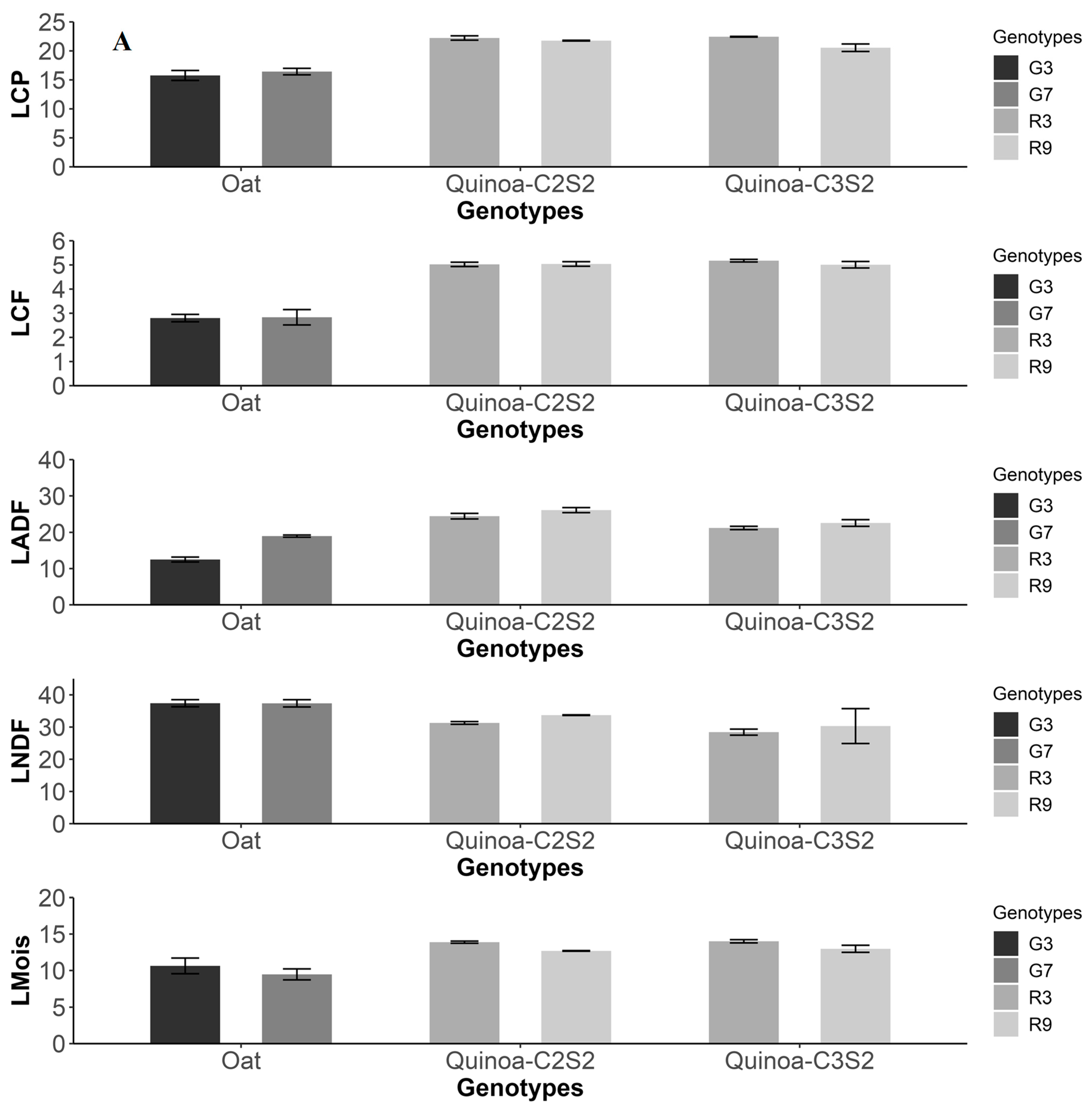
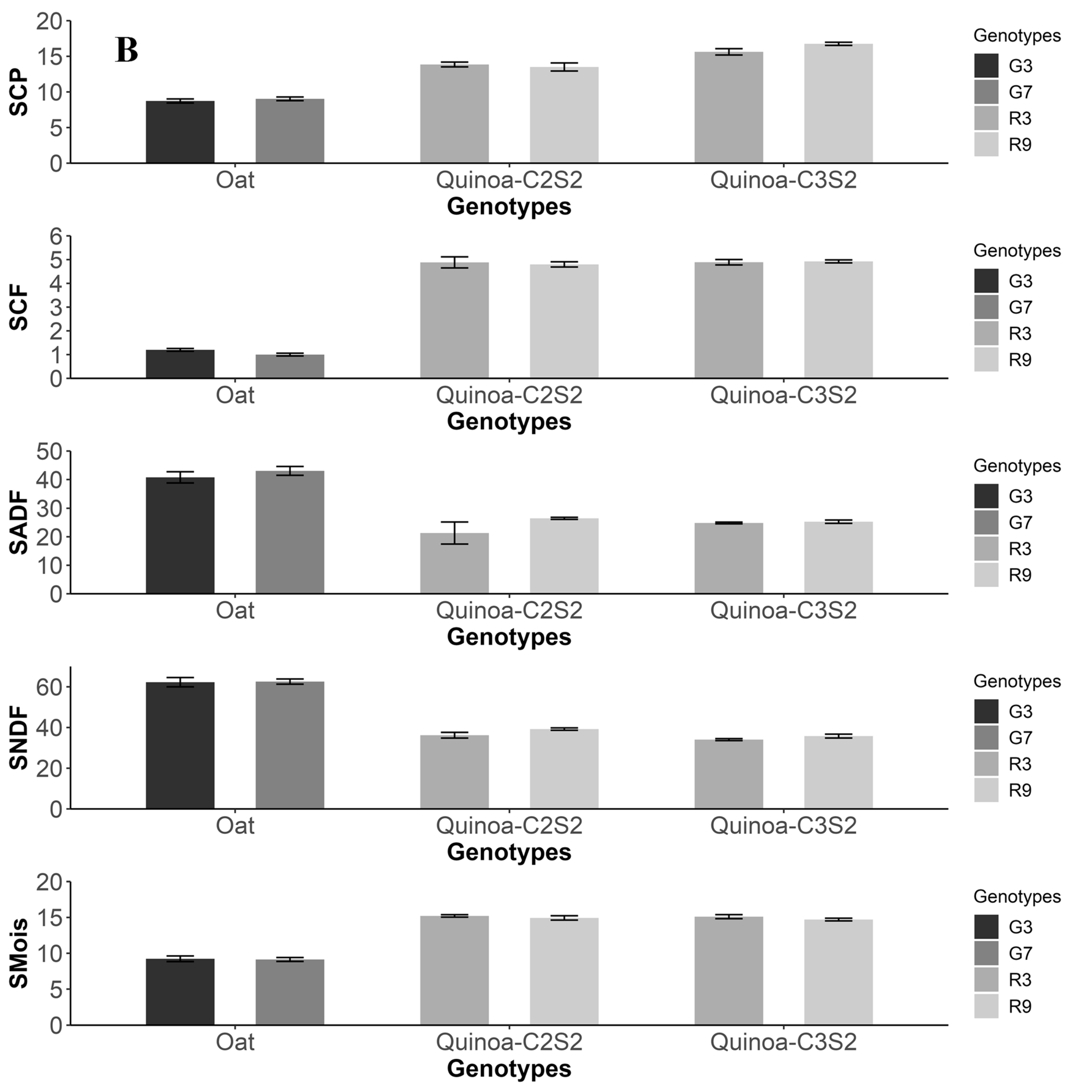
The quality traits of selected quinoa genotypes (R3 and R9) were compared with oat genotypes (G3 and G7). Quinoa genotypes at cutting level 2 and 3 under spacing level 2 (23 cm) were compared with oat quality parameters. Our results revealed that the CP and CF contents of quinoa in leaves and stems were significantly higher than those of oat (Figure 6A,B). In quinoa leaves, NDF (LNDF) was significantly lower at both cuttings than in oat accessions, while ADF (LADF) was slightly higher at both cuttings than in oat (Figure 6A). In stem, however, quinoa showed desirable results as the levels of both SADF and SNDF were significantly lower than oat accessions under both cutting levels (Figure 6B). Comparing the forage quality characteristics of quinoa and oat revealed low fiber (ADF and NDF) and high crude protein and fat (CP and CF) levels in quinoa, highlighting the importance of further research into this species.

4. Discussion

4.1. Environmental Factors Markedly Influenced Morphological and Forage Quality Traits of Quinoa in Both Years

Climatic factors like air temperature, rainfall, and humidity are known to have significant effects on quinoa growth and biomass production. Quinoa has already developed resistance to various abiotic factors and can resist a broad range of air temperature ranging from −8 to 35 °C [41]. The optimal temperature for better quinoa growth has been reported as 20 °C [42]. In present investigation, we also perceived the effects of the abovementioned climatic factors: in the second growing season, the quinoa gained more biomass in terms of PH, NoL, and Br compared to the first growing season. The average temperature in the second growing season in all months was closer to the quinoa optimal temperature compared to the first growing season and therefore resulted in more FW and DW (Supplementary Figure S1F,G). Quinoa can grow relatively well in humidity ranging from 40% to 88% [43]. In the second growing season, the relative humidity in all growing months was more stable and favorable for quinoa growth compared with the first growing season (Figure 3). This stability and increase in relative humidity in the second growing season were mainly due to higher rainfall across all the growing months compared with the first growing season (Figure 3). Thus, the effect of these climatic factors on quinoa growth can be clearly seen from the outcomes of the present investigation where the year effect was highly significant (p < 0.05) on most morphological traits except for LA and ID. In addition to biomass, forage quality is also directly associated with plant growth, nutrients in the tissues, community composition, and forage digestibility. In our investigation, we observed a significant (p < 0.05) year effect on forage quality parameters in both leaves and stems. During the second growing season, LCP, SCP, and SCF levels increased in stems and leaves compared with the first growing season (Supplementary Figure S2A). Moreover, LCP, LCF, SCP, and SCF levels increased with the increase in forage biomass, and these findings were consistent with those of a two-year field experiment conducted in [44].

4.2. Effect of Different Treatments on Morphological and Quality Traits of Quinoa

In addition to climatic factors, various other practices such as different levels of cuttings and plant-to-plant spacing also affect quinoa biomass and quality. Cuttings at different growth stages significantly affect crop (oat, alfalfa, canola, and millet) biomass and forage quality [45,46,47,48]. However, very limited research data are available on the effect of cuttings at different growth stages of quinoa. Yilmaz et al. [49] evaluated the effect of cuttings at three different stages to determine the quality and forage yield of quinoa. Their results revealed that different cutting levels had significant effects on dry forage yield and other morphological and forage quality parameters. In our study, we also observed the same effects of cuttings on quinoa morphological and quality traits. Different cutting levels significantly affected PH, NoL, Br, FW, DW, LCP, SCP, and SCF, and maximum biomass was recorded at cutting level 3 in both years (Supplementary Figure S1A–G). Furthermore, LA and ID showed mixed responses in which a few genotypes like R4, R45, and UAF performed better at cutting level 2 rather than cutting level 3. In the case of quality, the concentrations of quality traits such as LCP, LCF, SCP, SCF, LADF, LNDF, SADF, SNDF, LMois, and SMois remained lower at cutting level 1, increased with the increase in growth time, and slightly varied between cutting levels 2 and 3 (Supplementary Figure S2A–E). Our results were in agreement with multi-field trials under two cutting levels, in which maximum biomass and quality were produced at cutting level 2 rather than cutting level 1 [50].
In addition to cutting levels, plant-to-plant distance (spacing level) is another important factor affecting quinoa biomass and quality [35,51]. Finding the appropriate plant-to-plant distance for quinoa cultivation is a major challenge as a slight change in plant-to-plant distance can result in large variations in PH, NoL, Br, CP, CF, ADF, and NDF. Zulkadir [36] planted quinoa variety Q-52 using three different spacing levels, i.e., 20, 40, and 60 cm to determine the most appropriate plant-to-plant distance to gain maximum biomass production. Zulkadir [36] identified 20 cm as the most appropriate spacing level to gain maximum grain yield and biological yield followed by 40 and 60 cm, respectively. Similarly, Reddy et al. [52] also planted quinoa genotypes with three different spacing levels (20 × 10 cm, 25 × 10 cm, and 30 × 10 cm) along with nitrogen (N) levels to evaluate the effects of the given treatments on yield. They reported 30 × 10 cm + 25% N as the most appropriate treatment to gain maximum stover yield and seed yield, while 20 × 10 cm + 25% N was reported as the most appropriate to gain the maximum B:C ratio, net returns, and gross returns. In the present study, three different spacing levels, viz., 21, 23, and 26 cm were used to determine the appropriate spacing level to achieve maximum biomass and forage quality. Just like cutting, different levels of spacing also showed significant effects on quinoa biomass and quality. The maximum biomass in terms of PH, NoL, Br, FW, and DW was observed under spacing level two (S2), i.e., 23 cm followed by S1 (21 cm) and S3 (26 cm) (Supplementary Figure S1A–G). However, no significant effects of spacing levels were observed on LA and ID. Similarly, S2 was also more effective for quality parameters like CP, CF, NDF, and ADF in both leaves and stems except for NDF in leaves and ADF in stems (Supplementary Figure S1A–E). These findings were in agreement with the findings reported by Asher et al. [35], Temel and Yolcu [53], TEMEL and KESKIN [54], and Sief et al. [55].

4.3. Treatment Combination and Genotypes Selection Using the MGIDI

The selection of suitable genotypes has always been a challenge for plant breeders. Most plant breeders use classical stability indexes like deviation from regression, regression, and mean to select the most stable genotype [56,57]. However, these statistical tools are insufficient to detect the weaknesses and strengths of genotypes and to select individuals with desired average performance and stability [58]. The MGIDI is a sophisticated quantitative genetic technique used to exploit desired accessions in all crop species [59] and is free from multi-collinearity problems [60]. In the current study, the MGIDI was computed for the best treatment combination (cut × space) and for the selection of suitable genotypes by grouping the studied traits into the same factor. According to the MGIDI results, cutting level 3 in combination with spacing level 2 (23 cm) was more effective in achieving the maximum biomass and quality of quinoa than other treatments (Figure 4a). Moreover, among all the genotypes, R9 and R3 gathered the desired mean performance and stability of several traits such as PH, NoL, Br, FW, DW, LCP, LCF, LADF, LMois, SCP, SCF, SADF, and SMois (Figure 4c and Figure 5a–d). Moreover, the selection of appropriate quinoa genotypes aligned with sustainable agricultural principles has several potential benefits. Firstly, it can contribute to food security by improving crop yields and nutritional quality. Secondly, the identification of genotypes with resource-efficient traits can promote sustainable resource management, reducing water, fertilizer, and pesticide use. Additionally, by selecting genotypes with resistance to pests and diseases, farmers can reduce the need for chemical interventions, thus minimizing environmental impacts. Furthermore, the adaptability of genotypes to changing climatic conditions can enhance the resilience of agricultural systems.
Furthermore, correlation analysis revealed a highly significant and moderately significant positive correlation among the studied traits under all levels of cutting and spacing in both years. Among all productive traits, PH and NoL showed a highly significant positive correlation with most of the traits that directly contribute to biomass such as LA, Br, ID, FW, and DW. An increase in PH is directly associated with an increase in NoL [61,62], LA [63,64], FW [65,66], and DW [67,68]. Similar results were seen for quality traits in which an increase in the productive traits such as PH, LA, ID, and DW led to increasing LCF, LCP, and SCF (Supplementary Figure S4A,B subplot a-b). Forage digestibility (energy) depends on the levels of anti-quality traits such as ADF and NDF [69]. ADF is a fiber portion that consists of lignin and cellulose. ADF is mainly associated with the digestibility of forage and is, therefore, necessary to compute forage net energy (NE) or total digestible nutrients (TDN) for silage, haylage, and hay [70]. On the other hand, NDF is the most common measure of fiber used for animal feed analysis but does not represent a unique class of chemical compounds. NDF measures most of the structural components of plant cells such as cellulose, hemicellulose, and lignin but not pectin [71]. In general, both ADF and NDF values increased as the forage matured. Forages with low ADF and NDF levels are usually higher in energy [72]. LADF had a highly positive significant correlation with LNDF (Supplementary Figure S4A–C subplot a-b), indicating that an increase in NDF level is directly associated with an increase in ADF. Furthermore, increases in PH, NoL, LA, FW, and DW decreased ADF and NDF levels in both leaves and stems (Supplementary Figure S4A–C subplot a-b-c). These findings were consistent with other findings, in which an increase in forage yield resulted in increases in CP and CF and decreases in NDF and ADF [43,73,74,75].
Oat (Avena sativa L.) is commonly used as an annual forage crop in irrigated and rain-fed areas worldwide. Oat has great biomass production with high forage quality [76,77]. Therefore, to further analyze the fitness of quinoa as potential forage, we compared the quality traits of two selected genotypes (R3 and R9) with two oat accessions (G3 and G7). Quinoa had a greater amount of crude protein and crude fat (CP and CF) in both leaves and stems compared to oat (Figure 6A). The concentrations of anti-quality traits such as ADF and NDF were lower in quinoa leaves (except for LADF) and stems compared to oat (Figure 6B). Furthermore, this comparison revealed the latent potential of quinoa species as an alternative source of high-quality forage.

5. Conclusions

Our findings reveal that quinoa biomass production and quality traits are greatly influenced by environmental factors. Optimum air temperature and relative humidity are essential for the growth and development of quinoa to obtain maximum biomass and high-quality forage. In the second growing season, the environmental conditions were more favorable for quinoa than the first growing season and therefore showed remarkable growth in the second season. In addition to environmental factors, other practices such as different cutting and spacing levels also affected quinoa growth in terms of PH, NoL, Br, FW, and DW. Under all cuttings and spacing levels, cutting level 3 in combination with spacing level 2 (23 cm) was more effective for quinoa biomass and quality traits across both years. In the current study, the selected quinoa genotypes (R3 and R9) using MGIDI, had shown significant improvement in both morphological and quality traits. Furthermore, morphological traits such as PH, NoL, LA, FW, and DW showed moderately significant negative correlations with anti-quality traits, indicating that an increase in biomass can reduce concentrations of anti-nutritional quality traits to enhance the forage digestibility. The selected quinoa genotypes were then compared to the quality parameters of oat accessions. The comparison revealed that quinoa has more CP and CF and low NDF in both leaves and stems than oat. Overall, the findings indicated that quinoa has latent potential as an alternative forage to fulfill the forage demand gap in Pakistan.

Supplementary Materials

The following supporting information can be downloaded at https://www.mdpi.com/article/10.3390/su151411446/s1. Figure S1: Morphological Traits of 10 Quinoa genotypes studied during two years at different cutting and spacing levels; Figure S2: Leaf Quality Traits of 10 Quinoa genotypes studied during two years at different cutting and spacing levels; Figure S3: Stem Quality Traits of 10 Quinoa genotypes studied during two years at different cutting and spacing levels; Figure S4: Correlations among matrixes of various traits under different cuts and spacing levels; Table S1: Split-Split Plot ANOVA of both Years (2018–2019 & 2019–2020) for all Traits of 10 Quinoa Genotypes tested at different Cuttings and Spacing Levels; Table S2: MANOVA results of 17 traits f 10 Quinoa genotypes evaluated at cutting and spacing levels for two years. Pillai’s trace test was used to get a cumulative significance value for the studied main effects and interactions; Table S3: Correlation Matrix for the cutting1 × spacing 1, 2, and 3 during first growing season (year 1) for all the 17 traits of 10 Quinoa genotypes; Table S4: Correlation Matrix for the cutting 2 × spacing 1, 2, and 3 during first growing season (year 1) for all the 17 traits of 10 Quinoa genotypes; Table S5: Correlation Matrix for the cutting 3 × spacing 1, 2, and 3 during first growing season (year 1) for all the 17 traits of 10 Quinoa genotypes; Table S6: Correlation Matrix for the cutting 1 × spacing 1, 2, and 3 during second growing season (year 2) for all the 17 traits of 10 Quinoa genotypes; Table S7: Correlation Matrix for the cutting 2 × spacing 1, 2, and 3 during second growing season (year 2) for all the 17 traits of 10 Quinoa genotypes; Table S8: Correlation Matrix for the cutting 3 × spacing 1, 2, and 3 during second growing season (year 2) for all the 17 traits of 10 Quinoa genotypes.

Author Contributions

Conceptualization, A.B., M.G. and S.R.A.; methodology, S.R.A., A.B. and M.G.; software and statistical analysis, M.G., A.B. and S.R.A.; investigation, S.R.A., A.B., Z.A., Z.K., I.I., S.P. and M.S.T.; data curation, M.G., A.B., D.K.Y.T. and S.R.A.; writing—original draft preparation, S.R.A., M.G., A.B., Z.A., I.I., Z.K., S.P., N.G. and M.S.T.; writing—review and editing, S.R.A., M.G., A.B., K.R.H., H.F.A. and D.K.Y.T.; supervision, A.B.; All authors have read and agreed to the published version of the manuscript.

Funding

This research was funded by the Institutional Fund Project under grant no. IFPIP: 287-130-1443. The authors gratefully acknowledge the technical and financial support provided by the Ministry of Education and King Abdulaziz University, DSR, Jeddah, Saudi Arabia.

Institutional Review Board Statement

Not applicable.

Informed Consent Statement

Not applicable.

Data Availability Statement

Data are contained within the article.

Acknowledgments

This research was funded by the Institutional Fund Project under grant no. IFPIP: 287-130-1443. The authors gratefully acknowledge the technical and financial support provided by the Ministry of Education and King Abdulaziz University, DSR, Jeddah, Saudi Arabia.

Conflicts of Interest

The authors declare no conflict of interest.

References

  1. Ortiz-Bobea, A.; Ault, T.R.; Carrillo, C.M.; Chambers, R.G.; Lobell, D.B. Anthropogenic climate change has slowed global agricultural productivity growth. Nat. Clim. Chang. 2021, 11, 306–312. [Google Scholar] [CrossRef]
  2. Steensland, A. 2019 Global Agricultural Productivity Report: Productivity Growth for Sustainable Diets and More (Virginia Tech, 2019). Available online: http://hdl.handle.net/10919/96429 (accessed on 16 October 2019).
  3. Chambers, R.G.; Pieralli, S.; Sheng, Y. The millennium droughts and Australian agricultural productivity performance: A nonparametric analysis. Am. J. Agric. Econ. 2020, 102, 1383–1403. [Google Scholar] [CrossRef]
  4. Gil, J. Global climate sensitivity of cropping frequency and yields. Nat. Food 2023, 4, 114–123. [Google Scholar] [CrossRef]
  5. Navarro-Racines, C.; Tarapues, J.; Thornton, P.; Jarvis, A.; Ramirez-Villegas, J. High-resolution and bias-corrected CMIP5 projections for climate change impact assessments. Sci. Data 2020, 7, 7–15. [Google Scholar] [CrossRef] [Green Version]
  6. Fu, G.; Wang, J.; Li, S. Response of forage nutritional quality to climate change and human activities in alpine grasslands. Sci. Total Environ. 2022, 845, 157552. [Google Scholar] [CrossRef]
  7. Wijerathna-Yapa, A.; Pathirana, R. Sustainable Agro-Food Systems for Addressing Climate Change and Food Security. Agriculture 2022, 12, 1554. [Google Scholar] [CrossRef]
  8. Hirel, B.; Tétu, T.; Lea, P.J.; Dubois, F. Improving nitrogen use efficiency in crops for sustainable agriculture. Sustainability 2011, 9, 1452–1485. [Google Scholar] [CrossRef]
  9. Donald, C.T. The breeding of crop ideotypes. Euphytica 1968, 17, 385–403. [Google Scholar] [CrossRef]
  10. Hazel, L.N. The genetic basis for constructing selection indexes. Genetics 1943, 28, 476–490. [Google Scholar] [CrossRef]
  11. Smith, H.F. A discriminant function for plant selection. Ann. Eugen. 1936, 7, 240–250. [Google Scholar] [CrossRef]
  12. Olivoto, T.; Nardino, M. MGIDI: Toward an effective multivariate selection in biological experiments. Bioinformatics 2021, 37, 1383–1389. [Google Scholar] [CrossRef]
  13. Farhad, M.; Tripathi, S.B.; Singh, R.P.; Joshi, A.K.; Bhati, P.K.; Vishwakarma, M.K.; Kumar, U. Multi-trait selection of bread wheat ideotypes for adaptation to early sown condition. Crop Sci. 2022, 62, 67–82. [Google Scholar] [CrossRef]
  14. Pour-Aboughadareh, A.; Sanjani, S.; Nikkhah-Chamanabad, H.; Mehrvar, M.R.; Asadi, A.; Amini, A. Identification of salt-tolerant barley genotypes using multiple-traits index and yield performance at the early growth and maturity stages. Bull. Natl. Res. Cent. 2021, 45, 117. [Google Scholar] [CrossRef]
  15. León, R.; Rosero, A.; García, J.L.; Morelo, J.; Orozco, A.; Silva, G.; Ceballos, H. Multi-trait selection indices for identifying new cassava varieties adapted to the Caribbean region of Colombia. Agronomy 2021, 11, 1694. [Google Scholar] [CrossRef]
  16. Uddin, M.S.; Billah, M.; Afroz, R.; Rahman, S.; Jahan, N.; Hossain, M.G.; Hossain, A. Evaluation of 130 Eggplant (Solanum melongena L.) genotypes for future breeding program based on qualitative and quantitative traits, and various genetic parameters. Horticulturae 2021, 7, 376. [Google Scholar] [CrossRef]
  17. Jarvis, D.E.; Ho, Y.S.; Lightfoot, D.J.; Schmöckel, S.M.; Li, B.; Borm, T.J.; Tester, M. The genome of Chenopodium quinoa. Nature 2017, 542, 307–312. [Google Scholar] [CrossRef] [PubMed] [Green Version]
  18. Risi, J.C. The Chenopodium grains of the Andes: Inca crops for modern agriculture. Adv. Appl. Biol. 1984, 10, 145–216. [Google Scholar]
  19. Bastidas, E.G.; Roura, R.; Rizzolo, D.A.D.; Massanés, T.; Gomis, R. Quinoa (Chenopodium quinoa Willd), from nutritional value to potential health benefits: An integrative review. J. Nutr. Food Sci. 2016, 6, 3–14. [Google Scholar] [CrossRef] [Green Version]
  20. Alamri, E.; Amany, B.; Bayomy, H. Quinoa seeds (Chenopodium Quinoa): Nutritional value and potential biological effects on hyperglycemic rats. J. King Saud Univ. Sci. 2023, 35, 102427. [Google Scholar] [CrossRef]
  21. Guo, Y. Heat-induced yield loss of quinoa. Nat. Food 2020, 1, 101–103. [Google Scholar] [CrossRef]
  22. Nalbandian, E.; Pietrysiak, E.; Murphy, K.M.; Ganjyal, G.M. Different breeding lines of quinoa significantly influence the quality of baked cookies and cooked grains. J. Food Sci. 2022, 87, 5225–5239. [Google Scholar] [CrossRef]
  23. Dangi, S. Oat as green fodder and its intercropping benefits: A review. Agric. Rev. 2021, 42, 66–72. [Google Scholar] [CrossRef]
  24. Pant, S.R.; Ghimire, R.P.; Prenil, K.C.; Upreti, S. Growth and yield of different oat (Avena sativa) varieties in Lalitpur district of Nepal. J. Agric. Nat. Resour. 2022, 5, 34–39. [Google Scholar] [CrossRef]
  25. Chapter VI—Fodder Oats in Pakistan. Available online: https://www.fao.org/3/y5765e/y5765e0a.htm#:~:text=Oats%20as%20fodder,land%20under%20forages%20in%20Pakistan (accessed on 1 January 2004).
  26. Uusitalo, V.; Leino, M. Neutralizing global warming impacts of crop production using biochar from side flows and buffer zones: A case study of oat production in the boreal climate zone. J. Clean. Prod. 2019, 227, 48–57. [Google Scholar] [CrossRef]
  27. Ugrenović, V.; Popović, V.; Ugrinović, M.; Filipović, V.; Mačkić, K.; Ljubičić, N.; Lakić, Ž. Black Oat (Avena strigosa Schreb.) Ontogenesis and Agronomic Performance in Organic Cropping System and Pannonian Environments. Agriculture 2021, 11, 55. [Google Scholar] [CrossRef]
  28. Demir, B.; Bilgiçli, N. Changes in chemical and anti-nutritional properties of pasta enriched with raw and germinated quinoa (Chenopodium quinoa Willd.) flours. J. Food Sci. Technol. 2020, 57, 3884–3892. [Google Scholar] [CrossRef]
  29. Ebeid, H.M.; Kholif, A.E.; El-Bordeny, N.; Chrenkova, M.; Mlynekova, Z.; Hansen, H.H. Nutritive value of quinoa (Chenopodium quinoa) as a feed for ruminants: In sacco degradability and in vitro gas production. Environ. Sci. Pollut. Res. 2022, 29, 35241–35252. [Google Scholar] [CrossRef]
  30. Kamal, H.; Habib, H.M.; Ali, A.; Show, P.L.; Koyande, A.K.; Kheadr, E.; Ibrahim, W.H. Food waste valorization potential: Fiber, sugar, and color profiles of 18 date seed varieties (Phoenix dactylifera, L.). J. Saudi Soc. Agric. Sci. 2023, 22, 133–138. [Google Scholar] [CrossRef]
  31. Farhadi, A.; Paknejad, F.; Golzardi, F.; Ilkaee, M.N.; Aghayari, F. Effects of limited irrigation and nitrogen rate on the herbage yield, water productivity, and nutritive value of sorghum silage. Commun. Soil Sci. Plant Anal. 2022, 53, 576–589. [Google Scholar] [CrossRef]
  32. Staniak, M.; Czopek, K.; Stępień-Warda, A.; Kocira, A.; Przybyś, M. Cold stress during flowering alters plant structure, yield and seed quality of different soybean genotypes. Agronomy 2021, 11, 2059. [Google Scholar] [CrossRef]
  33. Ayyat, M.S.; A-Abdel-Rahman, G.; Ayyat, A.M.N.; Abdel-Rahman, M.S.; Al-Sagheer, A.A. Evaluation of leaf protein concentrate from Beta vulgaris and Daucus carota as a substitute for soybean meal in Oreochromis niloticus fingerlings diets. Aquac. Res. 2021, 52, 3256–3269. [Google Scholar] [CrossRef]
  34. Jahanzaib-Saddiq, M.S.; Basra, S.M.; Nawaz, M.F.; Iqbal, S.; Khan, S.; Hafeez, M.B. Inorganic NPK supplementation improves biomass and quality of multicut moringa fodder. J. Plant Nutr. 2023, 46, 1519–1532. [Google Scholar] [CrossRef]
  35. Asher, A.; Dagan, R.; Galili, S.; Rubinovich, L. Effect of Row Spacing on Quinoa (Chenopodium quinoa) Growth, Yield, and Grain Quality under a Mediterranean Climate. Agriculture 2022, 12, 1298. [Google Scholar] [CrossRef]
  36. Zulkadir, G. The agroecological impact of different sowing dates and row spacing applications in quinoa (Chenopodium quinoa willd.). Appl. Ecol. Environ. Sci. 2021, 19, 751–762. [Google Scholar] [CrossRef]
  37. Menšík, L.; Kincl, D.; Nerušil, P.; Srbek, J.; Hlisnikovský, L.; Smutný, V. Water erosion reduction using different soil tillage approaches for maize (Zea mays L.) in the Czech Republic. Land 2020, 9, 358. [Google Scholar] [CrossRef]
  38. Zicarelli, F.; Sarubbi, F.; Iommelli, P.; Grossi, M.; Lotito, D.; Lombardi, P.; Musco, N. Nutritional Characterization of Hay Produced in Campania Region: Analysis by the near Infrared Spectroscopy (NIRS) Technology. Animals 2022, 12, 3035. [Google Scholar] [CrossRef]
  39. Hand, D.J.; Taylor, C.C. Multivariate Analysis of Variance and Repeated Measures: A Practical Approach for Behavioural Scientists; CRC Press: Boca Raton, FL, USA, 1987; Volume 5. [Google Scholar]
  40. Olivoto, T.; Lúcio, A.D.C. metan: An R package for multi-environment trial analysis. Methods Ecol. Evol. 2020, 11, 783–789. [Google Scholar] [CrossRef] [Green Version]
  41. Maamri, K.; Zidane, O.D.; Chaabena, A.; Fiene, G.; Bazile, D. Adaptation of some quinoa genotypes (Chenopodium quinoa Willd.), grown in a saharan climate in Algeria. Life 2022, 12, 1854. [Google Scholar] [CrossRef]
  42. Alvar-Beltrán, J.; Verdi, L.; Dalla Marta, A.; Dao, A.; Vivoli, R.; Sanou, J.; Orlandini, S. The effect of heat stress on quinoa (cv. Titicaca) under controlled climatic conditions. J. Agric. Sci. 2020, 158, 255–261. [Google Scholar] [CrossRef]
  43. Bakhtavar, M.A.; Afzal, I. Climate smart Dry Chain Technology for safe storage of quinoa seeds. Sci. Rep. 2020, 10, 12554. [Google Scholar] [CrossRef]
  44. Behrouzi, D.; Diyanat, M.; Majidi, E.; Mirhadi, M.J.; Shirkhani, A. Yield and quality of forage maize as a function of diverse irrigation regimes and biofertilizer in the west of Iran. J. Plant Nutr. 2022, 46, 2246–2256. [Google Scholar] [CrossRef]
  45. Noor, M.A.; Fiaz, S.; Nawaz, A.; Nawaz, M.M. The effects of cutting interval on agro-qualitative traits of different millet (Pennisetum americanum L.) cultivars. J. Saudi Soc. Agric. Sci. 2018, 17, 317–322. [Google Scholar] [CrossRef] [Green Version]
  46. İbrahim, A.T.I.S.; Celiktas, N.; Ersin, C.A.N.; Yilmaz, S. The effects of cutting intervals and seeding rates on forage yield and quality of alfalfa. Turk. J. Field Crops 2019, 24, 12–20. [Google Scholar] [CrossRef] [Green Version]
  47. Zaheer, S.; Arif, M.; Akhtar, K.; Khan, A.; Khan, A.; Bibi, S.; Wei, F. Grazing and cutting under different nitrogen rates, application methods and planting density strongly influence qualitative traits and yield of canola crop. Agronomy 2020, 10, 404. [Google Scholar] [CrossRef] [Green Version]
  48. Ma, J.; Dai, H.; Liu, H.; Du, W. Effects of Cutting Stages and Additives on the Fermentation Quality of Triticale, Rye and Oat Silage in Qinghai-Tibet Plateau. Agronomy 2022, 12, 3113. [Google Scholar] [CrossRef]
  49. Yilmaz, Ş.; Ertekin, I.; İbrahim, A.T.I.Ş. Forage yield and quality of quinoa (Chenopodium quinoa Willd.) genotypes harvested at different cutting stages under Mediterranean conditions. Turk. J. Field Crops 2021, 26, 202–209. [Google Scholar] [CrossRef]
  50. Liu, M.; Yang, M.; Yang, H. Biomass production and nutritional characteristics of quinoa subjected to cutting and sowing date in the midwestern China. Grassl. Sci. 2021, 67, 215–224. [Google Scholar] [CrossRef]
  51. Ciftci, S.; Zulkadir, G.; Gökçe, M.S.; Karaburu, E.; Bozdağ, E.; Idikut, L. The effect of row distances on quinoa yield and yield components in the late planting period. Int. J. Res. Publ. Rev. 2020, 1, 37–42. [Google Scholar]
  52. Reddy, K.R.; Singh, R.; Singh, E. Effect of spacing and nitrogen management on yield and economics of quinoa (Chenopodium quinoa). J. Pharm. Innov. 2021, 10, 543–545. [Google Scholar]
  53. Temel, S.; Yolcu, S. The effect of different sowing time and harvesting stages on the herbage yield and quality of quinoa (Chenopodium quinoa Willd.). Turk. J. Field Crops 2020, 25, 41–49. [Google Scholar] [CrossRef]
  54. Temel, İ.; Keskin, B. Farklı sıra arası ve sıra üzeri mesafelerinin kinoa (Chenopodium quinoa Willd.)’nın besin içeriğine etkisi. Turk. J. Field Crops 2019, 5, 110–116. [Google Scholar] [CrossRef] [Green Version]
  55. Sief, A.S.; El-Deepah, H.R.A.; Kamel, A.S.M.; Ibrahim, J.F. Effect of various inter and intra spaces on the yield and quality of quinoa (Chenopodium quinoa Willd.). J. Plant Prod. 2015, 6, 371–383. [Google Scholar] [CrossRef]
  56. Alwala, S.; Kwolek, T.; McPherson, M.; Pellow, J.; Meyer, D. A comprehensive comparison between Eberhart and Russell joint regression and GGE biplot analyses to identify stable and high yielding maize hybrids. Field Crops Res. 2010, 119, 225–230. [Google Scholar] [CrossRef]
  57. Benakanahalli, N.K.; Sridhara, S.; Ramesh, N.; Olivoto, T.; Sreekantappa, G.; Tamam, N.; Abdelmohsen, S.A. A framework for identification of stable genotypes basedon MTSI and MGDII indexes: An example in guar (Cymopsis tetragonoloba L.). Agronomy 2021, 11, 1221. [Google Scholar] [CrossRef]
  58. Loro, M.V.; Carvalho, I.R.; Cargnelutti Filho, A.; Hoffmann, J.F.; Kehl, K. Wheat grain biofortification for essential amino acids. Pesq. Agropec. Bras. 2023, 58, e02860. [Google Scholar] [CrossRef]
  59. Osuna-Caballero, S.; Rispail, N.; Barilli, E.; Rubiales, D. Identification and Characterization of Novel Sources of Resistance to Rust Caused by Uromyces pisi in Pisum spp. Plants 2022, 11, 2268. [Google Scholar] [CrossRef]
  60. Adewumi, A.S.; Asare, P.A.; Adejumobi, I.I.; Adu, M.O.; Taah, K.J.; Adewale, S.; Agre, P.A. Multi-Trait Selection Index for Superior Agronomic and Tuber Quality Traits in Bush Yam (Dioscorea praehensilis Benth.). Agronomy 2023, 13, 682. [Google Scholar] [CrossRef]
  61. Hoogendoorn, J.; Rickson, J.M.; Gale, M.D. Differences in leaf and stem anatomy related to plant height of tall and dwarf wheat (Triticum aestivum L.). J. Plant Physiol. 1990, 136, 72–77. [Google Scholar] [CrossRef]
  62. Díaz-Pérez, J.C. Bell pepper (Capsicum annum L.) crop as affected by shade level: Microenvironment, plant growth, leaf gas exchange, and leaf mineral nutrient concentration. J. Am. Soc. Hortic. Sci. 2013, 48, 175–182. [Google Scholar] [CrossRef] [Green Version]
  63. Spielmeyer, W.; Hyles, J.; Joaquim, P.; Azanza, F.; Bonnett, D.; Ellis, M.E.; Richards, R.A. A QTL on chromosome 6A in bread wheat (Triticum aestivum) is associated with longer coleoptiles, greater seedling vigour and final plant height. Theor. Appl. Genet. 2007, 115, 59–66. [Google Scholar] [CrossRef]
  64. Park, Y.; Runkle, E.S. Far-red radiation promotes growth of seedlings by increasing leaf expansion and whole-plant net assimilation. Environ. Exp. Bot. 2017, 136, 41–49. [Google Scholar] [CrossRef] [Green Version]
  65. Waqas, M.; Khan, A.L.; Kamran, M.; Hamayun, M.; Kang, S.M.; Kim, Y.H.; Lee, I.J. Endophytic fungi produce gibberellins and indoleacetic acid and promotes host-plant growth during stress. Molecules 2012, 17, 10754–10773. [Google Scholar] [CrossRef] [Green Version]
  66. Salesse-Smith, C.E.; Sharwood, R.E.; Busch, F.A.; Kromdijk, J.; Bardal, V.; Stern, D.B. Overexpression of Rubisco subunits with RAF1 increases Rubisco content in maize. Nat. Plants 2018, 4, 802–810. [Google Scholar] [CrossRef] [PubMed]
  67. Egli, D.B. Alterations in plant growth and dry matter distribution in soybean. Agron. J. 1988, 80, 86–90. [Google Scholar] [CrossRef]
  68. Kamran, M.; Cui, W.; Ahmad, I.; Meng, X.; Zhang, X.; Su, W.; Liu, T. Effect of paclobutrazol, a potential growth regulator on stalk mechanical strength, lignin accumulation and its relation with lodging resistance of maize. Plant Growth Regul. 2018, 84, 317–332. [Google Scholar] [CrossRef]
  69. Chen, H.; Wang, C.; Huasai, S.; Chen, A. Effects of dietary forage to concentrate ratio on nutrient digestibility, ruminal fermentation and rumen bacterial composition in Angus cows. Sci. Rep. 2021, 11, 17023. [Google Scholar] [CrossRef]
  70. Pavlů, K.; Kassahun, T.; Pavlů, V.V.; Pavlů, L.; Blažek, P.; Homolka, P. The effects of first defoliation and previous management intensity on forage quality of a semi-natural species-rich grassland. PLoS ONE 2021, 16, e0248804. [Google Scholar] [CrossRef]
  71. Wang, H.; Coulman, B.; Bai, Y.; Tar’an, B.; Biligetu, B. Genetic diversity and local adaption of alfalfa populations (Medicago sativa L.) under long-term grazing. Sci. Rep. 2023, 13, 1632–1640. [Google Scholar] [CrossRef]
  72. Muir, J.P. Effect of dairy compost application and plant maturity on forage kenaf cultivar fiber concentration and in sacco disappearance. Crop Sci. 2002, 42, 248–254. [Google Scholar] [CrossRef]
  73. Beauchemin, K.A. Using ADF and NDF in dairy cattle diet formulation—A western Canadian perspective. Anim. Feed Sci. Technol. 1996, 58, 101–111. [Google Scholar] [CrossRef]
  74. Javanmard, A.; Nasab, A.D.M.; Javanshir, A.; Moghaddam, M.; Janmohammadi, H. Forage yield and quality in intercropping of maize with different legumes as double-cropped. J. Food Agric. Environ. 2009, 7, 163–166. [Google Scholar]
  75. Kering, M.K.; Guretzky, J.; Funderburg, E.; Mosali, J. Effect of nitrogen fertilizer rate and harvest season on forage yield, quality, and macronutrient concentrations in midland Bermuda grass. Commun. Soil Sci. Plant Anal. 2011, 42, 1958–1971. [Google Scholar] [CrossRef]
  76. Muhammad, U.H.; Gurmani, Z.A.; Khan, S.; Bakhsh, A. PARC Oat: A new Lodging-resistant, Late-maturing and High-yielding Variety of Oats (Avena sativa L.) for Pakistan. Pak. J. Agric. Res. 2020, 33, 601. [Google Scholar] [CrossRef]
  77. Peng, Y.; Ren, C. Genome origin and evolution of common oat. Nat. Genet. 2022, 54, 1074–1075. [Google Scholar] [CrossRef]
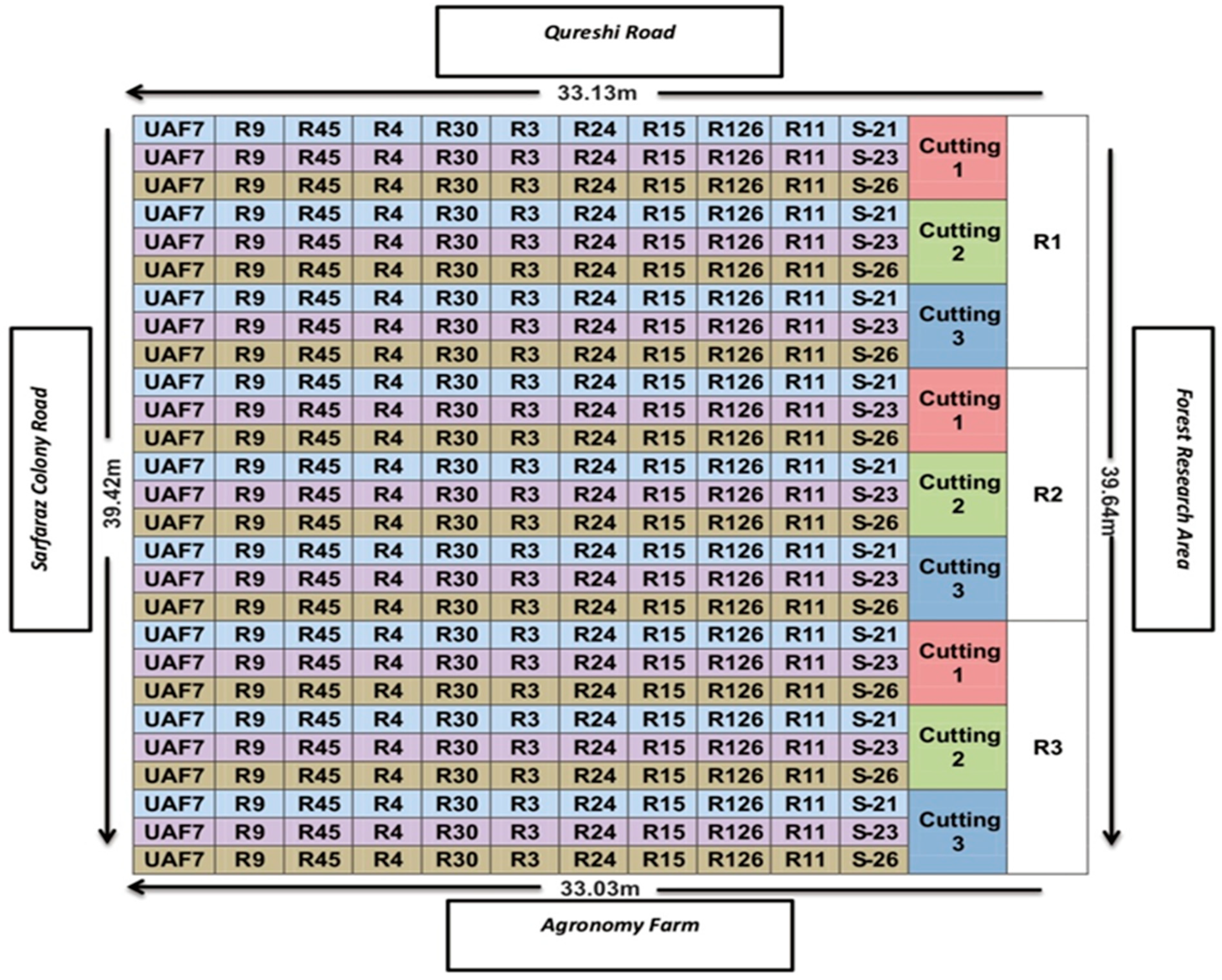
Figure 1. Split–split plot layout of the experimental site for two growing seasons. R1, R2, and R3 represent the three replicates; S-21, S-23, and S-26 represent three different spacing levels; and R11, R126, … and UAF7 are the ten studied quinoa accessions.
Sustainability 15 11446 g001
Figure 2. Illustration for different levels of cutting at different growth stages. Each plot was divided into three equal portions for each cutting. (Sustainability 15 11446 i001 ) represent plant residues after harvesting. Note: For leaves’ quality traits, the prefix “L” was used with each trait, in other words, LCP, LCF, LADF, and LNDF. Similarly, for stems, the prefix “S” was used with each trait, in other words, SCP, SCF, SADF and SNDF.
Sustainability 15 11446 g002
Figure 3. Climograph of the experimental site based on the air temperature (T_min and T_max), rainfall (mm), and humidity (%) distribution during the two experimental years (four months/year). (A) represents the climatic conditions of the first growing season (year 2018–2019) i.e., from November to February while (B) represents the climatic conditions of the second growing season (year 2019–2020) i.e., from November to February.
Sustainability 15 11446 g003
Figure 4. Cutting × spacing interaction ranking based on the MGIDI: (a) the selected combination (highlighted in red) based on their index value, considering 20% selection intensity (red line); (b) PCA plot shows the distribution of the studied traits and treatments; (c) selection differentials (%) for morphological, stem, and leaf quality traits were obtained from the selected interactions. Facets grouped the traits based on desired SDs.
Sustainability 15 11446 g004
Figure 5. The MGIDI ranks genotypes in descending order. (a) The non-selected and selected genotypes are shown in gray and red circles, respectively, and depending on the intensity (10%), the red circle depicts the cut point. (b) The proportion of every factor on the computed MGIDI represents the strengths and weaknesses of the selected genotypes. The smaller the ratio defined by a factor (near the outer edge), the closer the traits within that factor are to the ideotype. Dashed line represents the theoretical value if all the factors contributed equally. (c) Principal component analysis (PCA) biplot performed with the studied traits for the substrate factor. (d) Selection differentials (%) for morphological and stem and leaf quality traits were obtained from the selected genotypes. The traits are grouped by facets according to the desired selection differentials.
Sustainability 15 11446 g005
Figure 6. Comparison of leaf and stem qualities of selected quinoa genotypes with oat varieties being used as standard for forage. Oat data were recorded at the grain-filling stage, while quinoa genotype data at both cutting levels (C2 and C3; S: Spacing) were utilized for comparing the outcomes. (A) Leaf quality parameters: LCP: Leaf crude protein; LCF: leaf crude fat; LADF: leaf acid detergent fiber; LNDF: leaf neutral detergent fiber; LMois: leaf moisture. (B) Stem quality parameters: SCP: Stem crude protein; SCF: stem crude fat; SADF: stem acid detergent fiber; SNDF: stem neutral detergent fiber; SMois: stem moisture. The bars represent the standard error of mean.
Sustainability 15 11446 g006aSustainability 15 11446 g006b
Table 1. Predicted selection differentials, goals, and trait distributions of factors for the studied cutting × spacing interaction.
FactorsTraitsSenseXoXsSDSD%Goal
FA1PHincrease59.3591.5532.2054.26100
FA1NoLincrease148.94230.6681.7154.86100
FA1LAincrease34.9639.674.7113.46100
FA1Brincrease25.8534.658.7934.00100
FA1IDincrease4.615.290.6814.64100
FA1FWincrease91.32150.0058.6764.24100
FA1DWincrease18.3231.6313.3172.62100
FA1LCPincrease17.9320.943.0116.80100
FA1LCFincrease4.705.040.347.13100
FA1LADFdecrease22.0424.622.5811.710
FA1LNDFdecrease29.2631.842.588.830
FA1LMoisincrease11.2112.891.6814.96100
FA1SCPincrease13.0313.320.292.19100
FA1SCFincrease4.414.770.368.11100
FA1SADFdecrease24.0225.641.626.730
FA1SNDFdecrease34.3136.722.417.020
FA1SMoisincrease12.4614.632.1717.42100
total increase28.8
total decrease8.57
Note: SD%: Selection differential percentage; Xs: selected value; Xo: original value; SD: selection differential; PH: plant height; LA: leaf area; NoL: number of leaves; Br: no. of branches per plant; ID: internodal distance; FW: fresh weight; DW: dry weight; LCP: leaf crude protein; LCF: leaf crude fat; LADF: leaf acid detergent fiber; LNDF: leaf neutral detergent fiber; LMois: leaf moisture; SCP: stem crude protein; SCF: stem crude fat; SADF: stem acid detergent fiber; SNDF: stem neutral detergent fiber; SMois: stem moisture.
Table 2. Predicted selection differentials, goals, and trait distributions of factors for the studied genotypes.
FactorsTraitsSenseXoXsSDSD%Goal
FA1LAIncrease34.9635.130.170.49100
FA1LADFDecrease22.0420.09−1.95−8.83100
FA1LNDFDecrease29.2627.91−1.35−4.60100
FA1SADFDecrease24.0223.55−0.48−1.98100
FA1SMoisIncrease12.4612.660.211.66100
FA2PHIncrease59.3568.068.7114.68100
FA2LCPIncrease17.9318.340.412.28100
FA2LCFIncrease4.704.700.000.04100
FA2SNDFDecrease34.3134.890.581.700
FA3NoLIncrease148.94169.3120.3713.68100
FA3BrIncrease25.8526.430.582.23100
FA3FWIncrease91.32105.8314.5015.88100
FA3DWIncrease18.3221.082.7515.02100
FA4LMoisIncrease11.2111.290.080.68100
FA4SCPIncrease13.0313.270.241.81100
FA5IDIncrease4.624.54−0.07−1.610
FA5SCFIncrease4.414.510.102.16100
Total Increase5.31
Total Decrease−3.43
Note: SD%: Selection differential percentage; Xs: selected value; Xo: original value; SD: selection differential; PH: plant height; LA: leaf area; NoL: number of leaves; Br: no. of branches per plant; ID: internodal distance; FW: fresh weight; DW: dry weight; LCP: leaf crude protein; LCF: leaf crude fat; LADF: leaf acid detergent fiber; LNDF: leaf neutral detergent fiber; LMois: leaf moisture; SCP: stem crude protein; SCF: stem crude fat; SADF: stem acid detergent fiber; SNDF: stem neutral detergent fiber; SMois: stem moisture.
Disclaimer/Publisher’s Note: The statements, opinions and data contained in all publications are solely those of the individual author(s) and contributor(s) and not of MDPI and/or the editor(s). MDPI and/or the editor(s) disclaim responsibility for any injury to people or property resulting from any ideas, methods, instructions or products referred to in the content.