

An HBIM Integrated Approach Using Non-Destructive Techniques (NDT) to Support Energy and Environmental Improvement of Built Heritage: The Case Study of Palazzo Maffei Borghese in Rome

 ,
,  ,
,  ,
,  and
and 
Abstract
1. Introduction
1.1. Energy and Environmental Improvement of Built Heritage
1.2. The Role of Non-Destructive Techniques
1.3. The Role of Heritage Building Information Modelling
1.4. Research Aim
1.5. Research Gap and Noverlty
- lack of consolidated data on the characterisation of historical buildings;
- lack of a consolidated interdisciplinary process of data collection on historical buildings;
- lack of field application studies on the topic describing in detail the limitations, challenges and solutions proposed;
- need to tailor existing analysis and design methodologies and tools to historical buildings’ specificities and complexities.
2. Case Study Description
3. Methods
3.1. Description of the General Approach and the Specific Analyses Workflow
- ○
- studying rooms with the most common construction systems that emerged in the integrated analysis;
- ○
- analysing at least one room used continuously and one occasionally (to have a description of the most common types of uses, with also a different density of occupants in the room);
- ○
- monitoring the intermediate floors and understanding the behaviour of the building in portions that are less influenced by external forcings;
- ○
- covering as many exposures as possible;
- ○
- monitoring the office reception on the ground floor, as it is a very thermally dispersive space with discomfort issues, and the full-height internal gallery of Part-01 (Figure 4);
- ○
- studying the synergies between two “connected” rooms, one above the other.
3.2. IR Thermography Method
3.3. HFM Method
4. Experimental Set-Up
4.1. Measurement Equipment
4.2. Sensor Positioning
5. Results and Discussion
5.1. IR Thermography
- thermal bridges’ form and structure;
- different construction materials;
- discontinuities.
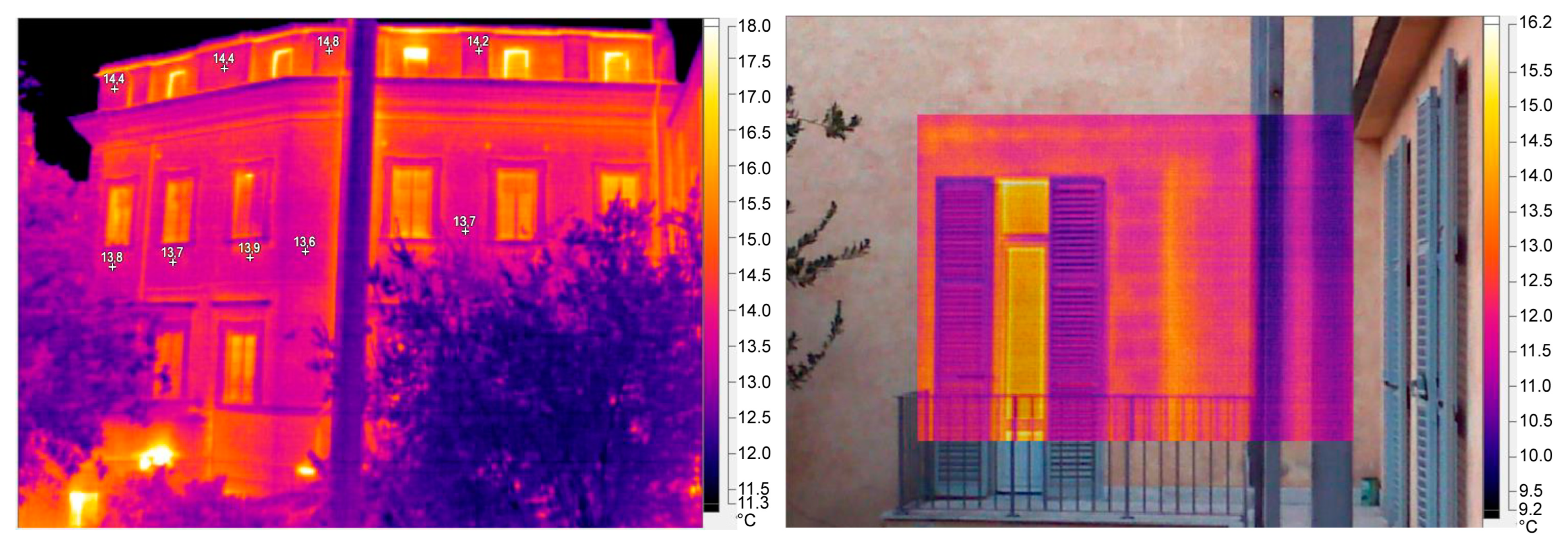
- The thermogram is processed by setting the background temperature to the value of the sky (−30 °C in the absence of clouds). Temperature markers are placed on part of the façade (upper part). Figure 14a shows the measurement point;
- The thermogram is post-processed by setting the reflected temperature to the value of the outdoor air temperature. Temperature markers are placed on part of the façade (lower part). Figure 14b shows the measurement point;
- Figure 15 shows that, in the upper part of the façade, the mark indicates the temperature of the surface, which has been compensated with the value of the reflected temperature of the sky. In the lower part of the façade, the mark indicates the surface temperature, with the value of the background temperature set to the value of the ambient temperature. The colour palette on the right side of the images refers to a background temperature with the value of the ambient temperature. For this reason, in cases where the viewing angle becomes larger, to capture the upper parts of the façades (for which compensation with the temperature of the sky is required), the temperature markings of the upper part of the façade do not correspond to the colour scheme of the image.
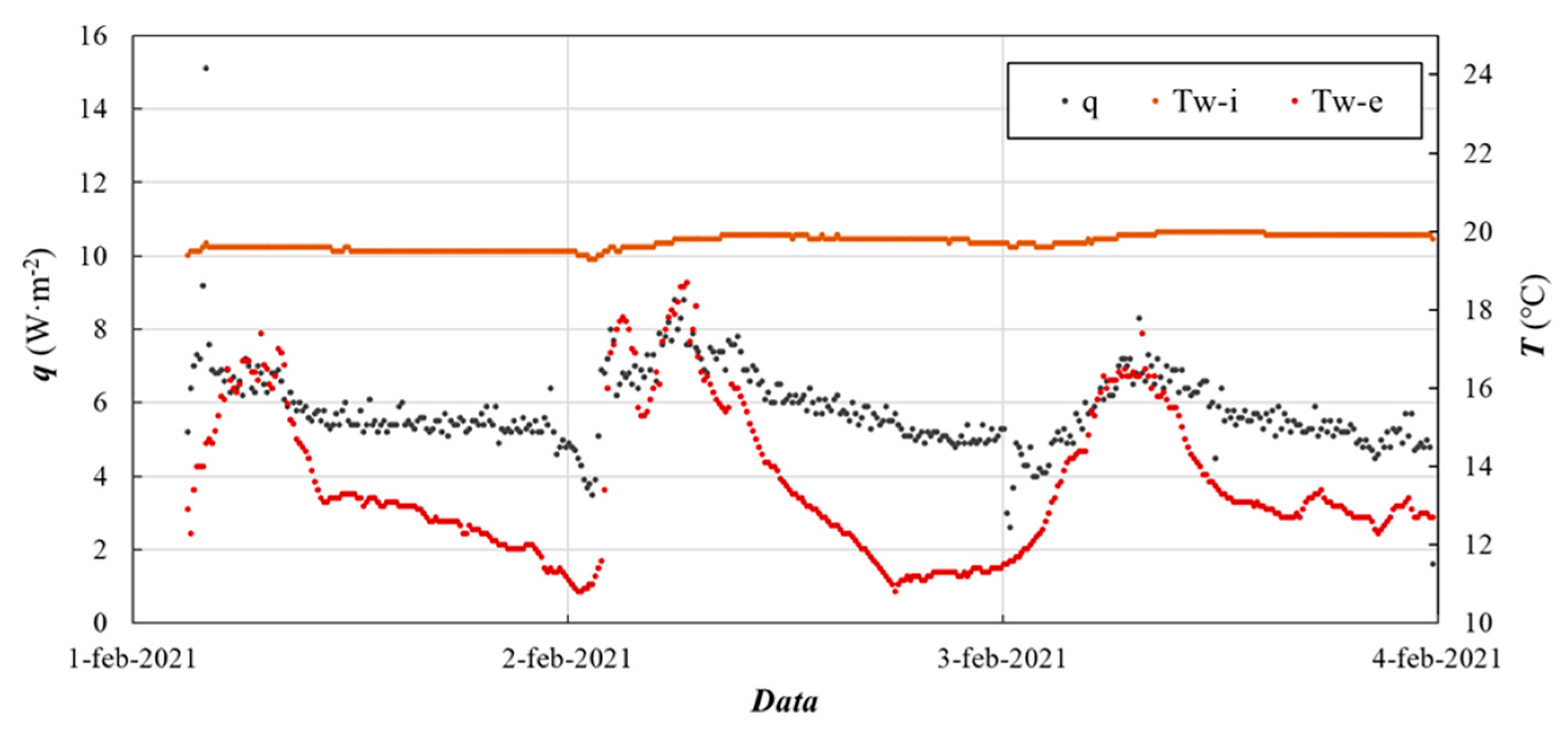
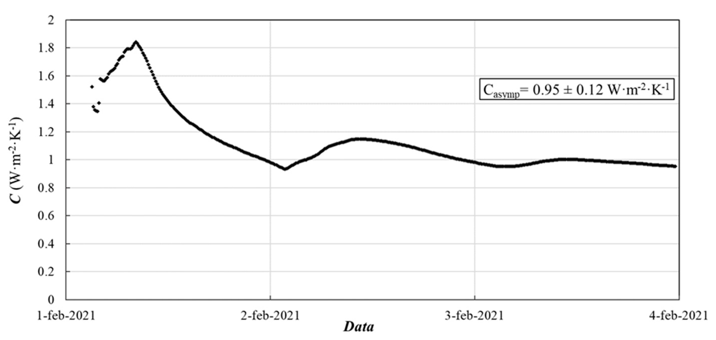
5.2. HFM
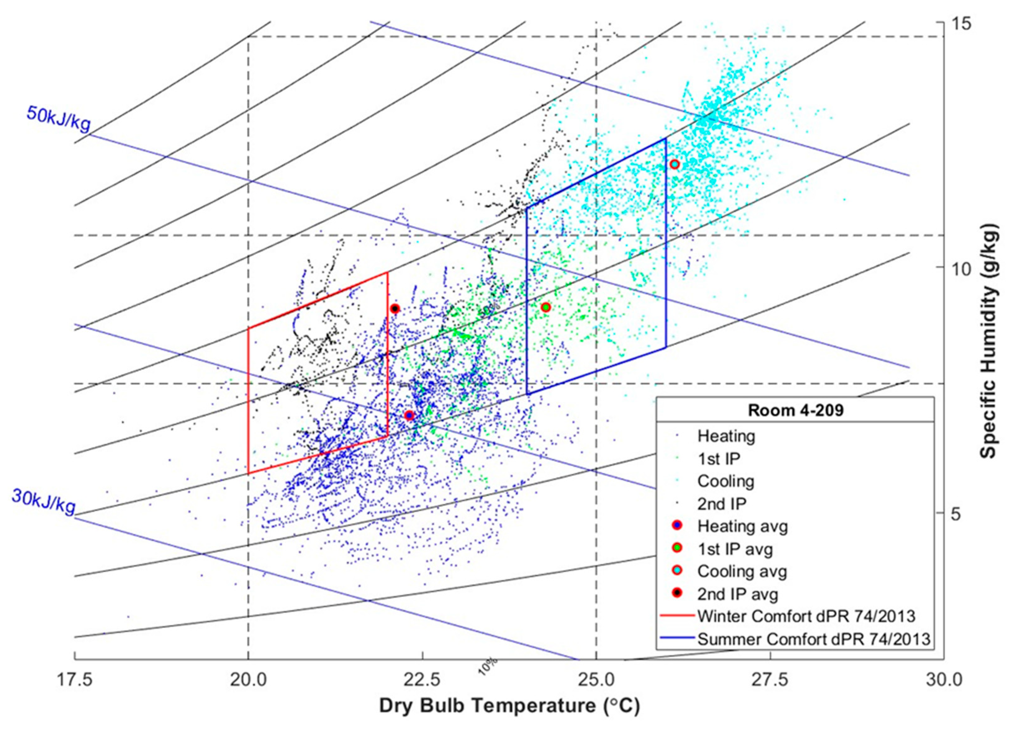
5.3. Microclimate Monitoring
- “Heating” from the 1 January to the 15 April and from the 1 November to the 31 December;
- “1st IP” (First Intermediate Period) from the 16 April to the 20 June;
- “Cooling” from the 21 June the 26 September;
- “2nd IP” (Second Intermediate Period) from the 27 September to the 30 October.
5.4. HBIM Integration
6. Conclusions
- ○
- the relevance of the careful planning of in situ activities and of preliminary supporting simulations to optimise time and cost, in synergy with the actors of the process;
- ○
- the crucial value of experts from all the different disciplines working together, both in the survey and measurement phase, as well as in the data elaboration phase, to achieve better results.
Author Contributions
Funding
Institutional Review Board Statement
Informed Consent Statement
Data Availability Statement
Acknowledgments
Conflicts of Interest
Nomenclature
| Latin | ||
| A | surface | [m2] |
| cp | specific heat | [J·kg−1·K−1] |
| C | conductance | [W·m−2·K−1] |
| heat flux for unit area | [W·m−2] | |
| thermal radiation power | [W] | |
| T | temperature | [K or °C] |
| U | heat transfer coefficient | W·m−2·K−1] |
| Greek | ||
| λ | thermal conductivity | W·m−1·K−1] |
| ε | emissivity | |
| ρ | density | [kg·m−3] |
| σ | Stefan–Boltzmann constant | W·m−2·K−4] |
| Subscripts | ||
| calc | calculated | |
| e | external | |
| i | internal | |
| meas | measured | |
| r | reflected | |
| w | wall | |
| Abbreviation | ||
| BIM | Building Information Modelling | |
| BPS | Building Performance Simulation | |
| CDE | Common Data Environment | |
| CDT | Cooling Day Type | |
| GHI | Global Horizontal Irradiance | |
| HBIM | Heritage Building Information Modelling | |
| HDT | Heating Day Type | |
| HFM | Heat Flow Meter | |
| HVAC | Heating Ventilation Air Conditioning | |
| IP | Intermediate Period | |
| IRT | Infrared Thermography | |
| NDT | Non-Destructive Techniques | |
| NWD | Non-Working Days | |
| RH | Relative Humidity | |
| WD | Working Days |
References
- Eurostat, Census Hub HC53. 2011. Available online: https://ec.europa.eu/CensusHub2/query.do?step=selectHyperCube&qhc=false (accessed on 13 January 2023).
- European Commission. Proposal for a Directive of The European Parliament and of the Council on the Energy Performance of Buildings (Recast). 2021. Available online: https://eur-lex.europa.eu/legal-content/EN/TXT/?uri=CELEX%3A52021PC0802&qid=1641802763889 (accessed on 9 September 2022).
- European Commission. Energy Performance of Buildings Directive. 2018. Available online: https://energy.ec.europa.eu/topics/energy-efficiency/energy-efficient-buildings/energy-performance-buildings-directive_en (accessed on 13 January 2023).
- Staniaszek, D. (Ed.) A Guide to Developing Strategies for Building Energy Renovation; BPIE: Brussels, Belgium, 2013. [Google Scholar]
- Economidou, M. (Ed.) Europe’s Buildings under the Microscope; Buildings Performance Institute Europe: Brussels, Belgium, 2011. [Google Scholar]
- European Commission. EU Buildings Factsheets. 2014. Available online: https://ec.europa.eu/energy/eu-buildings-factsheets_en (accessed on 9 September 2022).
- European Parliament. Directive (EU) 2018/844 of the European Parliament and of the Council of 30 May 2018 Amending Directive 2010/31/EU on the Energy Performance of Buildings and Directive 2012/27/EU on Energy Efficiency (Text with EEA Relevance). 2018. Available online: http://data.europa.eu/eli/dir/2018/844/oj/eng (accessed on 9 September 2022).
- European Parliament. Directive 2010/31/EU of the European Parliament and of the Council of 19 May 2010 on the Energy Performance of Buildings (Recast). 2010. Available online: http://data.europa.eu/eli/dir/2010/31/oj/eng (accessed on 9 September 2022).
- European Parliament. Directive 2012/27/EU of the European Parliament and of the Council of 25 October 2012 on Energy Efficiency, Amending Directives 2009/125/EC and 2010/30/EU and Repealing Directives 2004/8/EC and 2006/32/EC Text with EEA Relevance. 2012. Available online: http://data.europa.eu/eli/dir/2012/27/oj/eng (accessed on 9 September 2022).
- SECHURBA Project. Sustainable Energy Communities in Historic Urban Areas. 2008. Available online: https://ec.europa.eu/energy/intelligent/projects/sites/iee-projects/files/projects/documents/sechurba_guide_en.pdf (accessed on 9 September 2022).
- Gigliarelli, E.; Calcerano, F.; Cessari, L. Analytic Hierarchy Process. A Multi-Criteria Decision Support Approach for the Improvement of the Energy Efficiency of Built Heritage. In Proceedings of the EEHB2018 The 3rd International Confernece on Energy Efficiency in Historic Buildings, Tor Broström Lisa Nilsen Susanna Carlsten, Uppsala University, Department of Art History, Visby, Sweden, 26–28 September 2018; Available online: http://www.iea-shc.org/Data/Sites/1/publications/Energy-efficiency-in-historic-buildings_preliminary-conference-report.pdf (accessed on 9 September 2022).
- JPICH. Strategic Research Agenda—JPI Cultural Heritage and Global Change. 2014. Available online: http://www.jpi-culturalheritage.eu/wp-content/uploads/SRA-2014-06.pdf (accessed on 9 September 2022).
- JPICH. Strategic Research and Innovation Agenda 2020: Final Version of the Updated JPI CH SRIA Published. 2020. Available online: https://www.heritageresearch-hub.eu/strategic-research-and-innovation-agenda-2020-sria/ (accessed on 8 October 2021).
- Ballard, C.; Baron, N.; Bourgès, A.; Bucher, B.; Cassar, M.; Daire, M.-Y.; Daly, C.; Egusquiza, A.; Fatoric, S.; Holtorf, C.; et al. Cultural Heritage and Climate Change: New Challenges and Perspectives for Research. 2022. Available online: https://www.heritageresearch-hub.eu/white-paper-cultural-heritage-and-climate-change-new-challenges-and-perspectives-for-research/ (accessed on 5 April 2022).
- Troi, A.; Bastian, Z. Energy Efficiency Solutions for Historic Buildings a Handbook; Birkhäuser: Basel, Switzerland, 2015. [Google Scholar]
- Blumberga, A.; de Place, J.H. Ribuild: Written Guidelines for Decision Making Concerning the Possible Use of Internal Insulation in Historic Buildings. 2020. Available online: https://static1.squarespace.com/static/5e8c2889b5462512e400d1e2/t/5f04215c5b6cfa0aa7baa5b1/1594106230146/Written+guidelines+for+decision+making+concerning+the+possible.pdf (accessed on 9 September 2022).
- Kilian, R.; Leissner, J.; Antretter, F.; Holl, K.; Holm, A. Modeling Climate Change impact on Cultural Heritage—The European Project Climate for Culture. In Proceedings of the COST C26 Action Final Conference, Naples, Italy, 16–18 September 2010. [Google Scholar]
- Eriksson, P.; Hermann, C.; Hrabovszky-Horváth, S.; Rodwell, D. EFFESUS Methodology for Assessing the Impacts of Energy-Related Retrofit Measures on Heritage Significance, Hist. Environ. Policy Pract. 2014, 5, 132–149. [Google Scholar] [CrossRef]
- Andreotti, M.; Bottino-Leone, D.; Calzolari, M.; Davoli, P.; Pereira, L.D.; Lucchi, E.; Troi, A. Applied Research of the Hygrothermal Behaviour of an Internally Insulated Historic Wall without Vapour Barrier: In Situ Measurements and Dynamic Simulations. Energies 2020, 13, 3362. [Google Scholar] [CrossRef]
- Akkurt, G.G.; Aste, N.; Borderon, J.; Buda, A.; Calzolari, M.; Chung, D.; Costanzo, V.; Del Pero, C.; Evola, G.; Huerto-Cardenas, H.E.; et al. Dynamic thermal and hygrometric simulation of historical buildings: Critical factors and possible solutions, Renew. Sustain. Energy Rev. 2020, 118, 109509. [Google Scholar] [CrossRef]
- Heritage, E.W. Energy Heritage. A Guide to Improving Energy Efficiency in Traditional and Historic Homes. 2008. Available online: http://www.changeworks.org.uk/resources/energy-heritage-a-guide-to-improving-energy-efficiency-in-traditional-and-historic-homes (accessed on 9 September 2022).
- MIBACT, Linee Di Indirizzo Per Il Miglioramento Dell’efficienza Energetica Nel Patrimonio Culturale. Architettura, Centri e Nuclei Storici Ed Urbani. 2015. Available online: http://www.beap.beniculturali.it/opencms/multimedia/BASAE/documents/2015/10/27/1445954374955_Linee_indirizzo_miglioramento_efficienza_energetica_nel_patrimonio_culturale.pdf (accessed on 9 September 2022).
- Carbonara, G. Energy efficiency as a protection tool. Energy Build. 2015, 95, 9–12. [Google Scholar] [CrossRef]
- Gigliarelli, E.; Calcerano, F.; Cessari, L.; Bim, H. Numerical Simulation and Decision Support Systems: An Integrated Approach for Historical Buildings Retrofit. Energy Procedia 2017, 133, 135–144. [Google Scholar] [CrossRef]
- Potts, A. European Cultural Heritage Green Paper; Europa Nostra: Hague, The Netherlands, 2021. [Google Scholar]
- Cornaro, C.; Puggioni, V.A.; Strollo, R.M. Dynamic simulation and on-site measurements for energy retrofit of complex historic buildings: Villa Mondragone case study. J. Build. Eng. 2016, 6, 17–28. [Google Scholar] [CrossRef]
- Frasca, F.; Cornaro, C.; Siani, A.M. A method based on environmental monitoring and building dynamic simulation to assess indoor climate control strategies in the preventive conservation within historical buildings. Sci. Technol. Built Environ. 2019, 25, 1253–1268. [Google Scholar] [CrossRef]
- Frasca, F.; Verticchio, E.; Cornaro, C.; Siani, A.M. Performance assessment of hygrothermal modelling for diagnostics and conservation in an Italian historical church. Build. Environ 2021, 193, 107672. [Google Scholar] [CrossRef]
- Kilic, G. Using advanced NDT for historic buildings: Towards an integrated multidisciplinary health assessment strategy. J. Cult. Herit. 2015, 16, 526–535. [Google Scholar] [CrossRef]
- Tejedor, B.; Lucchi, E.; Bienvenido-Huertas, D.; Nardi, I. Non-destructive techniques (NDT) for the diagnosis of heritage buildings: Traditional procedures and futures perspectives. Energy Build. 2022, 263, 112029. [Google Scholar] [CrossRef]
- Lucchi, E. Applications of the infrared thermography in the energy audit of buildings: A review. Renew. Sustain. Energy Rev. 2018, 82, 3077–3090. [Google Scholar] [CrossRef]
- Dias, I.S.; Flores-Colen, I.; Silva, A. Critical Analysis about Emerging Technologies for Building’s Façade Inspection. Buildings 2021, 11, 53. [Google Scholar] [CrossRef]
- Kylili, A.; Fokaides, P.A.; Christou, P.; Kalogirou, S.A. Infrared thermography (IRT) applications for building diagnostics: A review. Appl. Energy. 2014, 134, 531–549. [Google Scholar] [CrossRef]
- Fox, M.; Goodhew, S.; De Wilde, P. Building defect detection: External versus internal thermography. Build. Environ. 2016, 105, 317–331. [Google Scholar] [CrossRef]
- Kirimtat, A.; Krejcar, O. A review of infrared thermography for the investigation of building envelopes: Advances and prospects. Energy Build. 2018, 176, 390–406. [Google Scholar] [CrossRef]
- Bisegna, F.; Ambrosini, D.; Paoletti, D.; Sfarra, S.; Gugliermetti, F. A qualitative method for combining thermal imprints to emerging weak points of ancient wall structures by passive infrared thermography—A case study. J. Cult. Herit. 2014, 15, 199–202. [Google Scholar] [CrossRef]
- Paoletti, D.; Ambrosini, D.; Sfarra, S.; Bisegna, F. Preventive thermographic diagnosis of historical buildings for consolidation. J. Cult. Herit. 2013, 14, 116–121. [Google Scholar] [CrossRef]
- Pescari, S.; Budău, L.; Vîlceanu, B. Rehabilitation and restauration of the main façade of historical masonry building –Romanian National Opera Timisoara. Case Stud. Constr. Mater. 2023, 18, e01838. [Google Scholar] [CrossRef]
- Kilic, G. Assessment of historic buildings after an earthquake using various advanced techniques. Structures 2023, 50, 538–560. [Google Scholar] [CrossRef]
- Cascardi, A.; Longo, F.; Perrone, D.; Lassandro, P.; Aiello, M.A. Thermography Investigation and Seismic Vulnerability Assessment of a Historical Vaulted Masonry Building. Heritage 2022, 5, 2041–2061. [Google Scholar] [CrossRef]
- Avdelidis, N.P.; Moropoulou, A. Applications of infrared thermography for the investigation of historic structures. J. Cult. Herit. 2004, 5, 119–127. [Google Scholar] [CrossRef]
- Valluzzi, M.R.; Lorenzoni, F.; Deiana, R.; Taffarel, S.; Modena, C. Non-destructive investigations for structural qualification of the Sarno Baths, Pompeii. J. Cult. Herit. 2019, 40, 280–287. [Google Scholar] [CrossRef]
- Meola, C. Infrared Thermography in the Architectural Field. Sci. World J. 2013, 2013, 323948. [Google Scholar] [CrossRef] [PubMed]
- Falchi, L.; Slanzi, D.; Balliana, E.; Driussi, G.; Zendri, E. Rising damp in historical buildings: A Venetian perspective. Build. Environ. 2018, 131, 117–127. [Google Scholar] [CrossRef]
- Barbosa, M.T.G.; Rosse, V.J.; Laurindo, N.G. Thermography evaluation strategy proposal due moisture damage on building facades. J. Build. Eng. 2021, 43, 102555. [Google Scholar] [CrossRef]
- Rosina, E.; Zala, M.; Ammendola, A. The moisture issue affecting the historical buildings in the Po valley: A case study approach. J. Cult. Herit. 2023, 60, 78–85. [Google Scholar] [CrossRef]
- Trevisiol, F.; Barbieri, E.; Bitelli, G. Multitemporal Thermal Imagery Acquisition and Data Processing on Historical Masonry: Experimental Application on a Case Study. Sustainability 2022, 14, 559. [Google Scholar] [CrossRef]
- Nardi, I.; de Rubeis, T.; Taddei, M.; Ambrosini, D.; Sfarra, S. The energy efficiency challenge for a historical building undergone to seismic and energy refurbishment. Energy Procedia 2017, 133, 231–242. [Google Scholar] [CrossRef]
- De Berardinis, P.; Bartolomucci, C.; Capannolo, L.; De Vita, M.; Laurini, E.; Marchionni, C. Instruments for Assessing Historical Built Environments in Emergency Contexts: Non-Destructive Techniques for Sustainable Recovery. Buildings 2018, 8, 27. [Google Scholar] [CrossRef]
- Bienvenido-Huertas, D.; Moyano, J.; Marín, D.; Fresco-Contreras, R. Review of in situ methods for assessing the thermal transmittance of walls. Renew. Sustain. Energy Rev. 2019, 102, 356–371. [Google Scholar] [CrossRef]
- Teni, M.; Krstić, H.; Kosiński, P. Review and comparison of current experimental approaches for in-situ measurements of building walls thermal transmittance. Energy Build. 2019, 203, 109417. [Google Scholar] [CrossRef]
- ISO 6946:2007; Building Components and Building Elements—Thermal Resistance and Thermal Transmittance—Calculation Method. 2007. Available online: https://www.iso.org/standard/40968.html (accessed on 9 September 2022).
- ISO 9869-1:2014; Thermal Insulation—Building Elements—In-Situ Measurement of Thermal Resistance and Thermal Transmittance—Part 1: Heat flow Meter Method. 2014. Available online: https://www.iso.org/standard/59697.html (accessed on 9 September 2022).
- Bienvenido-Huertas, D.; Rodríguez-Álvaro, R.; Moyano, J.J.; Rico, F.; Marín, D. Determining the U-Value of Façades Using the Thermometric Method: Potentials and Limitations. Energies 2018, 11, 360. [Google Scholar] [CrossRef]
- Fokaides, P.A.; Kalogirou, S.A. Application of infrared thermography for the determination of the overall heat transfer coefficient (U-Value) in building envelopes. Appl. Energy. 2011, 88, 4358–4365. [Google Scholar] [CrossRef]
- Dall’O’, G.; Sarto, L.; Panza, A. Infrared Screening of Residential Buildings for Energy Audit Purposes: Results of a Field Test. Energies 2013, 6, 3859–3878. [Google Scholar] [CrossRef]
- Albatici, R.; Tonelli, A.M. Infrared thermovision technique for the assessment of thermal transmittance value of opaque building elements on site. Energy Build. 2010, 42, 2177–2183. [Google Scholar] [CrossRef]
- Meng, X.; Gao, Y.; Wang, Y.; Yan, B.; Zhang, W.; Long, E. Feasibility experiment on the simple hot box-heat flow meter method and the optimization based on simulation reproduction. Appl. Therm. Eng. 2015, 83, 48–56. [Google Scholar] [CrossRef]
- Meng, X.; Luo, T.; Gao, Y.; Zhang, L.; Shen, Q.; Long, E. A new simple method to measure wall thermal transmittance in situ and its adaptability analysis. Appl. Therm. Eng. 2017, 122, 747–757. [Google Scholar] [CrossRef]
- Lucchi, E. Thermal transmittance of historical brick masonries: A comparison among standard data, analytical calculation procedures, and in situ heat flow meter measurements. Energy Build. 2017, 134, 171–184. [Google Scholar] [CrossRef]
- Lucchi, E. Thermal transmittance of historical stone masonries: A comparison among standard, calculated and measured data. Energy Build. 2017, 151, 393–405. [Google Scholar] [CrossRef]
- Tejedor, B.; Casals, M.; Gangolells, M.; Roca, X. Quantitative internal infrared thermography for determining in-situ thermal behaviour of façades. Energy Build. 2017, 151, 187–197. [Google Scholar] [CrossRef]
- Tejedor, B.; Barreira, E.; Almeida, R.M.S.F.; Casals, M. Automated data-processing technique: 2D Map for identifying the distribution of the U-value in building elements by quantitative internal thermography. Autom. Constr. 2021, 122, 103478. [Google Scholar] [CrossRef]
- Ascione, F.; Ceroni, F.; De Masi, R.F.; Rossi, F.D.; Pecce, M.R. Historical buildings: Multidisciplinary approach to structural/energy diagnosis and performance assessment. Appl. Energy. 2017, 185, 1517–1528. [Google Scholar] [CrossRef]
- Roque, E.; Vicente, R.; Almeida, R.M.S.F.; da Silva, J.M.; Ferreira, A.V. Thermal characterisation of traditional wall solution of built heritage using the simple hot box-heat flow meter method: In situ measurements and numerical simulation. Appl. Therm. Eng. 2020, 169, 114935. [Google Scholar] [CrossRef]
- Baker, P. U-Values and Traditional Buildings-In Situ Measurements and Their Comparisons to Calculated Values; Technical Paper 10; Glasgow Caledonian University: Glasgow, UK, 2010. [Google Scholar]
- De Berardinis, P.; Rotilio, M.; Marchionni, C.; Friedman, A. Improving the energy-efficiency of historic masonry buildings. A case study: A minor centre in the Abruzzo region, Italy. Energy Build. 2014, 80, 415–423. [Google Scholar] [CrossRef]
- Williamson, J.B.; Stinson, J.; Garnier, C.; Currie, J. In-Situ Monitoring of Thermal Refurbishment on Pre-1919 Properties in Scotland. Int. J. Sustain. Constr. 2014, 2, 26–33. [Google Scholar]
- Sassine, E.; Younsi, Z.; Cherif, Y.; Chauchois, A.; Antczak, E. Experimental determination of thermal properties of brick wall for existing construction in the north of France. J. Build. Eng. 2017, 14, 15–23. [Google Scholar] [CrossRef]
- Sassine, E.; Younsi, Z.; Cherif, Y.; Antczak, E. Thermal performance evaluation of a massive brick wall under real weather conditions via the Conduction Transfer function method. Case Stud. Constr. Mater. 2017, 7, 56–65. [Google Scholar] [CrossRef]
- Evangelisti, L.; Guattari, C.; Gori, P.; Asdrubali, F. Assessment of equivalent thermal properties of multilayer building walls coupling simulations and experimental measurements. Build. Environ. 2018, 127, 77–85. [Google Scholar] [CrossRef]
- Berger, J.; Kadoch, B. Estimation of the thermal properties of an historic building wall by combining modal identification method and optimal experiment design. Build. Environ. 2020, 185, 107065. [Google Scholar] [CrossRef]
- Sassine, E.; Cherif, Y.; Antczak, E. Parametric identification of thermophysical properties in masonry walls of buildings. J. Build. Eng. 2019, 25, 100801. [Google Scholar] [CrossRef]
- Hatır, M.E.; İnce, İ.; Bozkurt, F. Investigation of the effect of microclimatic environment in historical buildings via infrared thermography. J. Build. Eng. 2022, 57, 104916. [Google Scholar] [CrossRef]
- Cruz, C.; Gaju, M.; Gallego, A.; Rescalvo, F.; Suarez, E. Non-Destructive Multi-Feature Analysis of a Historic Wooden Floor. Buildings 2022, 12, 2193. [Google Scholar] [CrossRef]
- Martorana, R.; Capizzi, P. Joint Investigation with Ground Penetrating Radar and Infrared Thermography as a Diagnostic Support for the Restoration of Two Wall Mosaics in the Church of St. Mary of the Admiral in Palermo, Italy. Heritage 2022, 5, 2298–2314. [Google Scholar] [CrossRef]
- Coli, M.; Ciuffreda, A.L.; Marchetti, E.; Morandi, D.; Luceretti, G.; Lippi, Z. 3D HBIM Model and Full Contactless GPR Tomography: An Experimental Application on the Historic Walls That Support Giotto’s Mural Paintings, Santa Croce Basilica, Florence—Italy. Heritage 2022, 5, 2534–2546. [Google Scholar] [CrossRef]
- Providakis, C.P.; Mousteraki, M.G.; Providaki, G.C. Operational Modal Analysis of Historical Buildings and Finite Element Model Updating Using α Laser Scanning Vibrometer. Infrastructures 2023, 8, 37. [Google Scholar] [CrossRef]
- Piroddi, L.; Rassu, M. Application of GPR Prospection to Unveil Historical Stratification inside Monumental Buildings: The Case of San Leonardo de Siete Fuentes in Santu Lussurgiu, Sardinia, Italy. Land 2023, 12, 590. [Google Scholar] [CrossRef]
- Santini, S.; Borghese, V.; Baggio, C. HBIM-Based Decision-Making Approach for Sustainable Diagnosis and Conservation of Historical Timber Structures. Sustainability 2023, 15, 3. [Google Scholar] [CrossRef]
- Santini, S.; Cogotti, M.; Baggio, C.; Sabbatini, V.; Sebastiani, C. Field testing for structural behavior of a stratified monumental complex over time: Palazzo Colonna-Barberini and Templum Fortunae Praeneste. Case Stud. Constr. Mater. 2023, 18, e02152. [Google Scholar] [CrossRef]
- de Santoli, L. Guidelines on energy efficiency of cultural heritage. Energy Build. 2015, 86, 534–540. [Google Scholar] [CrossRef]
- Delegou, E.T.; Mourgi, G.; Tsilimantou, E.; Ioannidis, C.; Moropoulou, A. A Multidisciplinary Approach for Historic Buildings Diagnosis: The Case Study of the Kaisariani Monastery. Heritage 2019, 2, 1211–1232. [Google Scholar] [CrossRef]
- Bruno, S.; De Fino, M.; Fatiguso, F. Historic Building Information Modelling: Performance assessment for diagnosis-aided information modelling and management. Autom. Constr. 2018, 86, 256–276. [Google Scholar] [CrossRef]
- Calcerano, F.; Thravalou, S.; Martinelli, L.; Alexandrou, K.; Artopoulos, G.; Gigliarelli, E. Energy and environmental improvement of built heritage: HBIM simulation-based approach applied to nine Mediterranean case-studies. Build. Res. Inf. 2023, 1–23. [Google Scholar] [CrossRef]
- Gigliarelli, E.; Calcerano, F.; D’Uffizi, F.; Di Biccari, C.; Mangialardi, G.; Campari, M. From Heritage BIM to BPS, a computational design-based interoperability approach. In Proceedings of the 16th IBPSA Conference, Rome, Italy, 2–4 September 2019. [Google Scholar]
- ISO 19650:2018; Organization and Digitization of Information about Buildings and Civil Engineering Works, Including Building Information Modelling (BIM)—Information Management Using Building Information Modelling. ISO: Geneva, Switzerland, 2018.
- National BIM Standard Building. SMART alliance. Part 1: Overview, Principles, and methodologies. In National Building Information Modeling Standard; Harris, D., Ed.; National Institute of Building Sciences: Washington, DC, USA, 2007. [Google Scholar]
- Eastman, C.M.; Teicholz, P.M.; Sacks, R.; Lee, G. BIM Handbook: A Guide to Building Information Modeling for Owners, Managers, Designers, Engineers and Contractors, 3rd ed.; Wiley: Hoboken, NJ, USA, 2018. [Google Scholar]
- Pocobelli, D.P.; Boehm, J.; Bryan, P.; Still, J.; Grau-Bové, J. BIM for heritage science: A review. Herit. Sci. 2018, 6, 30. [Google Scholar] [CrossRef]
- Bruno, N.; Roncella, R. HBIM for Conservation: A New Proposal for Information Modeling. Remote Sens. 2019, 11, 1751. [Google Scholar] [CrossRef]
- Mora, R.; Sánchez-Aparicio, L.J.; Maté-González, M.Á.; García-Álvarez, J.; Sánchez-Aparicio, M.; González-Aguilera, D. An historical building information modelling approach for the preventive conservation of historical constructions: Application to the Historical Library of Salamanca. Autom. Constr. 2021, 121, 103449. [Google Scholar] [CrossRef]
- Jouan, P.; Hallot, P. Digital Twin: Research Framework to Support Preventive Conservation Policies. ISPRS Int. J. Geo-Inf. 2020, 9, 228. [Google Scholar] [CrossRef]
- Di Giuda, G.M.; Giana, P.E.; Schievano, M.; Paleari, F. Guidelines to Integrate BIM for Asset and Facility Management of a Public University. In Digital Transformation of the Design, Construction and Management Processes of the Built Environment; Springer: Berlin/Heidelberg, Germany, 2020; pp. 309–318. [Google Scholar] [CrossRef]
- Bastem, S.S.; Cekmis, A. Development of historic building information modelling: A systematic literature review. Build. Res. Inf. 2022, 50, 527–558. [Google Scholar] [CrossRef]
- Moyano, J.; Carreño, E.; Nieto-Julián, J.E.; Gil-Arizón, I.; Bruno, S. Systematic approach to generate Historical Building Information Modelling (HBIM) in architectural restoration project. Autom. Constr. 2022, 143, 104551. [Google Scholar] [CrossRef]
- Cursi, S.; Martinelli, L.; Paraciani, N.; Calcerano, F.; Gigliarelli, E. Linking external knowledge to heritage BIM. Autom. Constr. 2022, 141, 104444. [Google Scholar] [CrossRef]
- Chiabrando, F.; Donato, V.; Turco, M.L.; Santagati, C. Cultural Heritage Documentation, Analysis and Management Using Building Information Modelling: State of the Art and Perspectives. In Mechatronics for Cultural Heritage and Civil Engineering; Springer: Berlin/Heidelberg, Germany, 2018; pp. 181–202. [Google Scholar] [CrossRef]
- Bruno, S.; Musicco, A.; Fatiguso, F.; Dell’Osso, G.R. The Role of 4D Historic Building Information Modelling and Management in the Analysis of Constructive Evolution and Decay Condition within the Refurbishment Process. Int. J. Archit. Herit. 2021, 15, 1250–1266. [Google Scholar] [CrossRef]
- Angulo-Fornos, R.; Castellano-Román, M. HBIM as Support of Preventive Conservation Actions in Heritage Architecture. Experience of the Renaissance Quadrant Façade of the Cathedral of Seville. Appl. Sci. 2020, 10, 2428. [Google Scholar] [CrossRef]
- Santagati, C.; Papacharalambous, D.; Sanfilippo, G.; Bakirtzis, N.; Laurini, C.; Hermon, S. HBIM approach for the knowledge and documentation of the St. John the Theologian cathedral in Nicosia (Cyprus). J. Archaeol. Sci. Rep. 2021, 36, 102804. [Google Scholar] [CrossRef]
- Mammoli, R.; Mariotti, C.; Quattrini, R. Modeling the Fourth Dimension of Architectural Heritage: Enabling Processes for a Sustainable Conservation. Sustainability 2021, 13, 5173. [Google Scholar] [CrossRef]
- Simeone, D.; Cursi, S.; Acierno, M. BIM semantic-enrichment for built heritage representation. Autom. Constr. 2019, 97, 122–137. [Google Scholar] [CrossRef]
- Quattrini, R.; Pierdicca, R.; Morbidoni, C. Knowledge-based data enrichment for HBIM: Exploring high-quality models using the semantic-web. J. Cult. Herit. 2017, 28, 129–139. [Google Scholar] [CrossRef]
- Barontini, A.; Alarcon, C.; Sousa, H.S.; Oliveira, D.V.; Masciotta, M.G.; Azenha, M. Development and Demonstration of an HBIM Framework for the Preventive Conservation of Cultural Heritage. Int. J. Archit. Herit. 2022, 16, 1451–1473. [Google Scholar] [CrossRef]
- Vieira, M.; Ribeiro, G.; Alves, K.; Barbosa, J.E.; Isidoro, H.; Martins, T.; Magalhães, B.K.; Almeida, F.E.; Moreira, E.; Mesquita, E. Updating the documentation of a historic building: A case study of the José de Alencar theatre. J. Build. Pathol. Rehabil. 2023, 8, 36. [Google Scholar] [CrossRef]
- Antonopoulou, S.; Bryan, P. BIM for Heritage: Developing a Historic Building Information Model; Historic England: Swindon, UK, 2017. [Google Scholar]
- Palomar, I.J.; Valldecabres, J.L.G.; Tzortzopoulos, P.; Pellicer, E. An online platform to unify and synchronise heritage architecture information. Autom. Constr. 2020, 110, 103008. [Google Scholar] [CrossRef]
- Spiridigliozzi, G.; Pompei, L.; Cornaro, C.; Santoli, L.D.; Bisegna, F. BIM-BEM support tools for early stages of zero-energy building design. IOP Conf. Ser. Mater. Sci. Eng. 2019, 609, 072075. [Google Scholar] [CrossRef]
- Spiridigliozzi, G.; De Santoli, L.; Cornaro, C.; Basso, G.L.; Barati, S. BIM tools interoperability for designing energy-efficient buildings. AIP Conf. Proc. 2019, 2191, 020140. [Google Scholar] [CrossRef]
- Pompei, L.; Spiridigliozzi, G.; de Santoli, L.; Cornaro, C.; Bisegna, F. Testing the BIM-ladybug tools interoperability: A daylighting simulation workflow. Build. Simul. Appl. 2020, 149–156. Available online: https://www.scopus.com/inward/record.uri?eid=2-s2.0-85090829291&partnerID=40&md5=88ed552c80c27ef0276f99235a5f1984 (accessed on 9 September 2022).
- Gigliarelli, E.; Calcerano, F.; Calvano, M.; Ruperto, F.; Sacco, M.; Cessari, L. Integrated numerical analysis and Building Information Modeling for Cultural Heritage. In Proceedings of the Conference: Building Simulation Application 2017, Bolzano, Italy, 8–11 February 2017. [Google Scholar]
- Nieto-Julián, J.E.; Lara, L.; Moyano, J. Implementation of a TeamWork-HBIM for the Management and Sustainability of Architectural Heritage. Sustainability 2021, 13, 2161. [Google Scholar] [CrossRef]
- Piselli, C.; Romanelli, J.; Di Grazia, M.; Gavagni, A.; Moretti, E.; Nicolini, A.; Cotana, F.; Strangis, F.; Witte, H.J.L.; Pisello, A.L. An Integrated HBIM Simulation Approach for Energy Retrofit of Historical Buildings Implemented in a Case Study of a Medieval Fortress in Italy. Energies 2020, 13, 2601. [Google Scholar] [CrossRef]
- Khodeir, L.M.; Aly, D.; Tarek, S. Integrating HBIM (Heritage Building Information Modeling) Tools in the Application of Sustainable Retrofitting of Heritage Buildings in Egypt. Procedia Environ. Sci. 2016, 34, 258–270. [Google Scholar] [CrossRef]
- Al-Sakkaf, A.; Bagchi, A.; Zayed, T.; Mahmoud, S. Sustainability assessment model for heritage buildings. Smart Sustain. Built Environ. 2023, 12, 105–127. [Google Scholar] [CrossRef]
- Gigliarelli, E.; Calcerano, F.; Martinelli, L.; Cessari, L. A Methodology for Built Heritage Energy and Environmental Improvement: The BEEP Project. In Proceedings of the Heritage for the Future, Science for Heritage, Paris, France, 15–16 March 2022. [Google Scholar]
- Croci, G. General methodology for the structural restoration of historic buildings: The cases of the Tower of Pisa and the Basilica of Assisi. J. Cult. Herit. 2000, 1, 7–18. [Google Scholar] [CrossRef]
- Aurigemma, M.G. Palazzo Firenze in Campo Marzio; Istituto Poligrafico e Zecca dello Stato, Libreria dello Stato: Foggia, Italy, 2007. [Google Scholar]
- Aurigemma, M.G. Introduzione a Palazzo Firenze; Società Dante Alighieri, Edilazio: Rome, Italy, 2012. [Google Scholar]
- Giovannetti, F. Manuale del Recupero del Comune di Roma; DEI: Rome, Italy, 2004. [Google Scholar]
- Formenti, C.; Cortelletti, A. La Pratica del Fabbricare; Hoepli: Milan, Italy, 1933. [Google Scholar]
- Holman, J.P. Heat Transfer: Tenth Edition; McGraw-Hill Education: New York, NY, USA, 2010. [Google Scholar]
- Vollmer, M. Infrared Thermal Imaging. In Computer Vision; Ikeuchi, K., Ed.; Springer International Publishing: Cham, The Switzerland, 2021; pp. 666–670. [Google Scholar] [CrossRef]
- Tubi, N.; Silva, M.P.; Ditri, F. Gli Edifici in Pietra—Recupero e Costruzione—Murature, Solai—Analisi Bioclimatica e Ambientale; Sistemi Editoriali: Napoli Italy, 2009. [Google Scholar]
- Corrado, V.; Ballarini, I.; Corgnati, S.P. Typology Approach for Building Stock Energy Assessment; TABULA Project Team: Torino, Italy, 2012. [Google Scholar]
- UNI/TR 11552:2014; Abaco Delle Strutture Costituenti L’involucro Opaco Degli Edifici—Parametri Termofisici. 2014. Available online: https://store.uni.com/uni-tr-11552-2014 (accessed on 9 September 2022).
- UNI 10351:2021; Materiali da Costruzione—Proprietà Termoigrometriche—Procedura per La Scelta Dei Valori Di Progetto. 2021. Available online: https://store.uni.com/uni-10351-2021 (accessed on 9 September 2022).
- UNI EN ISO 6946:2018; Componenti ed Elementi per Edilizia—Resistenza Termica e Trasmittanza Termica—Metodi di Calcolo. 2018. Available online: https://store.uni.com/uni-en-iso-6946-2018 (accessed on 9 September 2022).
- D.P.R. 74, Decreto del Presidente della Repubblica 16 aprile 2013, n. 74. Regolamento Recante Definizione dei Criteri Generali in Materia di Esercizio, Conduzione, Controllo, Manutenzione e Ispezione Degli Impianti Termici per la Climatizzazione Invernale ed Estiva degli Edifici e per la preparazione dell’Acqua Calda per usi Igienici Sanitari, a Norma dell’Articolo 4, Comma 1, Lettere a) e c), del d.lgs. 19 Agosto 2005, n. 192 (G.U. n. 149 del 27 Giugno 2013). 2013. Available online: https://www.gazzettaufficiale.it/eli/id/20136/27/13G00114/sg (accessed on 9 September 2022).
- Gigliarelli, E.; Calcerano, F.; Martinelli, L.; Artopoulos, G.; Thravalou, S.; Alexandrou, K. Methodology for the Energy Renovation of Heritage Buildings Using BIM.; CNR Edizioni: Rome, Italy, 2022. [Google Scholar]


| Main Specifications | |
|---|---|
| Detector type | Focal plane array uncooled microbolometer |
| Resolution | 320 × 240 pixels |
| Noise Equivalent Temperature Difference (NETD) | ≤0.045 °C (45 mK) |
| Infrared spectral band | 7.5–14 μm (long wave) |
| Minimum focus distance | 46 cm |
| Temperature measurements range | −20 °C to 600 °C |
| Temperature measurements accuracy | ±2 °C or 2% |
| Image capture frequency | 9 Hz |
| Lens Type | |
| Field of view | 23° × 17° |
| Spatial resolution (IFOV) | 1.25 mRad |
| Minimum focus distance | 15 cm |
| Producer | Model | Type | Temp. Range | Accuracy | |
|---|---|---|---|---|---|
| HFM | Ahlborn | Almeno FQA017C | 117 | −40–80 °C | 5% @ 25 °C |
| Thermocouples | Ahlborn | Almeno FTA3901L03 | NiCr-Ni | −25–400 °C | Class 2 (DIN/IEC 582/2) |
| Relative Humidity | Temperature | |
|---|---|---|
| Accuracy | ±2% | ±0.3 °C |
| Resolution | 0.01% | 0.015 °C |
| Measurement range | 0–100% | −40–125 °C |
| Response time | 8 s | >2 s |
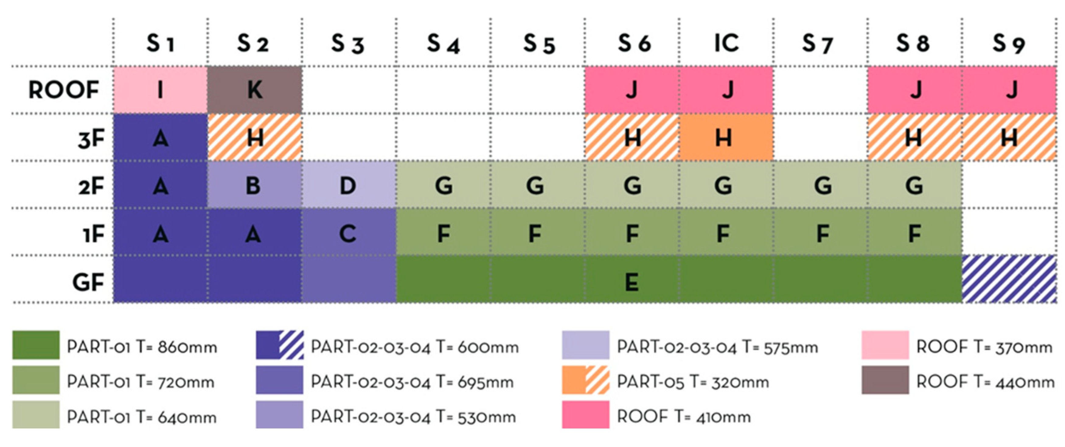
| Activity | Sensor # | Room Code | Floor | Exposure | Type of Masonry (Figure 6) |
|---|---|---|---|---|---|
| HFM | 1 | 220 | 2 | Northeast | D |
| HFM | 2 | 116 | 1 | Northeast | C |
| HFM | 3 | 127 | 1 | East | A |
| HFM | 4 | 234 | 2 | East | B |
| HFM | 5 | 105 | 1 | Northwest | F |
| HFM | 6 | 209 | 2 | Northwest | G |
| HFM | 7 | 318 | 3 | South, Internal Cloister | H |
| HFM | 8 | 318 | 3 | Roof | I |
| HFM | 9 | 344 | 3 | Roof | K |
| Activity | Sensor # | Room Code | Floor | Exposure, Use, and Density of Occupancy |
|---|---|---|---|---|
| Microclimate | 1 | 003 | G | Not applicable, office reception, low density of occupancy |
| Microclimate | 2 | 138 | 1 | Southeast, office, low density of occupancy |
| Microclimate | 3 | 208 | 2 | Not applicable, full-height internal gallery, service space |
| Microclimate | 4 | 209 | 2 | Northwest, office, low density of occupancy |
| Microclimate | 5 | 220 | 2 | Northeast, office, low density of occupancy |
| Microclimate | 6 | 247 | 2 | Southwest, office, high density of occupancy |
| Microclimate | 7 | 322 | 3 | Southwest, office, low density of occupancy |
| Microclimate | 8 | 344 | 3 | West, office, high density of occupancy |
| Orientation | Date (From–To) | Room # | Meas. # | C (W·m−2·K−1) | Ucalc (W·m−2·K−1) | Convergence |
|---|---|---|---|---|---|---|
| NORTH-EAST | 1 February 10:03–5 February 8:35 | 220 | 1 | 0.95 ± 0.12 | 0.82 | YES |
| NORTH-EAST | 5 February 10:59–9 February 8:39 | 116 | 2 | 0.81 ± 0.10 | 0.71 | NO |
| EAST | 9 February 10:45–16 February 8:40 | 127 | 3 | 0.56 ± 0.05 | 0.51 | YES |
| EAST | 16 February 11:02–23 February2 8:47 | 234 | 4 | 1.10 ± 0.11 | 0.92 | YES |
| NORTH-WEST | 23 February 10:43–26 February 7:53 | 105 | 5 | 0.62 ± 0.08 | 0.56 | YES |
| NORTH-WEST | 26 February 10:38–2 March 8:14 | 209 | 6 | 0.71 ± 0.07 | 0.63 | YES |
| SOUTH-Internal Cloister | 2 March 10:48–9 March 02:08 | 318 | 7 | 1.28 ± 0.14 | 1.05 | YES |
| ROOF | 10 March 11:19–11 March 14:19 | 318 | 8 | 1.06 ± 0.09 | 0.91 | YES |
| ROOF | 31 March 6:21–1 April 5:51 | 207 | 9 | 0.74 ± 0.07 | 0.66 | NO |
| Wall Package Simulation (IDA ICE) | Meas # | C (W·m−2·K−1) | Ucalc (W·m−2·K−1) | ||||||||
|---|---|---|---|---|---|---|---|---|---|---|---|
| Data | Room | Meas. | Sim. | MAE | NMAE (%) | Meas. | Sim. | MAE | NMAE (%) | ||
| East | 1 February 10:03–5 February 8:35 | 220 | 1 | 0.953 | 0.922 | 0.032 | 3.4 | 0.820 | 0.797 | 0.024 | 2.9 |
| 5 February 10:59–9 February 8:39 | 116 | 2 | 0.806 | 0.803 | 0.003 | 0.4 | 0.709 | 0.706 | 0.003 | 0.4 | |
| 9 February 10:45–16 February 8:40 | 127 | 3 | 0.560 | 0.630 | 0.071 | 11 | 0.511 | 0.569 | 0.058 | 10 | |
| 16 February 11:02–23 February 8:47 | 234 | 4 | 1.097 | 1.360 | 0.263 | 19 | 0.925 | 1.105 | 0.180 | 16 | |
| North | 23 February 10:43–26 February 7:53 | 105 | 5 | 0.621 | 0.635 | 0.014 | 2.1 | 0.562 | 0.573 | 0.011 | 1.9 |
| 26 February 10:38–2 March 8:14 | 209 | 6 | 0.711 | 0.738 | 0.027 | 3.6 | 0.634 | 0.656 | 0.021 | 3.3 | |
| South | 2 March 10:48–9 March 02:08 | 318 | 7 | 1.281 | 1.268 | 0.013 | 1.0 | 1.052 | 1.043 | 0.009 | 0.8 |
Disclaimer/Publisher’s Note: The statements, opinions and data contained in all publications are solely those of the individual author(s) and contributor(s) and not of MDPI and/or the editor(s). MDPI and/or the editor(s) disclaim responsibility for any injury to people or property resulting from any ideas, methods, instructions or products referred to in the content. |
© 2023 by the authors. Licensee MDPI, Basel, Switzerland. This article is an open access article distributed under the terms and conditions of the Creative Commons Attribution (CC BY) license (https://creativecommons.org/licenses/by/4.0/).
Share and Cite
Cornaro, C.; Bovesecchi, G.; Calcerano, F.; Martinelli, L.; Gigliarelli, E. An HBIM Integrated Approach Using Non-Destructive Techniques (NDT) to Support Energy and Environmental Improvement of Built Heritage: The Case Study of Palazzo Maffei Borghese in Rome. Sustainability 2023, 15, 11389. https://doi.org/10.3390/su151411389
Cornaro C, Bovesecchi G, Calcerano F, Martinelli L, Gigliarelli E. An HBIM Integrated Approach Using Non-Destructive Techniques (NDT) to Support Energy and Environmental Improvement of Built Heritage: The Case Study of Palazzo Maffei Borghese in Rome. Sustainability. 2023; 15(14):11389. https://doi.org/10.3390/su151411389
Chicago/Turabian StyleCornaro, Cristina, Gianluigi Bovesecchi, Filippo Calcerano, Letizia Martinelli, and Elena Gigliarelli. 2023. "An HBIM Integrated Approach Using Non-Destructive Techniques (NDT) to Support Energy and Environmental Improvement of Built Heritage: The Case Study of Palazzo Maffei Borghese in Rome" Sustainability 15, no. 14: 11389. https://doi.org/10.3390/su151411389
APA StyleCornaro, C., Bovesecchi, G., Calcerano, F., Martinelli, L., & Gigliarelli, E. (2023). An HBIM Integrated Approach Using Non-Destructive Techniques (NDT) to Support Energy and Environmental Improvement of Built Heritage: The Case Study of Palazzo Maffei Borghese in Rome. Sustainability, 15(14), 11389. https://doi.org/10.3390/su151411389