Building Energy Saving for Indoor Cooling and Heating: Mechanism and Comparison on Temperature Difference

Abstract

Reducing the heat transfer temperature difference via reasonable indoor temperature determination and air conditioning system design is a confirmed building energy-saving approach for space cooling and heating. However, the energy-saving mechanism cannot be explained scientifically and comprehensively while maintaining the cognitive level of the heat transfer law. In this paper, based on the same climatic conditions and decreasing range of indoor and outdoor temperature difference, the yearly and monthly absolute energy-saving amount (ESA) and relative energy-saving ratio (ESR) are investigated and compared for cooling and heating, respectively, to reveal the energy-saving mechanism for cooling and heating from the microscopic perspective. Two new concepts, including ESA by temperature difference and behavioral ESA by measure itself, are defined. The yearly ESA for cooling or heating caused by the decreasing of temperature difference is composed of those two factors. For cooling, the contribution rate of the behavioral ESA at those moments within the decreasing range of the temperature difference can be up to 78%, while for heating is only 7%. This work can provide theoretical support for building energy system design optimization and method reference for energy-saving analysis of building air conditioning systems with temperature difference considerations for cooling and heating, respectively.

1. Introduction

With the population expansion, economic development, and growing demand for high-standard life, the total energy consumption of society has increased rapidly [1,2,3], and the global building energy consumption has also increased dramatically [4]. The heating ventilation and air conditioning (HVAC) systems account for nearly 50% of the energy consumption of public buildings [5]. In recent years, China is undergoing fast urbanization, and the public building areas have reached 11.6 billion m² by 2020, and urbanization causes thermal elevation which increases household energy consumption through air conditioning to reduce human heat stress [6,7]. In order to create a comfortable indoor environment, the continuous growth of buildings will inevitably need more HVAC systems, which account for up to 60% of the total energy consumption of commercial buildings [8]. Therefore, reducing the energy consumption of HVAC systems is one of the most critical links of building energy conservation.

Public buildings mainly adopt concentrated air conditioning systems. For public buildings with certain thermal–physical properties of building envelope, there are two main factors affecting the cooling and heating load requirements. One is the outdoor climatic condition (such as outdoor air temperature and humidity, solar radiation intensity), which determines the basic amount of the cooling and heating load. The other is the indoor design parameter, such as setting temperature (ST), because the cooling and heating ST directly affect the energy consumption [9]. Therefore, the notice issued by the State Council in 2007 stipulates that the indoor cooling ST should not be lower than 26 °C for cooling and should not be higher than 20 °C for heating in public buildings [10]. The national-scale policy impacts people’s operation preference and also impacts the design specifications, and energy-saving design standards limit the indoor ST. For instance, the American ASHRAE 55-2013 standard stipulates that the ST should be 23–27 °C. And the Chinese “Civil Building Heating Ventilation and Air Conditioning Design Specification” GB50736-2012 stipulates that for long-time occupancy, the cooling and heating ST should be 18–24 °C and 24–28 °C, respectively [11]. In the field of building energy planning, the heating/cooling volume is kept above a set temperature of generally 18–20 °C in winter and below 24–26 °C in summer, respectively, for any weather conditions using HVAC systems [12]. Aiming at the influence of ST on the energy consumption of HVAC systems, many studies have been carried out by scholars. Park et al. [13] and Yang et al. [14] found that the cooling ST is inversely proportional to the energy consumption and increasing the cooling ST can reduce energy consumption. Hoyt T. [15] used EnergyPlus software (Version 8.2) to simulate the energy consumption of six different medium-sized office buildings in seven different cities. When the cooling ST was raised from 22.2 °C to 25 °C, the average annual cooling energy consumption could be reduced by 29%. When the heating ST was reduced from 21.1 °C to 20 °C, the energy consumption of heating systems could be reduced by an average of 34%. Aynsley [16] used the average effective temperature method to reveal that a 1 °C increase in ST could save 10~14% of energy consumption. Walikewitz et al. [17] used software to simulate the energy consumption of an office building in Qingdao (cold region). When the cooling ST was lowered from 26 °C to 24 °C, the cooling consumption increased by 11.7%. Munoz et al. [18] also used DeST software (DeST-h 2.0) to carry out simulation calculations of the hourly cooling load of large, medium, and small office buildings, respectively, in Beijing (in cold region). As the ST was raised from 26 °C to 28 °C, the annual cumulative cooling load of all types of office buildings had been greatly reduced, with medium and small office buildings falling by nearly 50% and large office buildings falling by about 20%. Yan et al. [19] selected a temperature–frequency (BIN) method to estimate the annual cooling consumption of an office building in Changsha (in a hot summer and cold winter region). The cooling ST was increased from 25 °C by 1 °C, and thus the energy consumption could be saved by 6%. Yan et al. [20] used software to simulate the energy consumption of an office building in Jiangsu (in a hot summer and cold winter region). The cooling ST was increased from 26 °C to 27 °C, and the cooling consumption could be decreased by 12.2%. While the heating ST was decreased from 20 °C to 19 °C, the heating consumption could be decreased by 18.8%. As can be seen above, increasing the cooling ST and decreasing the heating ST could effectively reduce the energy consumption, but extending the set-point range could also achieve a good energy-saving effect. Ghahramani et al. [21] used EnergyPlus software to simulate the energy consumption of different types of office buildings in different cities. By selecting the best daily set-point in the range of 22.5 ± 3 °C, a certain energy-saving effect could be achieved, such as a small office building in Las Vegas could save 22.36%, and a large one in Helena could save 11.15%. In another study on the large office DOE reference buildings, Asif et al. [22] showed that extending the temperature set-points range from 21.6–22.8 °C to 20.6–23.9 °C reduced the energy consumption by 9–20% depending on the climate and time of the year. Wang et al. [23] also showed that extending the set-point range from 21.1–23.9 °C to 20.6–25 °C reduced between 13% and 28% HVAC energy consumption on different types of medium-sized office buildings.

Furthermore, for the comprehensive optimization design of building energy and environment systems, Bekdas et al. [24] tested machine learning (regression) algorithms to determine the most accurate/efficient prediction model for building cooling load estimation. Li et al. [25] conducted a building project in Shenzhen, China, and performed energy–environment–economy (3E) analysis to evaluate four strategies for building PV usage to reduce electricity consumption. Sibill et al. [26] assumed that net zero-emission building might be applied to meet climate change targets and promote new approaches to urban regeneration plans. It focused on the functional and energy regeneration of abandoned buildings, considering that many abandoned European buildings are often located in a strategic part of the city. Adsetts et al. [27] investigated the U.S. and Canada’s environmental corrosivity map, and the general environments, environmental data, and road maintenance practices of transportation departments, to examine the impact of micro-corrosive environments on bridge elements. Hung et al. [28] used thermogravimetric analysis as the basis of the reaction model and calculated the thermal hazard, kinetics, and parameter analysis of the reaction characterized by experimental thermal analysis data, which could be used to construct the actual temperature change calculation for building-related energy modelling and simulation.

In summary, a large number of studies have shown that the reasonable choice of ST to reduce indoor–outdoor temperature differences has a significant impact on cooling or heating energy consumption. However, available research also brings up further questions to be addressed. (1) How to make quantitative comparison among all the available results on energy-saving effects since they are obtained though case studies under different setting conditions? (2) Apart from relative energy-saving ratio (ESR) with temperature change, what about the absolute energy-saving amount (ESA) variation trends, which may make more senses for practical energy usage reduction? (3) In particular, what could be the difference in energy-saving effects and temperature influence intensity, between cooling and heating, even for the same air conditioner (e.g., air-source heat pump)? Therefore, the main research objective is to tentatively answer these questions by comparing and investigating the building energy-saving mechanisms for space cooling and heating through a combined building thermal simulation and air condition energy consumption model with coupling temperature impact considerations.

The abbreviated structure with sections organization of the main research work in this article is as follows. Firstly, “Section 2: Methodology” is structured with three Subsections: (1) “Section 2.1. Building Thermal Model” introduces the Characteristic Temperature Method (CTM) for building, cooling, and heating load prediction with heat transfer thermal modelling via external envelopes; (2) “Section 2.2. Air Conditioning Model” describes the used thermodynamic model for air condition energy consumption simulation considering device coefficient of performance (COP); (3) “Section 2.3. Illustrative Example” shows the detailed information of the case building in Chengdu, China (in hot summer and cold winter region), with case preconditions and clarification of assumptions. Secondly, “Section 3: Results” shows the preliminary calculated results based on the proposed method from three aspects. (1) “Section 3.1. Energy Consumption” gives the absolute energy consumption variations with changing setting temperatures (ST) for cooling and heating, respectively. (2) Subsections “Section 3.2” and “Section 3.3” compare the energy-saving amounts between cooling and heating with different time-scale considerations (i.e., hourly, daily). Thirdly, “Section 4: Discussion” reveals the temperature impact mechanism on energy consumption, with extended comparative analysis of four typical cities located in different climatic zones in China. This work can provide theoretical support for building energy system design optimization and method reference for energy-saving analysis of building air conditioning systems with temperature difference considerations for cooling and heating, respectively.

2. Methodology

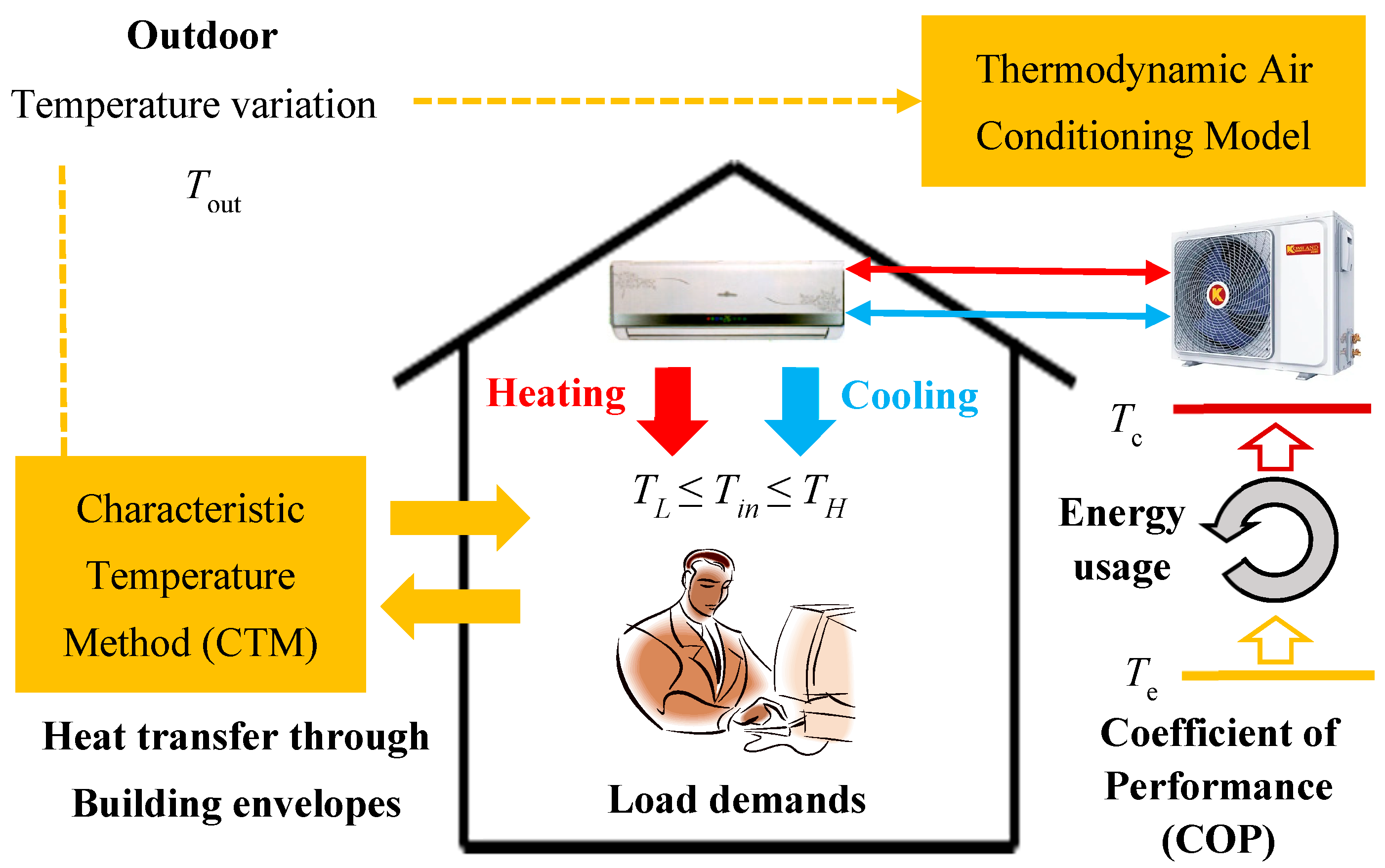
2.1. Building Thermal Model

Figure 1 gives the schematic diagram of a typical air-conditioned built environment. As the introduction stated, the indoor and outdoor temperature variations have coupling impacts on building cooling and heating energy consumptions from two aspects. One is that the indoor–outdoor temperature difference determines the load demands since the dominant cooling and heating loads come from the temperature–difference-driven heat transfer processes through external building envelopes, including walls, windows, roof, etc. The other is that these temperatures determine the air conditioner working condition, especially the evaporation and condensation temperatures (i.e., T_e, T_c), which highly influence the cooling and heating energy efficiency. Thus, to evaluate the dynamic building energy consumptions for indoor cooling and heating, building a thermal model for load simulation needs to be combined with an air conditioner model for efficiency assessment.

The outdoor weather conditions of the office building are based on Chengdu, China, in hot summer and cold winter zone. The Characteristic Temperature Method (CTM) was utilized for the research. Based on the building energy gene theory [29], the dynamic load and energy consumption of buildings are simulated by CTM, and the relationship between load or energy consumption and various other factors can be revealed. According to CTM, if solar radiation gain is considered, the indoor characteristic temperature can be expressed by

$$T_{\mathrm{i}\mathrm{n}}=\frac{\sum K_i{F}_i{T}_{si}+\sum F_{i}I\left({\eta }_i+\frac{{\alpha }_i}{{\alpha }_o}{\rho }_G\right)C_i\mp Q_{\mathrm{A}\mathrm{C}}}{\sum K_i{F}_i}$$

(1)

where $K_i$ is the overall heat transfer coefficient of the building envelope, $\mathrm{W}/\left({\mathrm{m}}^2\cdot \mathrm{K}\right)$; $T_{si}$ is the equivalent solar–air temperature, °C; $F_i$ is the heat transfer area of the model building, ${\mathrm{m}}^2$; $I$ is the global solar radiation intensity, $\mathrm{W}/{\mathrm{m}}^2$; ${\eta }_i$ is the transmittance; ${\rho }_G$ is the absorptivity; $C_i$ is the shading coefficient, and its value is one without any shading measures. $Q_{AC}$ is the provided cooling or heating capacity provided by the air conditioner to maintain the indoor setting temperature within the thermal comfort zone [29]. On the other hand, if not considering solar radiation, $I$ is equal to zero and $T_{si}$ is approximately the outdoor temperature $T_{out}$, °C. Therefore, the expression is changed into

$$T_{\mathrm{i}\mathrm{n}}=\frac{\sum K_i{F}_i{T}_{air}\mp Q_{\mathrm{A}\mathrm{C}}}{\sum K_i{F}_i}$$

(2)

This CTM approach for indoor temperature prediction and building load simulation has been validated in previous studies and verified by commercial building simulation software, including DOE-2, EnergyPlus (Version 2.0), TRNSYS, and DeST (DeST-h 2.0) [30,31,32,33].

2.2. Air Conditioning Model

According to the fundamental principle of thermodynamic cycle (i.e., reverse Carnot circle), an air conditioner such as air-source heat pump can be driven by high grade energy (e.g., electricity) to extract heat from relatively low temperature air, and then release to high temperature heat sink for either space cooling (i.e., evaporation indoor) or heating (i.e., condensation indoor) via the working fluid refrigeration cycling in the device. The thermal performance for such air conditioners can be evaluated by the coefficient of performance (COP), which is defined as the ratio of provided heating or cooling capacity and consumed electricity. Such air conditioning systems have gradually transformed the coal-fired concentrated building energy structure to a more sustainable one with clean and high efficient terminal device applications in China, especially in those expanding big cities with boosting, building, cooling, and heating demands, as well as increasing pressures on resource conservation and environment protection [10]. Therefore, according to the COP definition, timely cooling and heating energy consumption can be expressed by

$${EC}_{\mathrm{A}\mathrm{C}}={EC}_{\mathrm{c}\mathrm{o}\mathrm{o}\mathrm{l}\mathrm{i}\mathrm{n}\mathrm{g}}+{EC}_{\mathrm{h}\mathrm{e}\mathrm{a}\mathrm{t}\mathrm{i}\mathrm{n}\mathrm{g}}={\sum }_{T_{in}>26°\mathrm{C}}^{}\frac{Q_{AC}}{{COP}_{cooling}}+{\sum }_{T_{in}<18°\mathrm{C}}^{}\frac{Q_{AC}}{{COP}_{heating}}$$

(3)

As Equation (3) shows, according to local building design code and indoor thermal comfort standard, the indoor temperature set point (ST) is often 26 °C in summer and 18 °C in winter [9,10]. Therefore, in this paper, the air conditioner is assumed to be activated for cooling if T_in > 26 °C and heating if T_in < 18 °C, respectively. Based on these energy consumption benchmark values, the dynamic cooling and heating energy consumptions can be simulated, respectively, while adjusting the indoor ST under the same characteristics of buildings and meteorological conditions. Under the cooling condition, the load reduction at any time after the ST is raised by 2 °C and the hourly ESR can be obtained based on the cooling load at a ST of 26 °C. The daily, monthly, and yearly ESR can be obtained based on the cooling capacity at the ST of 26 °C. In the same way, under the heating condition, based on the heating load and the heating consumption at the ST of 18 °C, the corresponding ESA and ESR can be obtained while the ST is lowered by 2 °C.

2.3. Illustrative Example

In order to preliminarily illustrate the aforementioned combined CYM-AC model for building energy consumption evaluation, a nine-story office building with a height of 32.4 m located in Chengdu, China, was chosen as the case example here. The case building elevation and plan are shown in Figure 2 and Figure 3, respectively. The characteristics of the building and thermal parameters are shown in

Table 1. Building characteristics and thermal parameters.

Parameters	Value	Unit
total construction area	11,247	m2
total area of the external envelope	7173	m2
building volume	40,727	m3
shape coefficient	0.18
ratio of window to wall (W&E)	0.34
ratio of window to wall (S&N)	0.28
heat transfer coefficient of external wall	1.07	W/m2·K
heat transfer coefficient of external window	3.5	W/m2·K
heat transfer coefficient of roof	0.43	W/m2·K
heat transfer coefficient of ground	1.2	W/m2·K
absorption coefficient of solar radiation to the glazing	0.08
penetration coefficient of solar radiation through the glazing	0.8
shading coefficient	1

.

In the simulation analysis, the demand for cooling and heating loads were calculated, respectively, under the worst conditions. When predicting the cooling load demand, the inner heat source, including personnel, equipment, and lighting, was assumed to be 20 W/m², and the ventilation rate was set at 1.2 h⁻¹. In the calculation, if the outdoor dry bulb temperature is less than the cooling ST, the cooling load should be zero. Because the office building has a small depth, even if there is inner heat source and solar heat gains, the waste heat can be taken away by natural ventilation via opening doors and windows. Only if the outdoor dry bulb temperature and the indoor characteristic temperature are both higher than the cooling ST is there cooling load at that moment. When predicting the heating load demand, the inner heat source, including personnel, equipment, and lighting, was neglected, and the ventilation rate is set at 1.2 h⁻¹. In the thermal modelling, if the outdoor dry bulb temperature and the indoor characteristic temperature are lower than the heating ST, the heating load would be accounted. The working time of office building is from 8:00 to 18:00, and all the moments with cooling or heating load are counted including holidays.

3. Results

3.1. Energy Consumption

3.1.1. Cooling

Figure 4 shows the comparison of the monthly cooling consumption at the ST of 24 °C and 26 °C, respectively. The distribution of them is very similar under the two conditions. The cooling consumption is larger in hot months, smaller in the transition season, and zero in the winter months. When the cooling ST is raised from 24 °C to 26 °C, the monthly cooling consumption will drop significantly. Among them, in April and October, the cooling consumption disappears.

Figure 5 shows the comparison of the monthly and yearly ESA when cooling ST is increased from 24 °C to 26 °C. It can be found that: (1) the cool transition seasons (April and October) have less ESA, and the hotter months (May–September) have more ESA. (2) The change trend of monthly cooling ESA is similar with the change law of monthly cooling consumption shown in Figure 3. Generally, the monthly cooling consumption is higher, the cooling ESA is also higher. Particularly, although the cooling demand in August is the largest, the largest ESA appears in July, the mechanism of which will be revealed later. Figure 6 shows the comparison of the monthly and yearly ESR of the cooling ST from 24 °C to 26 °C. As can be seen, (1) the ESR is higher in the cool transition seasons (April and October), and even reaches 100% in October. The ESR is lower in hotter months (May~September), varying from 15% to 45%. (2) Generally, the higher cooling consumption, the lower ESR. However, there is an exception that the cooling consumption in June is significantly higher than that in May, while ESR is slightly higher than that in May. (3) The yearly cooling ESR is 29%, which is the weighted average of the monthly ESR. And the yearly cooling ESR is closer to the ESR in hotter months.

3.1.2. Heating

Figure 7 shows the comparison of monthly heating consumption at the heating ST of 20 °C and 18 °C, respectively. As can be seen, the distribution of monthly heating energy consumption is very similar under two conditions. The heating consumption is larger in cold winter months, smaller in the transition season, and zero in the summer. When the indoor ST decreases from 20 °C to 18 °C, the monthly heating consumption could be reduced significantly.

Figure 8 shows a comparison of the monthly and yearly ESA of the heating ST being lowered from 20 °C to 18 °C. It can be found that the monthly heating ESA has a significant correlation with the monthly heating consumption. The ESA in the colder months is larger, while in the cooler transition season is smaller. Figure 9 shows a comparison of monthly and yearly ESR of heating ST lowered from 20 °C to 18 °C. The ESR is smaller in the colder months and is larger in the transition seasons. And in June and September, the heating demand will disappear after the heating ST is lowered by 2 °C so that the ESR of the two months is 100%.

3.2. Cooling Energy Saving

In order to further reveal the above-mentioned monthly and yearly energy-saving mechanism of cooling conditions, deep research was conducted from the daily and hourly perspectives, respectively, as follows.

3.2.1. Daily Scale

Figure 10 shows the distribution of daily ESA based on the changes of daily cooling consumption. The horizontal axis is the daily cooling consumption when the cooling ST is 24 °C, and points shown in the figure represent the days with energy-saving effect. There are two distinct phenomena of these points. One is that the daily ESA is proportional to the daily cooling consumption, and the points are arranged in an oblique line, which is counted as 29. The other is that the daily ESA has no obvious distribution law with the increase of daily cooling consumption. The daily ESA ranges from 400 to 3000 kWh, and 94 days of 365 days fall into that situation.

Figure 11 shows the distribution of the daily ESR based on the change of daily cooling consumption before the ST rising 2 °C. Based on the ST of 24 °C, 123 days have cooling need. Among them, 29 days have the ESR of 100%, which means that there would be no need for cooling after increasing the cooling ST. In addition, the overall trend of the other 94 days was revealed. The ESR decreases rapidly with the increase of daily cooling consumption. And the greater the cooling consumption is, the less the ESR changes. From a daily perspective, the mechanism of the monthly and yearly relative ESR can been well-revealed. The monthly ESR shown in Figure 6 is determined by the distribution of daily energy-saving effect in each month. The yearly and monthly cooling ESR is the weighted average of the daily ESR, so the macro ESR is closer to those days with higher daily cooling consumption and the yearly ESR is only 29.4%.

3.2.2. Hourly Scale

Figure 12 shows the variation of the ESA based on the hourly cooling load before the cooling ST rising 2 °C. One point represents one hour with cooling demand. Two distinct distribution rules of ESA are shown with the change of the hourly cooling load. Two kinds of scatter lines are distributed in the figure, and one is close to the horizontal axis. Overall, 708 points are arranged in the horizontal line, and the total ESA is 37,522 kWh, accounting for 22% of the total yearly ESA. The other scatter line is oblique, where the ESA increases with the increase of the hourly cooling load. Only 280 points are arranged in the oblique line and the total ESA accumulated is as high as 132,740 kWh, accounting for 78% of the total yearly ESA. The different distributed characteristic of these moments lead to the different distribution of daily and monthly cooling ESA.

Figure 13 shows the variation of the hourly ESR based on the hourly cooling load before the cooling ST is raised by 2 °C. Among the 988 h with cooling demand of the whole year, the hourly ESR of 280 h is maintained at 100%, which means that these moments will need no cooling after rising the ST. And these points are horizontally distributed in the upper part of the figure, and the scatters in the horizontal line correspond to the oblique line in Figure 12. The ESR of other 708 h decreases slowly with the increase of the hourly cooling load, varying from 0 to 20%, corresponding to the points in the horizontal line in Figure 12. Therefore, from the perspective of hourly ESR distribution, the energy-saving points can be divided into two categories. One is when the ESR is 100%—although the ESR of those points is large, the number is small. However, when the ESR is between 0 and 20%, the number of such points accounts for up to 72% of whole year. The yearly cooling ESR is the weighted average of the hourly ESR, so the ESR rises up to 29.4%, affected by those 100% ESR moments.

3.3. Heating Energy Saving

In order to further reveal the monthly and yearly energy-saving mechanism of heating condition, deep research has been conducted from daily and hourly perspectives, respectively.

3.3.1. Daily Scale

Figure 14 shows the distribution of daily ESA based on the change of daily heating energy consumption. The horizontal axis is the daily heating consumption when the ST is 20 °C, and one point shown in the figure represents the day with heating demand. As can be seen: (1) in the small range of daily heating consumption (0–40 kWh), the daily ESA is proportional to the daily heating consumption, and the scatters are arranged in an oblique line, indicating that 22 days are counted. (2) The daily ESA increases with the rise of daily heating consumption. However, the growth rate of daily ESA gradually slows down when the heating consumption rises. The ESA is spread between 30~300 kWh, and 160 days are counted in this situation. (3) When the daily heating consumption increases from 1100 kWh, the daily ESA is always maintained at around 300 kWh, and 30 days are counted.

Figure 15 shows the distribution of the daily ESR based on the change of daily heating consumption before the ST decreases by 2 °C. Based on the ST of 20 °C, 212 days have heating need. Among them, 22 days have the ESR of 100%, which means that there would be no heating need after decreasing the ST. In addition, the overall trend of the other 190 days is revealed. As the increase of daily heating consumption, the ESR decreases rapidly. And the greater the heating consumption is, the less the ESR changes. From a daily perspective, the mechanism of the monthly and yearly relative ESR can be revealed. The monthly ESR shown in Figure 8 is determined by the distribution of daily energy-saving effect in each month. Following that, the yearly and monthly heating ESR is the weighted average of the daily ESR, so the macro ESR is closer to those days with higher daily heating consumption. The yearly ESR is only 29.4%, which is less affected by the days of 100% ESR.

3.3.2. Hourly Scale

Figure 16 shows the variation of the ESA based on the hourly heating load before the ST drops 2 °C. One point represents one hour with heating demand. Two distinct distribution rules of ESA are shown with the change of the hourly heating load. Two kinds of scatter lines are distributed in the figure. In the range of lower hourly heating load, the hourly ESA is proportional to the hourly heating load, which is presented as an oblique line. Overall, 172 points are arranged in the line, and the total ESA was 2407 kWh, only accounting for 7% of the total yearly ESA. When the hourly heating load increases to a certain value and continues to increase, the hourly ESA is horizontally distributed with a slight upward trend. Overall, 1037 points are arranged in the line and the total ESA accumulated is 28,846 kWh, accounting for 93% of the total yearly ESA. The different distributed characteristic of these moments leads to the different distribution of daily and monthly heating ESA.

Figure 17 shows the variation of the hourly ESR based on the hourly heating load before the ST dropping 2 °C. Among the 1209 h with heating demand of the whole year, the hourly ESR of 172 h is maintained at 100%, and the heating ESR of the other 1037 h decreases exponentially with the increase of the hourly heating load. Therefore, from the perspective of hourly heating ESR distribution, the energy-saving points can be divided into two categories. One category includes the points of 100% ESR, and only 172 h that suits the situation contributes to 7% of the total yearly ESA. The other includes the points when the hourly ESR is less than 100%, and the number of such points accounts for up to 75.6%, contributing 93% of the total yearly ESA. It is the different distributed characteristic of these moments that lead to the different distribution of daily and monthly heating ESR.

4. Discussion: Comparison between Cooling and Heating

Figure 18a,b, respectively, show the change of hourly cooling and heating ESA with the outdoor dry-bulb temperature. As can be seen, although the decreasing range of temperature difference between inside and outside is the same, the micro energy-saving mechanism for cooling and heating is completely different.

As shown in Figure 18a, under the cooling condition, (1) in the range of the cooling ST of 24–26 °C, the energy-saving scatters are arranged in a cylindrical line, where a total of 280 moments are counted and the variation range of ESA is between 200 kWh and 1000 kWh. At the ST of 24 °C, the cooling load of those moments are mainly formed by the indoor heat source and outdoor solar radiation. When the ST is increased artificially, the heat of those can be eliminated by natural ventilation, which is defined as behavioral ESA by the measure itself. And the accumulated ESA of them within the temperature difference range is 132,740 kWh, accounting for 78% of the yearly ESA. (2) In the range where the dry-bulb temperature is more than 26 °C, the energy-saving scatters are arranged in horizontal lines after the ST rises by 2 °C, and 708 points are counted. Every ESA of these moments is very close, about 50 kWh. The ESA is defined as the ESA by temperature difference, and the total value is accumulated as 37,522 kWh, accounting for 22% of the yearly ESA. Therefore, when the cooling ST increases from 24 °C to 26 °C, the energy-saving mechanism of cooling is the main contribution of the yearly ESA: the behavioral ESA by the measure itself, including those moments within the decreasing range of the ST difference, then the secondary contribution is the ESA by temperature difference of the rest moments.

However, it can be seen from Figure 18b that under the heating condition, the distribution of the hourly ESA with the outdoor dry-bulb temperature is completely different from the cooling condition. There are two distinct phenomena, (1) one of which is that the ESA of scatters is between the horizontal axis and the maximum hourly ESA. If the outdoor dry-bulb temperature is between 18 °C and 20 °C, after the ST is lowered by 2 °C, the hourly ESA is equal to the hourly heating load at ST of 20 °C. If the outdoor dry-bulb temperature is much lower than 18 °C, but due to the comprehensive effect of outdoor solar radiation, the indoor characteristic temperature reaches between 18 °C and 20 °C, and the hourly ESA of those moments is also equal to the heating load at a ST of 20 °C. The accumulated ESA of them is 2407 kWh, accounting for 7% of the yearly heating ESA. (2) The other is that when the dry-bulb temperature is lower than 18 °C, the scatters are horizontally distributed. For these moments, the hourly heating consumption depends entirely on the heat transfer coefficient or heat transfer area of building envelope and the decreasing range of temperature difference, but it has no relevance to other parameters. The accumulated ESA of them is 28,846 kWh, accounting for about 93% of the yearly heating ESA. Therefore, when the heating ST is reduced from 20 °C to 18 °C, the energy-saving mechanism of heating is that the main contribution is the ESA by temperature difference, and the secondary contribution comes from the behavioral ESA by the measure itself.

In summary, for the same office building in the same city, the energy-saving mechanism of cooling load or heating load caused by the same energy-saving measure is obviously different. The ESA mainly includes two parts, one of which is the ESA by temperature difference. Another is the behavioral ESA by the measure itself. For cooling, the behavioral ESA is the main contribution of the yearly cooling ESA. For heating, the ESA by temperature difference is the main contribution of the yearly heating ESA.

As Figure 19 shows, in summer, the air conditioner evaporator serves as the indoor unit to provide chilled air, whereas the condenser works outdoors to release heat to an ambient environment. According to the thermodynamic laws, for ideal reverse Carnot cycle, there are T_e = T_in and T_c = T_out, leading to the theoretically maximal energy efficiency COP_i. However, the heat transfer temperature differences (T_e < T_in, T_out < T_c) and other irreversible losses are inevitable for both evaporation and condensation processes in practical engineering fields. For instance, according to local air conditioning design code and standard, the indoor temperature set point is often 26 °C and the outdoor one is about 35 °C in summer. Therefore, the theoretical air conditioner merely needs to work under a relatively narrow temperature change range with a high COP value. Nevertheless, the indoor air supply temperature is often around 12–14 °C, with a much lower practical evaporation temperature for the working fluid inside the equipment (e.g., T_e = 4 °C for Freon refrigerant). On the other hand, the corresponding condensation temperature should exceed the outdoor ambient temperature to facilitate the heat dissipation process outside (e.g., T_c = 40 °C at the cooling tower). As a result, such a temperature difference during heat transfer process significantly degrades air conditioner thermal performance compared to the aforementioned ideal cycle (COP_p < COP_i.). In winter, such an influencing mechanism is similar in terms of shrinking COP values with switched indoor–outdoor unit functions (i.e., T_in < T_c, T_e < T_out) [34,35].

According to the analysis, the building indoor and outdoor temperatures impact not only the cooling and heating load demands inside, but also the operation efficiency of air conditioning systems. These two coupling influence factors significantly determine the practical building air conditioning energy consumptions, with different influence mechanisms and temperature impact sensitivities for cooling and heating, respectively. Previous illustrative examples merely discuss the certain building in Chengdu with given outdoor temperature variations based on China’s building zoning standards, including GB50178-93 “Building Climate Zoning Standard” and GB50176-16 “Civil Building Thermal Design Code”. The division of the architectural climate zone mainly reflects the temporal and spatial distribution characteristics of various basic meteorological elements and their direct impact on the building, reflecting the close relationship between the building and the climate [10]. In order to compare the cooling and heating energy consumptions of the same case building in different climate zones, four typical cities were selected in four different climate zones with both space heating and cooling demands: Harbin, Chengdu, Kunming, and Guangzhou.

Table 2. Key meteorological information of four typical cities in China.

City	Latitude	Longitude	Climatic Region	Mean Temp (°C)	Precipitation (mm)	Solar Radiation (kWh/m2/day)
Harbin	30°40′ N	104°04′ E	Severe Cold	2.92	34.92	3.75
Chengdu	30°40′ N	104°04′ E	Hot Summer and Cold Winter	9.84	79.5	3.16
Kunming	25°03′ N	102°42′ E	Temperate	13.26	83.00	4.19
Guangzhou	23°07′ N	113°15′ E	Hot summer and Warm Winter	20.36	144.83	3.80

shows the key meteorological information.

The case building in Chengdu in Section 2.1 is regarded as the benchmark and reference model. Heating and cooling energy consumptions are investigated with consideration of temperature influencing on both load demands and air conditioning thermal performance. Figure 20 indicates that the annual heating and cooling load proportions vary widely, even for the same case building with identical air conditioning system under different climatic conditions. In Northern China, heating constitutes the dominant part of building air conditioning. For instance, the heating energy consumption of the case building in Harbin can reach 22 kWh/m²y, over ten times its cooling load, and much higher than heating loads in other three cities. For Chengdu and Kunming, located in the Hot Summer and Cold Winter and Temperate climatic regions, respectively, buildings are of relatively close magnitude for cooling and heating load intensity. On the other hand, Guangzhou is the only city of cooling load (15.3 kWh/m²y), significantly exceeding the heating one (1.4 kWh/m²y). Therefore, with consideration of the local climatic parameters, the comparison results illustrate that with the rising city yearly average temperature (i.e., Temperature: Harbin < Chengdu < Kunming < Guangzhou), the heating energy usage increases, whereas cooling consumption decreases. In addition, heating energy consumption seems more sensitive to outdoor temperature variations in China.

5. Conclusions

In summary, a large number of studies have shown that the reasonable choice of ST to reduce indoor–outdoor temperature differences has a significant impact on cooling or heating energy consumption. However, it is not an easy task to make quantitative comparison among all the available research results because they are obtained though case studies under different setting conditions. Researchers often focused on the relative energy-saving ratio (ESR) with temperature change rather than absolute energy-saving amount (ESA), which may make more sense for practical energy usage reduction. In particular, the energy-saving mechanism and temperature influence intensity are different for cooling and heating, even for the same air conditioner (e.g., air-source heat pump). Therefore, a large office building was selected to comparatively analyse its energy-saving effects of indoor–outdoor temperature difference decreasing for cooling and heating, respectively. Moreover, since the climatic conditions, especially outdoor temperature, impact not only the cooling and heating load demands, but also thermal performance and operation efficiency of air conditioning systems, four typical cities located in different climatic zones in China were further chosen as case comparison to investigate the coupling influence of indoor–outdoor temperature difference on energy consumption. The main conclusions are as follows:

(1)

Two types of energy-saving amount (ESA) were designated: heat transfer temperature difference-based ESA and behavioral/operation-based ESA. For heating, the energy-saving mechanism mainly lies in the heat transfer of indoor–outdoor temperature difference, while for cooling, it shifts to behavioral energy saving by rational indoor temperature set-point determination.

(2)

The monthly variations of cooling or heating consumption vary widely. The monthly cooling consumption is higher in summer but lower in the transition seasons and approaches zero in winter. The monthly heating consumption shows an inverse change trend.

(3)

The yearly ESR is the weighted average value of the hourly ESR, which is determined by the hourly distribution of cooling or heating energy-saving effect throughout the year. Therefore, the yearly ESR is closer to the hourly ESR by a large proportion.

(4)

Indoor and outdoor temperatures impact not only the building load demands inside, but also the operation efficiency of air conditioning systems. These two coupling influence factors significantly determine the practical building air conditioning energy consumptions, with different impact sensitivities for cooling and heating, respectively.

(5)

With local climate consideration, the comparison results illustrate that with the rising city yearly average temperature, the heating energy usage increases, whereas cooling consumption decreases. In addition, heating energy consumption seems more sensitive to outdoor temperature variations in China.

The work at this stage simply discusses typical cases to tentatively investigate the household heating and cooling energy-saving mechanism with indoor and outdoor temperatures consideration. When processing and estimating the ESA or ESR values, it will be affected by many practical factors, such as building type, specific air conditioning equipment, dynamic and comprehensive climatic parameters, thermal comfort of the building environment, etc. Such limitations also prompt some future research works for further investigation. This work can provide theoretical support for building energy system design optimization and method reference for the energy-saving analysis of building air conditioning systems with temperature difference considerations for cooling and heating, respectively.

References

- Gaglia, A.G.; Dialynas, E.N.; Argiriou, A.A. Energy performance of European residential buildings: Energy use, technical and environmental characteristics of the Greek residential sector—Energy conservation and CO2 reduction. Energy Build. 2019, 183, 86–104. [Google Scholar] [CrossRef]
- Al-Marri, W.; Al-Habaibeh, A.; Watkins, M. An investigation into domestic energy consumption behaviour and public awareness of renewable energy in Qatar. Sustain. Cities Soc. 2018, 41, 639–646. [Google Scholar] [CrossRef]
- Bourdeau, M.; Zhai, X.Q.; Nefzaoui, E.; Guo, X.F.; Chatellier, P. Modeling and forecasting building energy consumption: A review of data-driven techniques. Sustain. Cities Soc. 2019, 48, 101533. [Google Scholar] [CrossRef]
- Gao, H.; Koch, C.; Wu, Y.P. Building information modelling based building energy modelling: A review. Appl. Energy 2019, 238, 320–343. [Google Scholar] [CrossRef]
- Pokhrel, R.; Gonzalez, J.E.; Ramamurthy, P.; Comarazamy, D. Impact of building energy mitigation measures on future climate. Atmosphere 2023, 14, 463. [Google Scholar] [CrossRef]
- Ding, P.; Li, J.; Xiang, M.L.; Cheng, Z.; Long, E.S. Dynamic heat transfer calculation for ground-coupled floor in emergency temporary housing. Appl. Sci. 2022, 12, 11844. [Google Scholar] [CrossRef]
- Darlington Mushore, T.; Odindi, J.; Dube, T.; Mutanga, O. Understanding the relationship between urban outdoor temperatures and indoor air-conditioning energy demand in Zimbabwe. Sustain. Cities Soc. 2017, 34, 97–108. [Google Scholar] [CrossRef]
- Carreira, P.; Aguiar Costa, A.; Mansur, V.; Arsénio, A. Can HVAC really learn from users? A simulation-based study on the effectiveness of voting for comfort and energy use optimization. Sustain. Cities Soc. 2018, 41, 275–285. [Google Scholar] [CrossRef]
- Zheng, Y.H.; Si, P.F.; Zhang, Y.; Shi, L.J.; Huang, C.J.J.; Huang, D.S.; Jin, Z.N. Study on the effect of radiant insulation panel in cavity on the thermal performance of broken-bridge aluminum window frame. Buildings 2023, 13, 58. [Google Scholar] [CrossRef]
- Jin, Z.N.; Zheng, Y.H.; Zhang, Y. A novel method for building air conditioning energy saving potential pre-estimation based on thermodynamic perfection index for space cooling. J. Asian Archit. Build. Eng. 2023, 22, 2348–2364. [Google Scholar] [CrossRef]
- Qi, X.Y.; Zhang, Y.; Jin, Z.N. Building energy efficiency for indoor heating temperature set-point: Mechanism and case study of mid-rise apartment. Buildings 2023, 13, 1189. [Google Scholar] [CrossRef]
- Moreci, E.; Ciulla, G.; Lo Brano, V. Annual heating energy requirements of office buildings in a European climate. Sustain. Cities Soc. 2016, 20, 81–95. [Google Scholar] [CrossRef]
- Park, Y.S.; Jeong, J.H.; Ahn, B.H. Heat pump control method based on direct measurement of evaporation pressure to improve energy efficiency and indoor air temperature stability at a low cooling load condition. Appl. Energy 2014, 132, 99–107. [Google Scholar] [CrossRef]
- Yang, B.; Sekhar, C.; Melikov, A.K. Ceiling mounted personalized ventilation system in hot and humid climate—An energy analysis. Energy Build. 2010, 42, 2304–2308. [Google Scholar] [CrossRef]
- Hoyt, T.; Arens, E.; Zhang, Z.H. Extending air temperature setpoints: Simulated energy savings and design considerations for new and retrofit buildings. Build. Environ. 2015, 88, 89–96. [Google Scholar] [CrossRef]
- Aynsley, R. Quantifying the cooling sensation of air movement. Int. J. Vent. 2008, 7, 67–76. [Google Scholar] [CrossRef]
- Walikewitz, N.; Janicke, B.; Langner, M.; Meier, F.; Endlicher, W. The difference between the mean radiant temperature and the air temperature within indoor environments: A case study during summer conditions. Build. Environ. 2015, 84, 151–161. [Google Scholar] [CrossRef]
- Munoz, F.; Sanchez, E.N.; Xia, Y.D.; Deng, S.M. Real-time neural inverse optimal control for indoor air temperature and humidity in a direct expansion (DX) air conditioning (A/C) system. Int. J. Refrig. 2017, 79, 196–206. [Google Scholar] [CrossRef]
- Yan, H.X.; Xia, Y.D.; Deng, S.M. Simulation study on a three-evaporator air conditioning system for simultaneous indoor air temperature and humidity control. Appl. Energy 2017, 207, 294–304. [Google Scholar] [CrossRef]
- Yan, H.X.; Xia, Y.D.; Xu, X.D.; Deng, S.M. Inherent operational characteristics aided fuzzy logic controller for a variable speed direct expansion air conditioning system for simultaneous indoor air temperature and humidity control. Energy Build. 2018, 158, 558–568. [Google Scholar] [CrossRef]
- Ghahramani, A.; Zhang, K.; Dutta, K.; Yang, Z.; Becerik-Gerber, B. Energy savings from temperature setpoints and deadband: Quantifying the influence of building and system properties on savings. Appl. Energy 2016, 165, 930–942. [Google Scholar] [CrossRef]
- Asif, A.; Zeeshan, M.; Jahanzaib, M. Indoor temperature, relative humidity and CO2 levels assessment in academic buildings with different heating, ventilation and air-conditioning systems. Build. Environ. 2018, 133, 83–90. [Google Scholar] [CrossRef]
- Wang, D.J.; Xu, Y.C.; Liu, Y.F.; Wang, Y.Y.; Jiang, J.; Wang, X.W.; Liu, J.P. Experimental investigation of the effect of indoor air temperature on students’ learning performance under the summer conditions in China. Build. Environ. 2018, 140, 140–152. [Google Scholar] [CrossRef]
- Bekdas, G.; Aydin, Y.; Isikdag, U.; Sadeghifam, A.N.; Aidin, N.; Kim, S.; Geem, Z.W. Prediction of cooling load of tropical buildings with machine learning. Sustainability 2023, 15, 9061. [Google Scholar] [CrossRef]
- Li, Y.Y.; Li, H.J.; Miao, R.; Qi, H.; Zhang, Y. Energy-Environment-Economy (3E) analysis of the performance of introducing photovoltaic and energy storage systems into residential buildings: A case study in Shenzhen, China. Sustainability 2023, 15, 9007. [Google Scholar] [CrossRef]
- Sibill, M.; Touibi, D. Abanda FH, Rethinking abandoned buildings as positive energy buildings in a former industrial site in Italy. Energies 2023, 16, 4503. [Google Scholar] [CrossRef]
- Adsetts, J.R.; Ebrahimi, N.; Zhang, J.Y.; Jalaei, F.; Noel, J.J. Improving the energy efficiency of public utility buildings in Poland through thermomodernization and renewable energy sources—A case study. Coatings 2023, 13, 850. [Google Scholar] [CrossRef]
- Hung, L.C.; Pan, N.H. Thermal stability, kinetic analysis, and safe temperature assessment of ionic liquids 1-Benzyl-3-Methylimidazolium Bis (Trifluoromethylsulfonyl) imide for emerging building and energy related field. Processes 2023, 11, 1121. [Google Scholar] [CrossRef]
- Long, E.S. Research on the influence of air humidity on the annual heating or cooling energy consumption. Build. Environ. 2005, 40, 571–578. [Google Scholar]
- Guo, S.R.; Yang, H.Y.; Li, Y.R.; Zhang, Y.; Long, E.S. Energy saving effect and mechanism of cooling setting temperature increased by 1 °C for residential buildings in different cities. Energy Build. 2019, 202, 109335. [Google Scholar] [CrossRef]
- Li, Y.R.; Long, E.S.; Jin, Z.H.; Li, J.; Meng, X.; Zhou, J.; Xu, L.T.; Xiao, D.T. Heat storage and release characteristics of composite phase change wall under different intermittent heating conditions. Sci. Technol. Built Environ. 2019, 25, 336–345. [Google Scholar] [CrossRef]
- Xu, L.T.; Long, E.S.; Wei, J.C. Study on the limiting height of rooftop solar energy equipment in street canyons under the cityscape constraints. Sol. Energy 2020, 206, 1–7. [Google Scholar] [CrossRef]
- Li, J.; Zhang, Y.; Ding, P.; Long, E.S. Experimental and simulated optimization study on dynamic heat discharge performance of multi-units water tank with PCM. Indoor Built Environ. 2021, 30, 1531–1545. [Google Scholar] [CrossRef]
- Deng, J.W.; Wei, Q.P.; Liang, M.; He, S.; Zhang, H. Does heat pumps perform energy efficiently as we expected: Field tests and evaluations on various kinds of heat pump systems for space heating. Energy Build. 2019, 182, 172–186. [Google Scholar] [CrossRef]
- Xu, Z.W.; Li, H.; Shao, S.Q.; Xu, W.; Wang, Z.C.; Gou, X.X.; Zhao, M.Y.; Li, J.D. Investigation on the efficiency degradation characterization of low ambient temperature air source heat pump under partial load operation. Int. J. Refrig. 2021, 133, 99–110. [Google Scholar] [CrossRef]