Remote Sensing Study on the Coupling Relationship between Regional Ecological Environment and Human Activities: A Case Study of Qilian Mountain National Nature Reserve

Abstract

Analyzing human–environment coupling is important in understanding the mechanisms and developments of human–environment systems. However, the current frameworks and approaches evaluating the relationship between human activities and the ecological environment remain limited. Integrating the vegetation-impervious surface–soil–air framework, Mann–Kendall test, correlation analysis, two-step floating catchment area method, coupling analysis, and optimal parameters-based geographical detector, this study comprehensively evaluate the environmental changes and analyzes the coupling relationship between environment and human activities, mainly in terms of habitat quality, landscape pattern, and ecological services. The study area was the Qilian Mountain National Nature Reserve in Gansu province, China, an ecologically fragile region with an environment closely linked to human activities. Along with district and county census data, various remote-sensing products (e.g., MODIS, Landsat) were used to assess the ecological level and human–environment coupling state of the study site from 2003 to 2019. The main results show: (1) The remote sensing composite index, which integrates eight ecological sub-indices, effectively captures the spatial and temporal variations of the ecological environment in the study area, providing comprehensive and detailed environmental information. (2) Analysis using the Mann–Kendall-correlation classification, coupling degree, and two-step floating catchment area methods consistently demonstrates a gradual coordination between human activities and the ecological environment in the study area. (3) In comparison to spatially interpolated population data, the remote sensing human activity index more significantly represents the spatial impact of human activities on the ecological environment. (4) The environmental aspects most strongly associated with human activities include carbon fixation and oxygen release, vegetation, humidity, and soil. (5) The ecological environment level does not uniformly deteriorate with increasing population density, and a notable alignment is observed between changes in the ecological environment and the implementation of government environmental protection policies.

1. Introduction

With the rapid urbanization and industrialization since the 20th century, the impact of human activities on the ecological environment has become more serious. Anthropogenic activities have considerable effects on the ecological environment in various aspects. Industrial production can significantly increase air, water, and soil pollution [1,2,3]. Excessive human interference can also lead to natural disasters in ecologically vulnerable areas [4] and cause large-scale environmental changes (e.g., climate change) [5].

The ecological environment has a close and complex coupling relationship with anthropogenic activities [6]. The mechanisms underlying the impact of human activities on the ecological environment remain inadequately elucidated. Puzzlingly, there are cases in which ecological degradation persists despite the reduction in human activities, deviating from conventional expectations [7]. To reduce damage and maintain sustainable development in the ecological environment, the coupling mechanism between human activities and the ecological environment should be further explored.

A comprehensive evaluation and scientific cognition of the ecological environment is crucial to understand better the coupling mechanism of human activities and the environment. Remote sensing technology has gradually become an important tool for ecological monitoring due to its advantages, such as a large coverage area and short data acquisition period [8,9]. Remote sensing monitoring involves obtaining long time series of land use, vegetation cover, temperature, and humidity index, which are important in comprehensively evaluating the ecological environment [10].

The coupling between human activities and the ecological environment refers to the process of interaction and mutual influence between human society and the natural environment. This interaction is bidirectional, including both the impact of humans on the natural environment and the impact of the natural environment on human society. This coupling relationship is a complex system that includes many different levels and factors, such as the economy, society, culture, technology, ecology, and environment [11]. Since the 1960s, numerous studies have used remote sensing data to explore and create various models and index systems for ecological environmental assessment [12], developing new simulation and evaluation approaches, such as the analytic hierarchy process [13], fuzzy evaluation method [14], principal component analysis method [15], grey assessment model [16], and artificial neural networks [17]. For example, Xu et al. integrated four ecological quality indicators to build a composite index for environmental evaluation based on the pressure state response framework, monitoring ecological change using change vector analysis (CVA) [18]. Liu et al. calculated landscape pattern indexes with FRAGSTATS software and evaluated the relationship between environmental pollution and landscape pattern using redundancy analysis (RDA) [19,20,21]. With further developments in geospatial technology, environmental modeling, and spatial data infrastructure, the comprehensive selection and evaluation of ecological factors and the appropriate approaches to integrate them have become major frontiers in ecological evaluation research [22].

The coupling relationship between human activities and ecological environment has been given much attention by international scholars. For example, Fu et al. used the coupling coordination model to quantitatively evaluate the coupling relationship between urbanization and the ecological environment in Qingdao during 2000–2018 [23]. Huang et al. analyzed the coupling characteristics of human activity intensity and landscape pattern in the Three Gorges Reservoir area and the evolution of the man–land relationship in the region [24]. Zhang et al. constructed the evaluation index system of the production–living–ecological space (PLES) functional system in China’s underdeveloped areas and used the coupling coordination degree model to measure the development coordination level [25]. Research on human–environment coupling has gradually shifted from evaluating a single index or partial factor coupling to creating a network system covering many ecological factors and comprehensively analyzing their interaction mechanism with human activities [26,27]. Furthermore, several research theories, models, and frameworks have been proposed on the mechanism between human activities and the ecological environment [28,29,30,31].

However, in most studies evaluating the local ecological environment, the indicators are often limited to one habitat quality, landscape pattern, and ecological service, preventing a more comprehensive cognition of the state of the ecological environment [32,33,34,35,36]. And, while several studies have used multiple methods to make extensive analyses and comparisons [37], the approaches to analyzing the coupling of the ecological environment and human activities need to be integrated and improved. The single-analysis method not only made the conclusion less convincing, but also made it difficult to fully recognize the coupling law between human activities and ecological environment.

Taking Qilian Mountain National Nature Reserve as an example, the ecological factors covered in a single ecological assessment are insufficient to develop the region’s environmental assessment network. The current research content needs to be further supplemented and discussed in the collective evolution of human activities and the ecological environment in the Qilian Mountains. To address some of the knowledge gaps, this study integrated the ecological factors of habitat quality, ecological service, and landscape pattern into a comprehensive ecological evaluation of the Qilian Mountain Reserve from 2003 to 2019. This paper also interprets the coupling state between human activities and ecological environment from another perspective by combining the Mann–Kendall test with correlation analysis. The coupling evolution of the ecological environment and human activities is preliminarily described by cross-validation with the results of other coupling analysis methods.

2. Materials and Methods

2.1. Study Area

Qilian Mountain National Nature Reserve (Figure 1) is a forest and wildlife-type national nature reserve established in 1988. It is located at the northern foot of the Qilian Mountains at the intersection of the Qinghai–Tibet Plateau, the Mongolian–Xinjiang Plateau, and the Loess Plateau. The natural protected areas in Gansu Province range from 97.4° E to 103.5° E and 36.9° N to 39.6° N, with a total area of about 2.653 million hectares. The Qilian Mountains National Nature Reserve has a continental alpine and semi-humid mountain climate, with an average annual precipitation of 257.2~389.9 mm concentrated from May to September and an average annual temperature of 1.0~4.0 °C.

The western section has a moderate-to-severe fragile natural ecosystem. The middle part is mainly alpine meadow, with high terrain, low temperature, rainy climate, and high vegetation coverage, and has a moderately fragile natural system. The eastern section is mainly temperate grasslands, with relatively low terrain and low vegetation coverage, and has a mild-to-moderate fragile ecosystem [38]. Qilian Mountain National Nature Reserve includes the Sunan Autonomous Prefecture, Tianzhu Autonomous Prefecture, Gulang County, Shandan County, Qilian County, Liangzhou District, and the Ganzhou District.

2.2. Data Sources

Various images obtained from the Google Earth Engine (GEE) platform were used to evaluate and analyze the ecological level. Before synthesizing the annual data, the study utilized quality control bands of remote sensing products (such as the StateQA band of MOD09A1) to remove the values of pixels with poor quality throughout the year (such as those covered by clouds). In order to obtain a representative image for a given year of a remote sensing product, we adopted a methodology of selecting the median value of each pixel across all images within that year in the GEE platform and synthesizing them into a single image. This representative image was then used to represent the product for that year in subsequent calculations. After resampling all images with resolutions lower than 500 m to a resolution of 500 m using ArcGIS and cropping them to a uniform row and column number, subsequent processing and calculations were carried out using IDL, as well as the GDAL and numpy libraries of Python (

Table 1. The data sources of ecological evaluation sub-indicator.

Data Name (E/C)	Data Source	Resolution	Time Range
NDBSI (C)	MOD09A1.006:Terra Surface Reflectance 8-Day Global 500 m	500 m/8-day	2003–2019
LST (E)	MOD11A2.006:Terra Land Surface Temperature and Emissivity 8-Day Global 1 km	1000 m/8-day	2003–2019
AOD (E)	MCD19A2.006:Terra and Aqua MAIAC Land Aerosol Optical Depth Daily 1 km	1000 m/1-day	2003–2019
EVI (E)	MOD13A2.006:Terra Vegetation Indexes 16-Day Global 1 km	1000 m/16-day	2003–2019
WET (C)	MOD09A1.006:Terra Surface Reflectance 8-Day Global 500 m	500 m/8-day	2003–2019
LC (E)	MCD12Q1.006:MODIS Land Cover Type Yearly Global 500 m	500 m/1-year	2003–2019
AI (C)	Annual China Land Cover Dataset (CLCD)	30 m/1-year	2003–2019
Qtco2/Qop (C)	MOD17A3HGF.006:Terra Net Primary Production Gap-Filled Yearly Global 500 m	500 m/8-day	2003–2019
ET (E)	MOD16A2.006:Terra Net Evapotranspiration 8-Day Global 500 m	500 m/8-day	2003–2019
Fpar (E)	MCD15A3H.006:MODIS Leaf Area Index/FPAR 4-Day Global 500 m	500 m/4-day	2003–2019
Qsor (E)	RADI_MUL_CHN_DAY	meteorological station/1-day	2003–2019
NDVI (E)	MOD13A1.006:Terra Vegetation Indexes 16-Day Global 500 m	500 m/16-day	2014–2019
NTL (E)	VIIRS Stray Light Corrected Nighttime Day/Night Band Composites Version 1	15 arc seconds/1-month	2014–2019
Population Density (E)	demographic census	500 m	2003, 2010, 2019

‘E’ in parentheses represents data from existing remote sensing products or other publicly available data. ‘C’ in parentheses represents data calculated from multiple remote sensing products or other publicly available data.

, Figure 2).

2.3. Methods

2.3.1. Summary of Research Method

Eight ecological evaluation sub-indexes were selected from the aspects of habitat quality, landscape pattern, and ecological services (see Figure 3). The required data images were downloaded and processed using GEE and other platform tools. Integrating meteorological station data from 2003 to 2019, the median images for each ecological sub-index were obtained, with a unified resolution of 500 m. Pixels with permanent snow and ice cover or affected by clouds were removed to reduce errors.

The applicability of ecological sub-indicators for factor analysis in each year was evaluated using the KMO test and Bartlett’s sphericity test. Subsequently, principal component analysis (PCA) was used to reduce the dimensionality of the eight ecological sub-indicators into a Remote Sensing Composite Index (RSCI) and analyze the environmental trends in the study area. The Mann–Kendall (MK) test was used to screen out pixels with abrupt changes in ecological level, and the correlation between the RSCI Index and the Human Settlement Index (HSI) was calculated to assess the impact of human activities on ecological conditions [39]. The Ecological Spatial Accessibility Index (ESAI) of RSCI was also computed using the Two-Step Floating Catchment Area Method (2SFCA) [40]. By analyzing the results of the three methods, the relationship and interactions of human activities and the ecological environment in the Qilian Mountain Reserve can be better understood.

2.3.2. Calculation Method of Ecological Evaluation Sub-Index

1.

Habitat quality sub-index

The habitat quality metric in the study was based on the vegetation-impervious surface–soil–air (VISA) framework [41]. The VISA framework is an improvement on the traditional vegetation-impervious surface–soil (VIS) framework, taking into account the impact of air pollution on the ecological environment. The ecological evaluation parameters used in assessing habitat quality were the normalized differential build-up and bare soil index (NDBSI), land surface temperature (LST), aerosol optical depth (AOD), enhanced vegetation index (EVI), and wetness (WET).

In addition to LST, which adopts a split-window algorithm product [42], other sub-indexes were obtained using the MODIS surface reflectance product for band operation. The bands involved include the red band (${\rho }_{red}$), the near-infrared band (${\rho }_{red}$), the short infrared band (${\rho }_{\mathrm{swir}}$), the green band (${\rho }_{green}$), the blue band (${\rho }_{blue}$), and the thermal infrared band (${\rho }_{tir}$).

The calculation formula of NDBSI is:

$$NDBSI=\left(IBI+SI\right)/2$$

(1)

where

$$\begin{array}{c}SI=\frac{\left({\rho }_{swir1}+{\rho }_{red}\right)-\left({\rho }_{nir}+{\rho }_{blue}\right)}{\left({\rho }_{swir1}+{\rho }_{red}\right)+\left({\rho }_{nir}+{\rho }_{blue}\right)}\\ IBI=\frac{2v_{swir1}-v_{nir}+v_{green}}{2v_{swir1}+v_{nir}+v_{green}}\\ v_{swir1}={\rho }_{swir1}/\left({\rho }_{swir1}+{\rho }_{nir}\right)\\ v_{nir}={\rho }_{nir}/\left({\rho }_{nir}+{\rho }_{red}\right)\\ v_{green}={\rho }_{green}/\left({\rho }_{green}+{\rho }_{swir1}\right)\end{array}$$

(2)

There are blue band and green band AODs over land in MCD19A2. The average AOD index can be calculated using the formula:

$$AOD=\left({\rho }_{green}+{\rho }_{blue}\right)/2$$

(3)

The calculation formula of EVI is:

$$EVI=2.5\frac{{\rho }_{nir}-{\rho }_{red}}{{\rho }_{nir}+6{\rho }_{red}-7.5{\rho }_{blue}+1}$$

(4)

The calculation formula of WET is:

$$\begin{array}{c}WET=0.1147\times {\rho }_{red}+0.2489\times {\rho }_{nir}\\ +0.2408\times {\rho }_{blue}+0.3132\times {\rho }_{green}\\ -0.3122\times {\rho }_{tir}-0.6416\times {\rho }_{swir1}\\ -0.5087\times {\rho }_{swir2}\end{array}$$

(5)

2.

Landscape pattern sub-index

In landscape ecology, quantifying landscape patterns is crucial for establishing the link between spatial patterns and ecological processes. Quantification of spatial landscape pattern aggregation level serves as an important step in connecting landscape patterns with ecological processes and is one of the key indicators for assessing the level of ecological environment [43].

The degree of landscape aggregation index (AI) was selected as the landscape pattern evaluation index to evaluate the connectivity between patches of each landscape type [44]. The landscape indicators were mainly obtained using FRAGSTATS software (http://www.umass.edu/landeco/research/fragstats/fragstats.html, (accessed on 3 February 2023)). While it can provide the AI value for a particular landscape in the image, they are unable to fully meet the research needs. The AI values had to be refined to pixel scale. Based on the land cover image with 30 m resolution, the adjacent 17 × 17 grid pixels were taken as a new pixel (approximately 500 m × 500 m) for analysis. The AI value of the corresponding landscape was calculated according to the distribution of nine landscape types (e.g., forest, grassland, shrub) in the new pixel, and the maximum value of the nine AI values was selected as the final pixel value.

$$AI=\left[\underset{\max \to g_{ij}}{g_{ij}}\right]\times 100$$

(6)

where $g_{ij}$ is the aggregation degree of similar adjacent patches of this type of landscape, and correlation conversion is carried out based on the length of common edges of patches of the same type.

3.

Ecological services sub-index.

The carbon sequestration and oxygen release (Qop/Qtco₂) and the climate regulatory capacity (CRC) sub-indexes were used for the ecological service evaluation. The calculation method is referred to The Technical Guideline on Gross Ecosystem Product (GEP) published by Chinese Academy of Environmental Planning. The carbon sequestration and oxygen release capacity was determined using the net ecosystem productivity method:

$$Q_{tC{O}_2}=\left(M_{C{O}_2}/M_C\right)\times \alpha \times NPP\times \left(M_{C_6}/M_{C_6{H}_{10}{O}_5}\right)$$

(7)

$$Q_{op}=\left(M_{O_2}/M_{C{O}_2}\right)\times Q_{tC{O}_2}$$

(8)

where NPP is net primary productivity; $\alpha$ is the conversion coefficient for net ecosystem productivity (NEP) and NPP depending on ecosystem type; $M_{C_6}/M_{C_6{H}_{10}{O}_5}$ is the coefficient of conversion of C to CO₂; $M_{C{O}_2}/M_C$ is the coefficient of conversion for dry matter to C; $M_{O_2}/M_{C{O}_2}$ is the coefficient of conversion of CO₂ to O₂.

CRC is evaluated using the solar energy absorbed by the ecosystem through the processes of vegetation transpiration and water surface evaporation.

$$CRC=\left(ET\times hlg\right)-{\displaystyle \sum _{i=1}^{365}\left(Q_{so{r}_i}\times FPA{R}_i\right)}$$

(9)

where ET is the annual evapotranspiration; hlg is the latent heat of steam and evaporation for 0.1 MPa atmospheric pressure; $Q_{so{r}_i}$ is the daily total net radiation; $FPA{R}_i$ is the daily plant absorbable photosynthetically active radiation component.

The daily net radiation data used in this study were obtained from the official website of the National Meteorological Science Data Center of China. The only site with relatively complete data in the study area was the Lanzhou station (station number 52889/52983). For each year, all available Fpar images based on MODIS data were collected and matched to the daily net radiation data between the two time points (usually four days) of the two Fpar images. The data were then calculated and summed.

2.3.3. Evaluation of Comprehensive Ecological Index

The eight ecological evaluation sub-indexes selected from habitat quality, landscape pattern, and ecological services were integrated using principal component analysis (PCA) to obtain the comprehensive ecological index RSCI. The calculation method is as follows:

$$RSCI=f\left(AOD,EVI,LST,NDBSI,WET,AI,CRQ,Q_{op}/Q_{tc{o}_2}\right)$$

(10)

First, hyperbolic tangent normalization is carried out for each sub-index:

$$\{\begin{array}{c}{Z}_i=\begin{array}{cc}\left(x_i-\mu \right)/\sigma & if i is a positive index\end{array}\\ Z_i=\begin{array}{cc}\left(\mu -x_i\right)/\sigma & if i is a negative index\end{array}\\ I_i=\left(e^{Z_i}-e^{-Z_i}\right)/\left(e^{Z_i}+e^{-Z_i}\right)\end{array}$$

(11)

where $x_i$ is the pixel value of the positive/negative index; $\mu$ is the average value of all pixel values of the positive/negative indicator; $\sigma$ is the standard deviation of all pixel values of the positive/negative index; $Z_i$ is the z-score standardized result of this index; $I_i$ is the final hyperbolic tangent normalized result, [−1, 1].

The RSCI can be calculated based on the normalized results of each sub-index:

$$RSCI={\displaystyle \sum _{i=1}^8{w}_i\times I_i}$$

(12)

where $w_i$ is the weight of a positive/negative index in the RSCI, determined by PCA. The formula for $w_i$ is as follows:

$$\{\begin{array}{c}{w}_i=H_i/{\displaystyle {\sum }_{i=1}^8{H}_i}\\ H_i={\displaystyle {\sum }_{j=1}^m{\left({\lambda }_{i,j}\right)}^2}\end{array}$$

(13)

where ${\lambda }_{i,j}$ is the factor loading of the ith positive/negative index in the jth principal component; m is the number of principal components with cumulative contribution greater than 95%; $H_i$ is the common factor variance of the ith index.

2.3.4. Coupling of Ecological Index and Human Activity Index

The coupling of ecological conditions and human activities in the Qilian Mountains was analyzed from two perspectives:

• Integrating MK test and correlation analysis

Based on the MK test [45], the pixels with a significant upward or downward trend of RSCI were screened out. Pearson correlation coefficient was then used to analyze the correlation between RSCI and the human settlements index [46] and evaluate the impact of human activities on the ecological environment. The calculation formula for HSI is as follows:

$$HSI=\frac{\left(1-NDV{I}_{\max }\right)+NT{L}_{nor}}{\left(1-NT{L}_{nor}\right)+NDV{I}_{\max }+NT{L}_{nor}\times NDV{I}_{\max }}$$

(14)

where HSI is the human settlements index; $NDV{I}_{\max }$ is the normalized difference vegetation index; $NT{L}_{nor}$ is the normalized night light index.

2.

Analysis of coupling degree and ecological spatial accessibility

The Ecological Spatial Accessibility Index (ESAI) was calculated at pixel scale to evaluate the ecological welfare of local residents within their normal activity range (radius 3 km–10 km). Using county census data and Inverse Distance Weight (IDW) method, 500 m raster data were obtained. The raster data and RSCI images for 2003, 2010, and 2019 were combined to calculate the index using the Two-Step Floating Catchment Area Method (2SFCA). The calculation method is divided into two steps as follows:

First, for pixel j, all pixels (k) within the range of the threshold of distance from j ($d_0$, 3 km for walking, and 10 km for driving) are searched through traversal to calculate the supply and demand ratio of pixel j ecological value ($R_j$):

$$R_j=\frac{RSC{I}_j}{{\displaystyle \sum _{k\in \left\{d_{kj}\le d_0\right\}}{P}_k}}$$

(15)

where $RSC{I}_j$ is the ecological composite index of j pixel; $d_{kj}$ is the straight-line distance between the center point of k pixel and j pixel; $P_k$ is the population density of k pixels.

Then, the ESAI of pixels is calculated based on $R_j$ traversal:

$$ESA{I}_i={\displaystyle \sum _{j\in \left\{d_{ij}\le d_0\right\}}{R}_j}$$

(16)

where $d_{ij}$ is the straight-line distance between the center points of pixels i and j; $R_j$ is the ratio of supply and demand of pixel j’s ecological value.

In addition, by analyzing the coupling degree (C) of RSCI, ESAI and population density (PD), the study also analyzes the coordination degree of coupling evolution between human activities and ecological conditions [47]. The calculation formula is as follows:

$$C=\sqrt{\frac{RSCI\times PD}{{\left[\frac{RSCI+PD}{2}\right]}^2}}$$

(17)

3. Results

3.1. Comprehensive Ecological Status Analysis

Based on the hyperbolic tangent normalization statistics (see Figure 4), all sub-indexes were found to have an upward trend from 2003 to 2019, among which AOD, LST, CRC, and Qop/Qtco₂ indexes showed the most pronounced growth. The main landscape types were grassland, bare soil, farmland, and forest, with pixel proportions of 75.62%, 9.11%, 8.12%, and 6.14%, respectively.

The weight of each sub-index was determined by PCA. The results (Figure 4) show that the weight distribution of the eight sub-indexes was relatively uniform, and the weight of AI, NDBSI, CRC, and Qop/Qtco₂ in RSCI was slightly higher. The overall data have good orthogonality, which reflects the reasonable selection of indicators.

In addition, the coefficients of sensitivity (CS) of each ecological sub-index to RSCI were calculated by numerical perturbation in the range of 50% [48]. The results showed that RSCI was more sensitive to the changes of LST, WET, and CRC when the value of sub-index increased, while RSCI was most sensitive to the changes of AI when the value of sub-index decreased.

The RSCI results from 2003 to 2019 in Figure 4 show that the average ecological level had a fluctuating upward trend, with the highest normalized value at 0.649 in 2017 and the lowest normalized value at 0.513 in 2004 (Figure 5). The comprehensive ecological index for Sunan Autonomous County, Tianzhu Autonomous County, and Qilian County in the southwest was high, and low in the northwest of Sunan Autonomous County, northeast of Liangzhou, Gulang, and other areas.

The Mann–Kendall test results in Figure 6 show that, from 2003 to 2019, the RSCI indexes in most areas (72.20%) had a significant upward trend, and the spatial distribution was relatively uniform. Pixels with weak significant increase (statistical value higher than 1.28) accounted for 7.18%, while those with strong significant increase (statistical value higher than 1.64) accounted for 20.09%. Areas with high significant increase (statistical value higher than 2.32) comprised 50.65%, while those with no significant change accounted for 20.62%. However, the proportion of pixels that had significant declines in RSCI was only 1.46%, scattered in the northwest, central, and southwest corners.

The mutation years for each pixel during 2014–2019 were determined by calculating the statistics curve of the MK test in reverse and determining its intersection with the positive statistics curve (Figure 7).

As shown in

Table 2. MK mutation year.

Year of Mutation (Significant Decrease)	Number of Pixels	Year of Mutation (Significant Increase)	Number of Pixels
2004	531	2019	18,738
2005	205	2017	10,336
2006	94	2015	5817
2009	65	2014	4546
2010	31	2016	3556
2008	17	2013	3201
2011	14	2018	2869
2013	12	2012	2630
2007	10	2010	830
2012	7	2011	546
2016	6	2009	297
2015	6	2007	138
2014	2	2008	97
		2006	12

, the mutation years of RSCI in the Qilian Mountain Reserve from 2003 to 2019 (significant increase) were mainly in 2019 and 2017. The regions with 2017 as the year of mutation were concentrated primarily on the mid-abdomen part, while those with the year of mutation in 2019 were situated mainly in Gulang County, Sunan Autonomous Prefecture, and Tianzhu Autonomous Prefecture in the southeast.

3.2. Coupling Analysis of Ecological Status and Human Activities

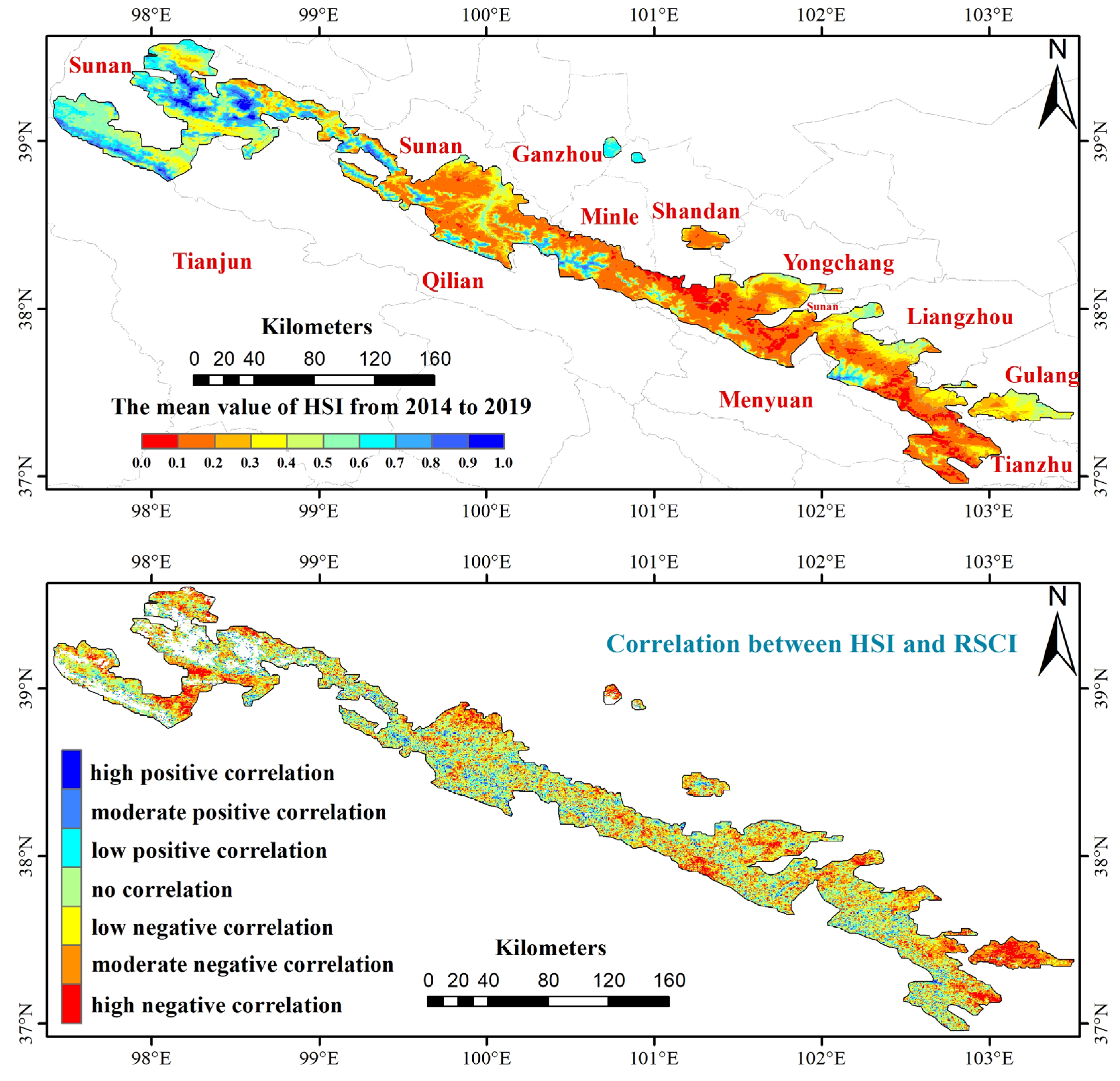
3.2.1. Analysis of Temporal and Spatial Correlation between Ecological Indicators and Human Activities

The HSI from 2014 to 2019 was calculated using the Nighttime Light (NTL) and Normalized Difference Vegetation Index (NDVI) data, and the spatial distribution of HSI showed an opposite trend to that of RSCI (Figure 8).Taking the analysis results with 90% confidence as an example, the Pearson correlation coefficient results in Figure 6 show that the human activity index negatively correlated with the ecological environment in 89.24% of the pixels (high negative correlation 55.18%, moderate negative correlation 34.06%), concentrated in Liangzhou District and Gulang County in the southeast. Those with a positive correlation accounted for only 10.76% (high negative correlation 5.66%, moderate positive correlation 5.09%) and had no specific spatial distribution(Figure 8).

RSCI and HSI from 2014 to 2019 showed a pronounced negative correlation trend; the values were mainly above 0.7 (RSCI) and below 0.2 (HSI). The maximum correlation coefficient appeared in 2019 (−0.825), followed by 2014 (−0.823) and 2017 (−0.812). This means that the overall environmental level of the study area is highly susceptible to the impact of human activities; the lower the intensity of human activities, the higher the ecological environment level (Figure 9 and Figure 10).

On a time scale, the intensity of human activities slowly declined from 2014 to 2019, consistent with the population density trend interpolated using government statistical data. Combined with the rising volatility in the RSCI index, the recovery in the ecological environment can be interpreted as the result of reducing destructive human activities.

The results of further analyses of the correlation between HSI and the eight ecological sub-indexes for RSCI are presented in Figure 11 and

Table 3. Sub-index pixel number statistics of maximum correlation.

Sub-Index	Number of Pixels	Proportion of Pixels
Qop/Qtco2	13,142	17.73%
EVI	12,372	16.69%
WET	9512	12.83%
NDBSI	9031	12.18%
AOD	8714	11.76%
LST	8040	10.85%
CRC	7437	10.03%
AI	5879	7.93%

. The ecological factors significantly affected by HSI were mainly carbon fixation and oxygen release, vegetation, and humidity; those less affected included surface temperature, climate, and landscape factors. The pixels highly correlated with carbon and oxygen release were evenly distributed. Those that were highly correlated with vegetation or humidity can be found mainly distributed in the Sunan Autonomous Region in the north and Gulang County in the southeast (also the main concentration area of highly negatively correlated pixels). The results illustrate how human activities affect the ecological environment in the Qilian Mountain Reserve.

On a spatial scale, the results of analyzing the spatial heterogeneity of human activities and ecological indicators by optimal parameters-based geographical detector (OPGD) are presented in Figure 10 [49]. The OPGD model puts forward the Q_v index to measure the interpretation degree of the spatial distribution of independent variables to dependent variables. The calculation formula of Q_v is:

$$Q_v=1-\frac{{\displaystyle {\sum }_{i=1}^M\left(N_{v,i}-1\right){\sigma }_{v,i}^2}}{\left(N_v-1\right){\sigma }_v^2}\times 100\%$$

(18)

where $N_v$ and ${\sigma }_v^2$ are the number and variance of the eight ecological sub-indexes or RSCI in the whole study area. $N_{v,i}$ and ${\sigma }_{v,i}^2$ are the number and variance in the ith sub-region of variable HSI or PD. The closer the Q_v value is to 100%, the more HSI or PD explains the spatial distribution of ecological sub-index or RSCI.

By running OPGD model with R programming language, the results show that the spatial interpretation degree of HSI for RSCI was 76.75%, while the spatial interpretation degree of PD for RSCI was only 9.67%. Qop/Qtco₂ (86.09%), EVI (85.45%) and NDBSI (83.86%) were significantly affected by the spatial distribution of HSI, while AI (6.92%) was least affected by HSI, which was highly consistent with the conclusion of correlation analysis. AOD (16.33%), LST (14.76%), and WET (14.10%) were significantly affected by PD spatial distribution. The Q_v value of PD was significantly lower than that of HSI. All the above results have passed the non-central F-distribution test (sig < 0.05). In addition, the OPGD model is used to calculate ecological detector (F-statistic) between ecological sub-indicators/RSCI and HSI/PD, so as to determine whether two independent variables have significantly different degrees of influence on the same dependent variable. The calculation formula of F-statistic is:

$$F=\frac{N_u\left(N_v-1\right){\displaystyle {\sum }_{j=1}^{M_u}{N}_{u,j}{\sigma }_{u,j}^2}}{N_v\left(N_u-1\right){\displaystyle {\sum }_{j=1}^{M_v}{N}_{v,j}{\sigma }_{v,j}^2}}$$

(19)

where the meaning represented by the mathematical symbols in the formula is basically the same as that in Formula (20). And the ecological detector results of OPGD model show that HSI has a higher significant influence than PD in the spatial distribution of all the sub-indicators and RSCI.

3.2.2. Human Activity-Ecological Environment Coupling State Classification Based on MK Test and Correlation Analysis

The correlation between RSCI and HSI and the Mann–Kendall test results for RSCI were used to cluster the impact of human activities on ecological conditions into different regions (Figure 12).

From 2014 to 2019, more than half of the regions exhibited a significant increase in RSCI. There was a negative correlation between HSI and RSCI, indicating the reduction in human-induced damage to the local environment and some ecological restoration from proper planning of anthropogenic activities. In addition, the HSI and RSCI increased synchronously in more than 10% of the regions, indicating that human activities and the local ecological environment were in a good state of coordinated evolution. In more than 30% of the region, the ecological changes were not caused by human activities, and in less than 1% was environmental deterioration due mainly to intensified human activities (

Table 4. Pixel reclassification based on the correlation analysis and the Mann–Kendall test.

Pixel Value	MK Test Result	Pearson Correlation Coefficient	Proportion of Pixels	Interpretation
0	NAN	NAN	NAN	Countless values or failed M-K test
1	Significant Increase	Negative correlation	56.61%	The decline of destructive human activities mitigated the deterioration of ecological conditions
2		No significant	31.23%	Human activities have little effect on the improvement of local environmental conditions
3		Positive correlation	10.35%	Human activities and local ecological environment promote each other
4	Significant Decline	Negative correlation	0.39%	Human destruction has aggravated the deterioration of the ecological environment
5		No significant	0.75%	Human activities have little effect on the deterioration of local environmental conditions
6		Positive correlation	0.67%	Affected by environmental degradation, the degree of livability decreases, leading to a decrease in human activities

).

3.2.3. Evaluation of Services Provided by Ecological Environment to Human Beings

Forty-one districts and counties around the study area were selected for further evaluation. Using published census data, the population density was interpolated and used in assessing the residents’ ESAI.

The ESAI spatial distribution (Figure 13) was different from RSCI. The region with the highest ESAI was concentrated in the middle of the study area, while people in northwest and southeast areas had relatively low ESAI. The values for RSCI, ESAI, and PD show that, while the population density in protected areas initially increased and then decreased, the average ESAI data at the three time points had a gradual increase for both walking range (3 km) and transportation range (10 km); the cumulative increase of ESAI in the 10 km range was close to 7.5%. This means that the rise in local population density did not reduce the residents’ per capita ecological welfare level, indicating a stable reciprocal relationship between human activities and the ecological environment in the study area. In addition, the declining trend of PD after 2010 was consistent with the changing trend of HSI, which confirmed the declining trend of human activities during this period.

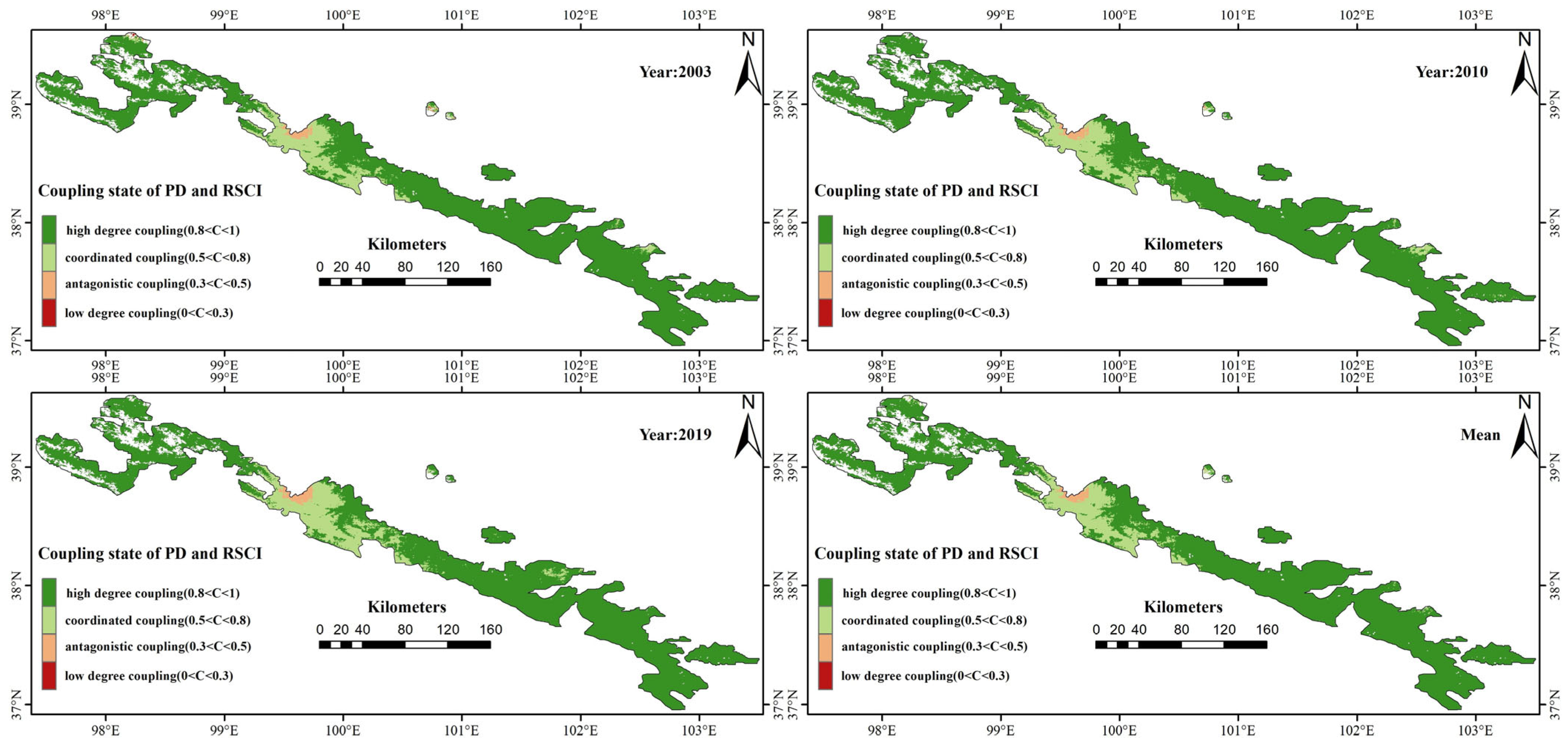
3.2.4. Analysis of Coupling Degree between Human Activity and Ecological Environment

The coupling degree results of RSCI and PD (Figure 14) also confirm a harmonious relationship between human activities and the ecological environment. The average coupling degree was above 0.9, with most areas in a state of coordinated coupling (C > 0.8). This suggests that human activities and the ecological environment influence each other, and that mutualism occurs.

The C value in most areas was above 0.6, which is in a medium–high coupling state. This is consistent with the results of the MK test and correlation analysis. Within the 10% confidence interval, more than 91.5% of the RSCI mutation areas showed a significant increase in ecological level and a decrease in the intensity of human activities; 89.9% of the areas had a high coupling degree (mean C value greater than 0.8). This confirms the rationality of the analysis method (Figure 15).

3.2.5. Analysis of Coupling State between Human Activity and Ecological Environment Based on Various Analysis Results

Based on the results of RSCI, MK test, correlation analysis, coupling degree analysis, and two-step floating catchment area method, the Human–Environment Composite Coupling Index (HECCI) was used to quantify the coupling effect between human activities and ecological environment in a specific region. The formula for calculating HECCI is

$$HECCI=\left(\alpha MK{C}_{ceo}+\beta C_{mean}\right)RSC{I}_{mean}+\gamma ESA{I}_{mean}$$

(20)

$$MK{C}_{ceo}=\frac{MK{C}_{pos}-MK{C}_{neg}}{MK{C}_{posall}-MK{C}_{negall}}$$

(21)

where $RSC{I}_{mean}$ is the average normalized RSCI of the area; $MK{C}_{pos}$ is the pixel proportion of the MK test and correlation analysis of the site (either 1 or 3); $MK{C}_{neg}$ is the pixel proportion of the MK test and correlation analysis of the area (either 4 or 6). $MK{C}_{posall}$ is the $MK{C}_{neg}$ for the entire study area; C is the average coupling degree; $ESA{I}_{mean}$ is the average ESAI index of the area; $\alpha$, $\beta$, $\gamma$ are the corresponding weight coefficients. In this study, $MK{C}_{posall}$ is 66.96%, $MK{C}_{negall}$ is 1.06%, and $\alpha$, $\beta$, $\gamma$ are 0.33.

After calculating the HECCI for each district and county, the results show that the regions with high human–environment coupling effects were mainly concentrated in autonomous prefectures (e.g., Sunan Autonomous Prefecture and Tianzhu Autonomous Prefecture) with HECCI above 0.4. The HECCI for Liangzhou District and Ganzhou District, with relatively developed economies and concentrated population densities, was low, only 0.299 and 0.221, respectively. This result also confirms the accuracy of the HECCI index in quantifying the coupling effect between human activities and the ecological environment. In particular, Ganzhou District had the lowest coupling degree in the study area. This means that the district should focus more on the coordinated development of its population and the ecological environment (Figure 16).

For Gulang County, although its comprehensive ecological level was in a very low sequence, its HECCI index increased to 0.341. The MK test results show that Gulang County’s ecological environment improved considerably in 2017 and 2019. Coincidentally, the local government vigorously promoted environmental protection starting in 2017. A higher $MK{C}_{ceo}$ in Gulang County means that human activities have a strong positive effect on the county’s environment. The results suggest that local environmental management should be encouraged, supported, and improved, particularly in areas with low ecological levels.

4. Discussion

The mechanisms by which human activities impact the ecological environment are highly complex, and factors influencing the ecological environment level are multifaceted. Previous studies on ecological environment assessment based on remote sensing data often focused on factors related to habitat quality. However, in this study, we have introduced a novel approach by integrating factors from three dimensions: habitat quality, landscape pattern and ecological services. Based on MODIS land cover imagery, the RSCI data from 2003 to 2019 were classified by different land cover types and organized into a box plot (Figure 17a). Regions with better ecological environments, such as forested areas, had higher RSCI values, with an average of 0.48. Conversely, regions with poorer ecological environments, such as bare land and built-up areas, had lower RSCI values, with average values of −0.17 and −0.09, respectively. This validates the rationality of the RSCI. The upward trend of RSCI between 2003 and 2019 is generally consistent with the facts of field research or the analysis results of other studies [50,51,52,53,54].

Meanwhile, based on the VIS and VISA frameworks [17,40], the remote-sensing-based ecological index (RSEI) and remote sensing model of UA eco-environment (RSUAE) were calculated for the period of 2003–2019, and classified using the same method (Figure 17b,c). The discriminatory ability of RSEI and RSUAE among different land cover types is basically consistent with that of RSCI, but RSCI contains more useful environmental information such as landscape pattern and ecological services, making it more advantageous in terms of information content.

The commonly used indicators of coupling degree and coupling coordination degree cannot fully quantify the coupling relationship between human activities and the ecological environment [23,24,25]. Therefore, concepts such as MK-correlation classification and ESAI are introduced to describe the interaction between human activities and the ecological environment from multiple angles.

Since its establishment in 1986, the Qilian Mountain Nature Reserve has experienced serious ecological damage. In response, the Chinese government has introduced various targeted policies to support the ecological restoration and reconstruction of the protected area. Based on our analysis of its ecological environment from 2003 to 2019, the RSCI showed a gradually increasing trend. The improvements in the environmental status of the Qilian Mountain Nature Reserve are related not only to natural factors (e.g., climate) but also anthropogenic parameters, such as vegetation cover, infrastructure, carbon emissions, and air quality (Figure 4 and Figure 10b) [55].

The spatial distribution of the RSCI reveals that the ecological environment level in Gulang County, Liangzhou District and the northwest region of Sunan is relatively low (Figure 5). The correlation analysis between the eight ecological sub-indices and HSI also indicates a strong negative correlation between the human-influenced indicators (such as EVI) and human activities in these three areas (Figure 11). This suggests a close relationship between local human activities and the ecological environment in these regions. However, it is worth noting that, unlike Gulang County and Liangzhou District, the MK test results indicate that the magnitude of change in RSCI in the Sunan region during the period from 2003 to 2019 is not significantly pronounced compared to the other two regions (Figure 6).

Due to its higher altitude, cold temperatures, and sparse population, the ecological level in the Sunan region is primarily influenced by external environmental conditions such as climate. While the results of C indicate a relatively good human activities–ecological environment coupling status in Sunan, achieving significant improvements in the ecological environment through rational planning of human activities is challenging due to the area’s adverse natural conditions and sparse human population.

In contrast, Gulang County and Liangzhou District have higher population densities and greater urbanization levels. As a result, the local ecological environment exhibits a higher degree of response to government policies restricting human activities and promoting environmental restoration. The year of significant change in RSCI also coincides with the year of policy implementation (Figure 7). The positive effect of relevant government policies on the ecological environment of the study area has also been unanimously recognized by other studies [56].

By employing various methods for comprehensive analysis and comparison, it is possible not only to differentiate the degree to which different regions are affected by human activities on the ecological environment but also to delve into the driving forces behind ecological changes. Moreover, these approaches allow for a certain degree of quantification in assessing the feasibility of implementing measures that can restrict human activities to improve the local ecological environment.

Whether from the correlation coefficient between HSI and RSCI or from the years when RSCI increased significantly, the human impact on the study area’s comprehensive environmental status has improved considerably since 2017. From January 2017 to August 2019, various measures and efforts tackling the ecological problems of the Qilian Mountain National Nature Reserve were provided by the Chinese Government to promote conservation and environmental programs in Gulang, Tianzhu, Sunan, and other places. As supported by the study’s findings, environmental protection decisions by the local government can effectively restrain the destructive effects of human activities and help restore the ecological environment.

During the period from 2003 to 2010, there was a significant increase (3.57%) in population density in the study area. However, both the RSCI and the ESAI did not exhibit a decrease in 2010; instead, they showed slight improvements (Figure 5, Figure 13 and Figure 15). From 2010 to 2019, the HSI and PD indices, representing human activity levels, consistently declined annually, while the RSCI and ESAI, representing ecological environment levels, demonstrated an upward trend. Moreover, the increase in RSCI and ESAI during this period was more substantial compared to the 2003–2010 period. For instance, the 10 km ESAI reflected an increase in per capita ecological welfare level from 0.609 in 2003–2010 to 0.620, and further rose to 0.656 in 2010–2019. These findings suggest that although an increase in human population and activity levels can potentially have negative impacts on ecological environment changes, it does not necessarily result in a decline in ecological environment levels. By effectively regulating local human activities and enhancing the coupling between human activities and the ecological environment (C), it becomes feasible to mitigate the adverse effects of human activities on the ecological environment to some extent (Figure 15 and Figure 16). The results of this study should be interpreted with caution in light of some shortcomings. For example, the resolution of the RSCI was limited, which could have influenced the results. Subsequent studies should consider using higher-resolution images and advanced remote sensing techniques to improve the RSCI resolution. Compared to other environmental indices, RSCI incorporates a greater amount of ecological environment information. However, the inclusion of more input data also implies increased uncertainty, which inevitably has a higher impact on the accuracy of the analysis results. Human activities were considered homogenous and were not properly contextualized. Given the heterogeneity of anthropogenic activities and their varying impact on the ecological environment, future studies can look into using categories or clusters of human activities for better differentiation and more nuanced analyses.

5. Conclusions

The ecological environment of the Qilian Mountains Nature Reserve was evaluated systematically and comprehensively through an ecological evaluation method that integrated environmental quality, landscape patterns, and ecological service functions. The MK test and correlation analysis were combined to evaluate and analyze the coupling between human activities and the local environment. Through comparison and integration with other methods, the human–environment coupling process in Qilian Mountain Nature Reserve was analyzed from multiple perspectives. The rationality of the proposed assessment method was verified, providing new insights into human activity–ecological environment coupling and interactions. The main conclusions are as follows:

1.

Evaluation of comprehensive ecological conditions

The ecological environment of Qilian Mountain Nature Reserve is gradually recovering due to improvements in the natural conditions, the three North shelterbelts, and other human environmental policies [57]. Since 2003, temperature, humidity, and atmospheric conditions have become more suitable for vegetation, and the comprehensive environmental level (RSCI) has increased annually, from 0.513 in 2004 to 0.649 in 2017.

2.

Correlation and spatial heterogeneity between human activities and the environment

Data from 2000, 2010, and 2020 censuses show that the average population density in the Qilian Mountain Nature Reserve increased first and then decreased since 2003. During 2014–2019, the human activity index (HSI) also exhibited a downward annual trend. The correlation analysis between HSI and RSCI suggests that the intensity of human activity had a pronounced negative correlation with the comprehensive ecological level; the correlation coefficient reached −0.825 in 2019. The main ecological sub-indexes greatly affected by human activities were carbon fixation and oxygen release (Qop/Qtco₂), vegetation (EVI), and humidity (WET); their pixel proportions were 17.73%, 16.69%, and 12.83%, respectively. The ecological sub-indexes that were greatly influenced by HSI space were carbon fixation and oxygen release (Qop/Qtco₂), vegetation (EVI), and soil (NDBSI); their spatial interpretation degrees were 86.09%, 85.45%, and 83.86%, respectively. Compared with population interpolation data, remote sensing human activity index has a significant advantage in the degree of influence on the spatial distribution of ecological environment.

3.

Human–environment coupling evaluation based on MK test and correlation analysis

Using the results from the MK test and correlation analysis, the man–environment coupling state was divided spatially. From 2014 to 2019, more than 56% of the Qilian Mountain Nature Reserve recovered ecologically due to decreased human activities, while less than 1% of the areas experienced environmental deterioration from intensified human activities. Most pixels had mutation years in 2017 and 2019, mainly concentrated in Gulang County, Tianzhu Autonomous Region, and Yongchang County. The results could be related to the vigorous implementation of some environmental policies by the Chinese government during 2017–2019.

4.

Comparison and fusion of coupling analysis and accessibility analysis

The coupling analysis between population density and the RSCI index for 2003–2019 suggests that the human–environment system in most parts of the study area was medium to high coupling, consistent with the results of the MK test and correlation analysis. The continuous growth in ESAI indicates that the ecological welfare per capita has gradually increased. Overall, the increase in human activity intensity did not exceed the recovery rate of the ecological environment. The results of the MK test, correlation coefficients, ecological accessibility, and coupling degree of the human–natural system all suggest that the local population and ecosystem in the Qilian Mountains are in collaborative development.

Combining the results of the three methods, a new index (HECCI) is proposed to evaluate the comprehensive human–environment coupling level at the regional scale. The HECCI of 11 districts and counties in the Qilian Mountain Nature Reserve was analyzed. The results show that the human–environment comprehensive coupling degree was higher in Sunan and Tianzhu autonomous regions, with HECCI values above 0.4. In the economically developed Liangzhou District and Ganzhou District, the HECCI values were extremely low, which could be related to their fragile ecological environments. However, Gulang County, which also has a fragile ecological environment, was found to have a high HECCI value (0.341). One possible reason for how Gulang County bucked the trend could be the environmental management policies that have been implemented in the county since 2017.

References

1. Aslan, A.; Altinoz, B.; Ozsolak, B. The link between urbanization and air pollution in Turkey: Evidence from dynamic autoregressive distributed lag simulations. Environ. Sci. Pollut. Res. 2017, 28, 52370–52380. [Google Scholar] [CrossRef] [PubMed]
2. Kolpin, D.; Furlong, E.; Meyer, M.; Thurman, E.; Zaugg, S.; Barber, L.; Buxton, H. Pharmaceuticals, hormones, and other organic wastewater contaminants in US streams, 1999–2000: A national reconnaissance. Environ. Sci. Technol. 2002, 36, 1202–1211. [Google Scholar] [CrossRef] [PubMed] [Green Version]
3. Nriagu, J.O.; Pacyna, J.M. Quantitative assessment of worldwide contamination of air, water and soils by trace metals. Nature 1998, 333, 134–139. [Google Scholar] [CrossRef] [PubMed]
4. Ni, J.L.; Cai, L.; Wang, J.K. Application Research on the Coupled Human-Environment Ecosystem Vulnerability Assessment in Different Spatial and Temporal Scales. Appl. Mech. Mater. 2014, 535, 255–265. [Google Scholar] [CrossRef]
5. Gurney, K.R.; Romero-Lankao, P.; Seto, K.C.; Hutyra, L.R.; Duren, R.; Kennedy, C.; Grimm, N.B.; Ehleringer, J.R.; Marcotullio, P.; Hughes, S.; et al. Climate change track urban emissions on a human scale. Nature 2015, 525, 179–181. [Google Scholar] [CrossRef] [Green Version]
6. Wang, S.; Fu, B.; Zhao, W.; Liu, Y.; Wei, F. Structure, function, and dynamic mechanisms of coupled human–natural systems. Curr. Opin. Environ. Sustain. 2018, 33, 87–91. [Google Scholar] [CrossRef]
7. Koutsoyiannis, D.; Kundzewicz, Z.W. Atmospheric Temperature and CO2: Hen-Or-Egg Causality? Science 2020, 2, 83. [Google Scholar] [CrossRef]
8. Coppin, P.; Jonckheere, I.; Nackaerts, K.; Muys, B.; Lambin, E. Digital change detection methods in ecosystem monitoring: A review. Int. J. Remote Sens. 2004, 25, 1565–1596. [Google Scholar] [CrossRef]
9. Song, W.; Song, W.; Gu, H.; Li, F. Progress in the Remote Sensing Monitoring of the Ecological Environment in Mining Areas. Int. J. Environ. Res. Public Health 2020, 17, 1846. [Google Scholar] [CrossRef] [Green Version]
10. Zhao, J.; Wang, J.; Hong, Q.; Song, Q.; Huang, L.; Zhang, D. Investigation of Natural Ecological Enviroment Using Remote Sensing Based Integrated Index at A City Scale. In Proceedings of the IGARSS 2018—2018 IEEE International Geoscience and Remote Sensing Symposium, Valencia, Spain, 22–27 July 2018; pp. 2467–2470. [Google Scholar]
11. Liu, J.; Dietz, T.; Carpenter, S.R.; Folke, C.; Alberti, M.; Redman, C.L.; Schneider, S.H.; Ostrom, E.; Pell, A.N.; Lubchenco, J.; et al. Coupled human and natural systems. Ambio 2007, 36, 639–649. [Google Scholar] [CrossRef]
12. Liu, H.; Fang, C.; Fang, K. Coupled Human and Natural Cube: A novel framework for analyzing the multiple interactions between humans and nature. J. Geogr. Sci. 2020, 30, 355–377. [Google Scholar] [CrossRef]
13. Handfield, R.; Walton, S.V.; Sroufe, R.; Melnyk, S.A. Applying environmental criteria to supplier assessment: A study in the application of the Analytical Hierarchy Process. Eur. J. Oper. Res. 2002, 141, 70–87. [Google Scholar] [CrossRef]
14. Wang, X.; Cao, Y.; Zhong, X.; Gao, P. A new method of regional eco-environmental quality assessment and its application. J. Environ. Qual. 2012, 41, 1393–1401. [Google Scholar] [CrossRef] [PubMed] [Green Version]
15. Hu, X.; Xu, H. A new remote sensing index based on the pressure-state-response framework to assess regional ecological change. Env. Sci. Pollut. Res. Int. 2019, 26, 5381–5393. [Google Scholar] [CrossRef]
16. Tian, X.; Ju, M.; Shao, C.; Fang, Z. Developing a new grey dynamic modeling system for evaluation of biology and pollution indicators of the marine environment in coastal areas. Ocean Coast. Manag. 2011, 54, 750–759. [Google Scholar] [CrossRef]
17. Kosiba, P. Self-organizing feature maps and selected conventional numerical. Acta Soc. Bot. Pol. 2009, 78, 335–343. [Google Scholar] [CrossRef]
18. Xu, H.; Wang, Y.; Guan, H.; Shi, T.; Hu, X. Detecting Ecological Changes with a Remote Sensing Based Ecological Index (RSEI) Produced Time Series and Change Vector Analysis. Remote Sens. 2019, 11, 2345. [Google Scholar] [CrossRef] [Green Version]
19. Liu, W.; Chen, G. Evolution of Ecosystem Service Value and Ecological Storage Estimation in Huainan Coal Mining Area. Bull. Env. Contam. Toxicol. 2021, 107, 1243–1249. [Google Scholar] [CrossRef]
20. Liu, Y.; Li, J.; Xia, J.; Hao, G.; Teo, F. Risk assessment of non-point source pollution based on landscape pattern in the Hanjiang River basin, China. Env. Sci. Pollut. Res. Int. 2021, 28, 64322–64336. [Google Scholar] [CrossRef]
21. Costanza, R.; d’Arge, R.; Groot, R.d.; Farber, S.; Grasso, M.; Hannon, B.; Limburg, K.; Naeem, S.; O’Neill, R.V.; Paruelo, J.; et al. The value of the world’s ecosystem services and natural capital. Nature 1997, 387, 253–260. [Google Scholar] [CrossRef]
22. Hu, X.; Xu, H. A new remote sensing index for assessing the spatial heterogeneity in urban ecological quality: A case from Fuzhou City, China. Ecol. Indic. 2018, 89, 11–21. [Google Scholar] [CrossRef]
23. Sanze, F.; Huimin, Z.; Hui, S.; Jianchun, W.; Lijun, R. Examination of a coupling coordination relationship between urbanization and the eco-environment: A case study in Qingdao, China. Env. Sci. Pollut. Res. Int. 2020, 27, 23981–23993. [Google Scholar] [CrossRef]
24. Huang, M.; Li, Y.; Xia, C.; Zeng, C.; Zhang, B. Coupling responses of landscape pattern to human activity and their drivers in the hinterland of Three Gorges Reservoir Area. Glob. Ecol. Conserv. 2022, 33, e01992. [Google Scholar] [CrossRef]
25. Zhang, X.; Xu, Z. Functional Coupling Degree and Human Activity Intensity of Production–Living–Ecological Space in Underdeveloped Regions in China: Case Study of Guizhou Province. Land 2021, 10, 56. [Google Scholar] [CrossRef]
26. Chai, L.H.; Lha, D. A new approach of deriving indicators and comprehensive measure for ecological environmental quality assessment. Ecol. Indic. 2018, 85, 716–728. [Google Scholar] [CrossRef]
27. Ji, Z.; Yingjie, H.; Boldanov, T.; Bazarzhapov, T.; Dan, M.; Li, Y.; Dong, S. Comprehensive assessment of the coupling coordination degree between urbanization and ecological environment in the Siberian and Far East Federal Districts, Russia from 2005 to 2017. PeerJ 2020, 8, e9125. [Google Scholar] [CrossRef]
28. Liu, J.; Dietz, T.; Carpenter, S.R.; Albert, M.; Folk, C.; Moran, E.; Pell, A.N.; Deadman, P.; Kratz, T.; Lubchenc, J.; et al. Complexity of coupled human and natural systems. Science 2007, 317, 1513–1516. [Google Scholar] [CrossRef] [Green Version]
29. Ostrom, E. A general framework for analyzing sustainability of social-ecological systems. Science 2009, 325, 419–422. [Google Scholar] [CrossRef]
30. Liu, J.; Hull, V.; Godfray, H.C.J.; Tilman, D.; Gleick, P.; Hoff, H.; Pahl-Wostl, C.; Xu, Z.; Chung, M.G.; Sun, J.; et al. Nexus approaches to global sustainable development. Nat. Sustain. 2018, 1, 466–476. [Google Scholar] [CrossRef]
31. Holling, C. Understanding the Complexity of Economic, Ecological, and Social Systems. Ecosystems 2001, 4, 390–405. [Google Scholar] [CrossRef]
32. Firozjaei, M.K.; Fathololoumi, S.; Weng, Q.; Kiavarz, M.; Alavipanah, S.K. Remotely Sensed Urban Surface Ecological Index (RSUSEI): An Analytical Framework for Assessing the Surface Ecological Status in Urban Environments. Remote Sens. 2020, 12, 2029. [Google Scholar] [CrossRef]
33. Ma, H.; Shi, L. Assessment of eco-environmental quality of Western Taiwan Straits Economic Zone. Environ. Monit. Assess. 2016, 188, 311–321. [Google Scholar] [CrossRef] [PubMed]
34. Reza, M.I.H.; Abdullah, S.A. Regional Index of Ecological Integrity: A need for sustainable management of natural resources. Ecol. Indic. 2011, 11, 220–229. [Google Scholar] [CrossRef]
35. Wei, W.; Guo, Z.; Xie, B.; Zhou, J.; Li, C. Spatiotemporal evolution of environment based on integrated remote sensing indexes in arid inland river basin in Northwest China. Env. Sci. Pollut. Res. Int. 2019, 26, 13062–13084. [Google Scholar] [CrossRef] [PubMed]
36. Xu, H.; Wang, M.; Shi, T.; Guan, H.; Fang, C.; Lin, Z. Prediction of ecological effects of potential population and impervious surface increases using a remote sensing based ecological index (RSEI). Ecol. Indic. 2018, 93, 730–740. [Google Scholar] [CrossRef]
37. Boumans, R.; Roman, J.; Altman, I.; Kaufman, L. The Multiscale Integrated Model of Ecosystem Services (MIMES): Simulating the interactions of coupled human and natural systems. Ecosyst. Serv. 2015, 12, 30–41. [Google Scholar] [CrossRef]
38. Yan, K.; Ding, Y. The overview of the progress of Qilian Mountain National Park System Pilot Area. Int. J. Geoheritage Parks 2020, 8, 210–214. [Google Scholar] [CrossRef]
39. Zhang, Q.; Schaaf, C.; Seto, K.C. The Vegetation Adjusted NTL Urban Index: A new approach to reduce saturation and increase variation in nighttime luminosity. Remote Sens. Environ. 2013, 129, 32–41. [Google Scholar] [CrossRef]
40. Luo, W. Using a GIS-based floating catchment method to assess areas with shortage of physicians. Health Place 2004, 10, 1–11. [Google Scholar] [CrossRef]
41. Sun, H.; Wu, L.; Hu, J.; Ma, L.; Li, H.; Wu, D. Evaluating eco-environment in urban agglomeration from a vegetation-impervious surface-soil-air framework: An example in Ningxia, China. J. Appl. Remote Sens. 2021, 15, 014518. [Google Scholar] [CrossRef]
42. Jimenez-Munoz, J.C.; Sobrino, J.A.; Skokovic, D.; Mattar, C.; Cristobal, J. Land Surface Temperature Retrieval Methods From Landsat-8 Thermal Infrared Sensor Data. IEEE Geosci. Remote Sens. Lett. 2014, 11, 1840–1843. [Google Scholar] [CrossRef]
43. Peng, J.; Wang, Y.; Zhang, Y.; Wu, J.; Li, W.; Li, Y. Evaluating the effectiveness of landscape metrics in quantifying spatial patterns. Ecol. Indic. 2010, 10, 217–223. [Google Scholar] [CrossRef]
44. He, H.S.; DeZonia, B.E.; Mladenoff, D.J. An aggregation index (AI) to quantify spatial patterns of landscapes. Landsc. Ecol. 2000, 15, 591–601. [Google Scholar] [CrossRef]
45. Yue, S.; Pilon, P.; Cavadias, G. Power of the Mann-Kendall and Spearman’s rho tests for detecting monotonic trends in hydrological series. J. Hydrol. 2002, 259, 254–271. [Google Scholar] [CrossRef]
46. Koo, T.K.; Li, M.Y. A Guideline of Selecting and Reporting Intraclass Correlation Coefficients for Reliability Research. J. Chiropr. Med. 2016, 15, 155–163. [Google Scholar] [CrossRef] [PubMed] [Green Version]
47. Nelson, E.; Mendoza, G.; Regetz, J.; Polasky, S.; Tallis, H.; Cameron, D.; Chan, K.M.A.; Daily, G.C.; Goldstein, J.; Kareiva, P.M.; et al. Modeling multiple ecosystem services, biodiversity conservation, commodity production, and tradeoffs at landscape scales. Front. Ecol. Environ. 2009, 7, 4–11. [Google Scholar] [CrossRef]
48. Abdullah, S.; Adnan, M.S.G.; Barua, D.; Murshed, M.M.; Kabir, Z.; Chowdhury, M.B.H.; Hassan, Q.K.; Dewan, A. Urban green and blue space changes: A spatiotemporal evaluation of impacts on ecosystem service value in Bangladesh. Ecol. Inform. 2022, 70, 101730. [Google Scholar] [CrossRef]
49. Song, Y.; Wang, J.; Ge, Y.; Xu, C. An optimal parameters-based geographical detector model enhances geographic characteristics of explanatory variables for spatial heterogeneity analysis: Cases with different types of spatial data. GISci. Remote Sens. 2020, 57, 593–610. [Google Scholar] [CrossRef]
50. Xue, J.; Li, Z.; Feng, Q.; Li, Z.; Gui, J.; Li, Y. Ecological conservation pattern based on ecosystem services in the Qilian Mountains, northwest China. Environ. Dev. 2023, 46, 100834. [Google Scholar] [CrossRef]
51. Liu, Y.; Liu, X.; Zhao, C.; Wang, H.; Zang, F. The trade-offs and synergies of the ecological-production-living functions of grassland in the Qilian mountains by ecological priority. J. Environ. Manag. 2023, 327, 116883. [Google Scholar] [CrossRef]
52. Shan, S.Y.; Xu, H.J.; Qi, X.L.; Chen, T.; Wang, X.D. Evaluation and prediction of ecological carrying capacity in the Qilian Mountain National Park, China. J. Env. Manag. 2023, 339, 117856. [Google Scholar] [CrossRef] [PubMed]
53. Wang, H.; Liu, C.; Zang, F.; Liu, Y.; Chang, Y.; Huang, G.; Fu, G.; Zhao, C.; Liu, X. Remote Sensing-Based Approach for the Assessing of Ecological Environmental Quality Variations Using Google Earth Engine: A Case Study in the Qilian Mountains, Northwest China. Remote Sens. 2023, 15, 960. [Google Scholar] [CrossRef]
54. Wang, Y.; Zhao, R.; Li, Y.; Yao, R.; Wu, R.; Li, W. Research on the evolution and the driving forces of land use classification for production, living, and ecological space in China’s Qilian Mountains Nature Reserve from 2000 to 2020. Env. Sci. Pollut. Res. Int. 2023, 30, 64949–64970. [Google Scholar] [CrossRef] [PubMed]
55. Peng, Q.; Wang, R.; Jiang, Y.; Li, C. Contributions of climate change and human activities to vegetation dynamics in Qilian Mountain National Park, northwest China. Glob. Ecol. Conserv. 2021, 32, e01947. [Google Scholar] [CrossRef]
56. Zongxing, L.; Qi, F.; Zongjie, L.; Xufeng, W.; Juan, G.; Baijuan, Z.; Yuchen, L.; Xiaohong, D.; Jian, X.; Wende, G.; et al. Reversing conflict between humans and the environment—The experience in the Qilian Mountains. Renew. Sustain. Energy Rev. 2021, 148, 111333. [Google Scholar] [CrossRef]
57. Mu, H.; Li, X.; Ma, H.; Du, X.; Huang, J.; Su, W.; Yu, Z.; Xu, C.; Liu, H.; Yin, D.; et al. Evaluation of the policy-driven ecological network in the Three-North Shelterbelt region of China. Landsc. Urban Plan. 2022, 218, 104305. [Google Scholar] [CrossRef]
Figure 1. Research area survey. (a) NDVI image of study area; (b) Elevation image of study area.
Sustainability 15 11177 g001
Figure 2. Ecological sub-indicator images (take 2019 images as an example): (a) AOD; (b) EVI; (c) LST; (d) NDBSI; (e) WET; (f) AI; (g) CRC; (h) Qop/Qtco2.
Sustainability 15 11177 g002
Figure 3. Workflow diagram.
Sustainability 15 11177 g003
Figure 4. (a) The annual normalized values of the ecological evaluation sub-indexes; (b) The coefficient of sensitivity of the ecological evaluation sub-indexes; (c) The principal component weights of the ecological evaluation sub-indexes.
Sustainability 15 11177 g004
Figure 5. The spatial distribution and numerical changes of RSCI.
Sustainability 15 11177 g005
Figure 6. The result of the Mann–Kendall test.
Sustainability 15 11177 g006
Figure 7. MK mutation year.
Sustainability 15 11177 g007
Figure 8. The Pearson correlation coefficient results of HSI and RSCI.
Sustainability 15 11177 g008
Figure 9. Gaussian Kernel Density Distribution of HSI and RSCI (2014–2019).
Sustainability 15 11177 g009
Figure 10. (a) Mean value of RSCI and HSI and the correlation coefficient between them (2014–2019); (b) OPGD model results of PD and HSI.
Sustainability 15 11177 g010
Figure 11. The name of the sub-index with the largest absolute correlation with HSI and the correlation value (2014–2019).
Sustainability 15 11177 g011
Figure 12. Pixel reclassification based on correlation analysis and Mann–Kendall test.
Sustainability 15 11177 g012
Figure 13. The image of PD, ESAI (3 km) and ESAI (10 km) in 2003, 2010, and 2019.
Sustainability 15 11177 g013
Figure 14. The coupling degree of RSCI and PD in 2003, 2010 and 2019.
Sustainability 15 11177 g014
Figure 15. (a) ESAI violin drawing; (b) C violin drawing.
Sustainability 15 11177 g015
Figure 16. HECCI, RSCImean, Cmean, ESAImean, MKCceo, and area proportion statistics of each county.
Sustainability 15 11177 g016
Figure 17. Boxplots of RSCI (a), RSEI (b), and RSUAE (c) based on different land cover types.
Sustainability 15 11177 g017