Article

Temperature Prediction Based on STOA-SVR Rolling Adaptive Optimization Model

1
College of Mathematical Science, Yangzhou University, Siwangting Road 180, Yangzhou 225127, China
2
Glorious Sun School of Business and Management, Donghua University, West Yan’an Road 1882, Shanghai 200051, China
3
Maanshan Power Supply Company, Huayu Road 7, Maanshan 243000, China
4
School of Mechanical Engineering, Yangzhou University, Huayang West Road 196, Yangzhou 225127, China
*
Author to whom correspondence should be addressed.
Sustainability 2023, 15(14), 11068; https://doi.org/10.3390/su151411068
Submission received: 30 May 2023 / Revised: 10 July 2023 / Accepted: 12 July 2023 / Published: 15 July 2023

Abstract

:
In this paper, a support vector regression (SVR) adaptive optimization rolling composite model with a sooty tern optimization algorithm (STOA) has been proposed for temperature prediction. Firstly, aiming at the problem that the algorithm tends to fall into the local optimum, the model introduces an adaptive Gauss–Cauchy mutation operator to effectively increase the population diversity and search space and uses the improved algorithm to optimize the key parameters of the SVR model, so that the SVR model can mine the linear and nonlinear information in the data well. Secondly, the rolling prediction is integrated into the SVR prediction model, and the real-time update and self-regulation principles are used to continuously update the prediction, which greatly improves the prediction accuracy. Finally, the optimized STOA-SVR rolling forecast model is used to predict the final temperature. In this study, the global mean temperature data set from 1880 to 2022 is used for empirical analysis, and a comparative experiment is set up to verify the accuracy of the model. The results show that compared with the seasonal autoregressive integrated moving average (SARIMA), feedforward neural network (FNN) and unoptimized STOA-SVR-LSTM, the prediction performance of the proposed model is better, and the root mean square error is reduced by 6.33–29.62%. The mean relative error is reduced by 2.74–47.27%; the goodness of fit increases by 4.67–19.94%. Finally, the global mean temperature is predicted to increase by about 0.4976 °C in the next 20 years, with an increase rate of 3.43%. The model proposed in this paper not only has a good prediction accuracy, but also can provide an effective reference for the development and formulation of meteorological policies in the future.

1. Introduction

Meteorology plays a vital role in human production, life and health, and global temperature change has become one of the main indicators to measure meteorological change [1]. Since the industrial revolution, all countries have entered a period of rapid economic development, and the massive use of fossil energy is causing CO2 emissions to increase year by year. However, the resources that can absorb CO2, such as forests and wetlands, are being excessively destroyed, the energy absorbed and released by the Earth’s atmospheric system is becoming unbalanced and the greenhouse effect continues to accumulate, leading to a steady rise in global temperature [2]. Especially since the beginning of the 21st century, a large number of countries or regions have reported surprisingly high temperatures, and climate warming has become a major challenge for humanity [3]. In order to prevent the adverse effects of these extremely high temperatures on society in advance, it is necessary to unearth the hidden information in the existing historical temperature data and use this information to accurately predict the future temperature.
A temperature time series includes the interaction of many aspects, and the final result is non-linear and unstable, and the data are very random, making it difficult to predict accurately. However, refined temperature prediction results can not only guide people to arrange their work and daily life in an orderly manner, but also provide decision support for early warning of potential meteorological disasters, which is of great significance for national policy development and people’s lives [4,5]. Therefore, in recent years, more and more scholars have started to study temperature prediction and analyze the causes of global warming. Accurate temperature prediction and the study of the causes and influencing factors of temperature change have become the focus of scientific and social circles.
At present, most researchers focus on the application of various models for prediction. However, they lack further optimization of the model itself, and they often choose empirical values for some important super-parameters in machine learning, which may weaken the prediction accuracy. Second, most studies mainly use static data sources in the data matrix for prediction analysis. Since temperature prediction is a long-term data prediction, static data may lead to an increase in the final error, resulting in a decrease in the accuracy of the prediction results. To this end, this study has made improvements on the above points, and the main contributions are as follows:
(1)
The key parameters of the SVR model are optimized by using the sooty tern algorithm. Considering the problem that the sooty tern algorithm tends to fall into the local optimum, the model introduces the adaptive Gauss–Cauchy mutation operator to effectively increase the population diversity and search space.
(2)
This paper integrates the real-time updating and self-regulation principle based on rolling prediction into the SVR model, and it uses the updated data by eliminating the earliest data series so as to effectively improve the problem of accuracy decline caused by the long prediction cycle.
(3)
The SVR and long short-term memory (LSTM) models are applied to the research of temperature prediction. LSTM models can solve the problem that the traditional neural network model is unable to process the long time series to predict the residual error of SVR, so as to further improve the prediction accuracy.
The rest of the paper is organized as follows: Section 2 is a summary of the relevant literature from the two aspects of the single method prediction model and the combination method prediction model; Section 3 presents the sources of the data used in this study and pre-processes the collected global annual mean temperature data. Section 4 introduces the proposed optimization algorithm and a research model for long-term temperature prediction. In Section 5, the data set is divided into training and test sets, and the model proposed in this paper is used for empirical analysis. Section 6 compares the prediction performance of the proposed model with other typical advanced methods, discusses the validity and accuracy of the model, and predicts the data for the next 20 years. Section 7 summarizes the main results of this paper.

2. Related Works

In order to accurately predict the temperature, many scholars have conducted a lot of research; there are a lot of temperature prediction methods, including the establishment of a single model for forecasting and the establishment of a combination model for forecasting.

2.1. Predictive Model Based on a Single Method

The establishment of a prediction model based on a single method aimed mainly to use the original data set, mining the historical law of the data, and then use the model to continue the law, so as to make predictions. This prediction method mainly includes the mathematical statistics prediction method and the machine learning prediction method.
In terms of the mathematical statistical forecasting methods, Harnack et al. [6] used jackknifed regression and a measure of intra-seasonal atmospheric circulation variability to predict the pacific sea surface temperature (SST). By greatly increasing the effective independent sample size, the introduction of jackknifed regression makes the prediction technique more quantifiable than in previous studies. Zhang et al. [7] proposed a new multivariate gray prediction model considering the spatial proximity effect for time series prediction, constructed the spatial proximity effect term, incorporated it into the traditional discrete multivariate gray model and established a new model to overcome the problem of ignoring spatial features in the traditional gray model. The experimental results show that the proposed method is robust and can be widely applied. Liang [8] used the autoregressive integrated moving average (ARIMA) model to study the air temperature prediction in Antarctica and analyzed the factors affecting the surface air temperature in Antarctica. Saha et al. [9] developed a space-time autoregressive moving average (STARMA) model based on a fuzzy inference system (FIS) weight matrix, which accurately predicted the temperature of West Bengal in India. The proposed fuzzy rule-based weighted STARMA model was found to be superior to both the STARMA and ARIMA models. In the case of temperature forecasts, Möller et al. [10] proposed combining the state-of-the-art ensemble model output statistics (EMOS) with an ensemble adjusted by an autoregressive process fitted to the respective error series by a spread-adjusted linear pool to reduce the uncertainty in the outputs of numerical weather prediction (NWP) models. Motivated by the observation that adjacent regions usually show similar temperature trends, Shi et al. [11] considered temperature prediction as a spatiotemporal sequence prediction problem and proposed a new self-attention joint spatiotemporal network (SA-JSTN) deep learning model for temperature prediction which is able to integrate the global spatial correlation into the temperature series prediction problem, thus showing better performance especially in short-term prediction. Kim et al. [12] established hierarchical models with time-varying parameters by considering the coefficient and variance of the state-space model, discussed the Bayesian inference of such models and applied them to hemispheric surface temperature prediction.
For the machine learning forecasting method, Fister et al. [13] used three different computational frameworks for temperature forecasting: a convolutional neural network (CNN) with video-to-image translation, several ML approaches including lasso regression, decision trees and random forest, and finally a CNN with a preprocessing step using recurrence plots that convert time series into images. Using these frameworks, very good forecasting capabilities were obtained for the Paris and Cordoba regions. Joshi et al. [14] predicted the extreme temperature (maximum and minimum temperature) of the Himalayas in winter based on an artificial neural network (ANN), which has obvious advantages in the application of temperature prediction. Wei et al. [15] separated the SST time series data into climatological monthly mean and monthly anomaly data sets and constructed two ANN models. The combination of these two models provides the final SST prediction results. This method was applied to the 12-month lead time SST prediction in the South China Sea. The results show that the proposed training method provides good prediction accuracy. Haq et al. [16] used the LSTM model to predict the ambient temperature in Himachal Pradesh with data sets, and the result reflected that the LSTM performed better than the ANN in the time series verification of single parameters. Alomar et al. [17] used a variety of machine learning algorithms such as regression tree (RT), SVR, quantified regression tree (QRT), random forest (RF) and gradient lift regression (GBR) to predict short and medium term (daily and weekly) air temperatures over the North American continental climate. It was found that both RT and SVR performed very well in predicting weekly temperatures. Radhika et al. [18] used SVM to predict temperature and compared the prediction results of SVM with those of multi-layer perceptron (MLP) and ANN, finding that SVM always had better prediction performance. Chen et al. [19] proposed a data-driven model, ResGraphNet, which improved prediction accuracy by embedding the residual module, and they compared the results with 11 other prediction models, finding that ResGraphNet had the best prediction performance. Aghelpour et al. [20] established a seasonal autoregressive integrated moving average (SARIMA) stochastic mode to predict the average temperature data of several cities in Iran. The accuracy of the proposed model was compared with SVR and its merged type with firefly optimization algorithm (SVR-FA) in long-term forecasting of monthly mean temperature. The results showed that the models had better performance in extra-arid and warm (Abadan) and then extra-arid and cold (Isfahan) climates in long-term forecasting. Zhang et al. [21] designed a convolutional recurrent neural network (CRNN) model based on a CNN and recurrent neural network (RNN) to predict the temperature in mainland China, and the error was about 0.0907 °C. Fister et al. [13] proposed three different computational frameworks for long-term summer air temperature prediction: a CNN with video-to-image translation, several machine learning (ML) approaches including lasso regression, decision trees and random forest, and finally a CNN with a preprocessing step using recurrence plots that convert time series into images, which facilitated a very good prediction ability in both the Paris and Córdoba regions. Karevan et al. [22] developed a data-driven transductive LSTM (T-LSTM) for temperature prediction based on the LSTM network model and taking into account the quadratic cost function of the regression problem. In practice, the T-LSTM gave a better result than the LSTM. Baareh et al. [23] used a non-linear model structure to predict the temperature at Mumbai city airport in India using the fuzzy logic technique. The results of the fuzzy logic model were satisfactory, as was the error calculation.

2.2. Predictive Model Based on a Combination of Different Methods

For forecasting problems, models that use a single method to predict changes in variables have their own limitations. To make the prediction more accurate, some scholars have proposed various combination prediction models based on the advantages of different models. The types of these models can be mainly divided into the following four categories:
The first method is to combine the time series model with the machine learning model. For example, Jin et al. [24] used the hybrid forecasting model of ARIMA-LSTM to predict the changing trend of COVID-19 in China in the upcoming 50–60 days (11 October 2022 to 9 December 2022). Su [25] used a combined ARIMA-SVR model to perform forecasting analysis of financial markets. The linear and nonlinear characteristics of the ARIMA and SVR models were considered. The results show that the combined ARIMA-SVR model has a better forecasting effect and higher forecasting accuracy than the single ARIMA or SVR model. Guo et al. [26] proposed the LSTM-CP combination model, which is composed of the LSTM and Chebyshev polynomial (CP), for precipitation forecasting. Through theoretical analysis and experimental comparison, the LSTM-CP combination model requires fewer parameters and a shorter running time than the LSTM network. Meanwhile, the prediction accuracy of the LSTM-CP combination model is significantly improved compared to the SVR model, ARIMA model and MLP model. LSTM and Informer were used by Ji et al. [27] to predict the trend and residual components, respectively. The two predicted values above were then added together with the seasonal component to obtain the final predicted value of the rabbit hutch environment.
The second type is the combinatorial prediction model based on a variety of machine learning. With the rapid development of deep learning, the combinatorial optimization of machine learning models has gradually become a research hotspot in the academic field. The prediction performance of three deep neural networks, MLP, LSTM and combined CNN-LSTM, were compared by Roy [28]; the results show that the combined CNN-LSTM model outperforms the other models in both prediction horizons. Xiao et al. [29] built a spatiotemporal deep learning model based on convolutional long short-term memory (ConvLSTM) to predict the trend of sea surface temperature change, which has a good application prospect in short- and medium-term sea surface temperature field prediction. For the same problem, Yang et al. [30] combined two models of deep bidirectional and unidirectional long short-term memory (DBULSTM) and Adaboost strong learner. The DBULSTM-Adaboost model was proposed to predict sea surface temperature. The results show that the model is superior to other classical models in different sea areas and at different forecast levels. Nketiah et al. [31] used the LSTM-RNN model to predict the atmospheric temperature of five cities in China. Compared with other basic models, this model proved to be the best model for predicting the atmospheric temperature of the corresponding cities.
The third type of literature is the combined prediction model based on intelligent algorithms and machine learning. With the integration and application of intelligent optimization algorithms in recent years, more and more researchers are combining intelligent algorithms with machine learning models to search the solution space of problems more efficiently. Tran et al. [32] used genetic algorithm (GA) meta-learning principles to optimize the super-parameters of ANN, RNN and LSTM networks to overcome the parameter limitations of traditional prediction models. The results show that the hybrid model of LSTM and GA outperforms other models for long lead time forecasting. Tao et al. [33] proposed a novel intelligence model (ANFIS-muSG) by hybridizing an adaptive neuro-fuzzy inference system (ANFIS) with two metaheuristic optimization algorithms, the salp swarm algorithm (SSA) and the grasshopper optimization algorithm (GOA), for global solar radiation prediction at different locations in North Dakota, USA. The performance of the proposed ANFIS-muSG model was compared with classical algorithms, which showed 25.7–54.8% higher performance accuracy in terms of root mean square error at different locations of the study areas.
The fourth type is the combinatorial forecasting model based on the decomposition integration algorithm. Some scholars integrate the decomposition integration algorithm into the traditional forecasting model for temperature prediction. Based on the good decomposition-reconstruction characteristics of complementary ensemble empirical mode decomposition (CEEMD) for uncertain time series and the advantages of bi-directional LSTM (BiLSTM), a coupled CEEMD-BiLSTM temperature model was constructed by Zhang et al. [34] to solve stochastic prediction and applied to the prediction of monthly temperature in Zhengzhou City. Ahmed et al. [35] established a hybrid forecasting model based on the combination of wavelet decomposition (WD) and seasonal autoregressive integrated moving average with exogenous variables (multiple seasonal time series model, SARIMAX), which realized the accurate prediction of temperature in Delhi, India.
A comparison of the major methods used in the existing literature is listed in Table 1. There is a large body of literature using different methods to predict temperature to varying degrees. All of these prediction models show good accuracy and stability and have a high generalization ability. From the literature summarized above, it can be seen that the main method of temperature prediction is to find the historical law of the data change and then use the model to continue its law to make the prediction. The most important thing is to train the model, make the model close to the data, and improve the degree of fit between the model predicted value and the test set data. However, most of the existing research mainly focuses on applying different models for prediction and lacks further optimization of the model itself. Some important hyperparameters in machine learning are often empirical values. Second, most studies mainly use the static data in the data matrix for prediction analysis. As temperature prediction is a long-term prediction, it may increase the final error and decrease the accuracy of the prediction results. In addition, there is little literature on temperature prediction by combining the two types of machine learning algorithms.

3. Data Preprocessing

Before the industrial revolution, the way of life and production in countries around the world was mainly based on agriculture and handicrafts, so the human impact on the ecological environment was not significant during this period. However, with the advent of the Industrial Revolution, the gradual popularization of machine production and the increasing consumption of fossil fuels such as coal, oil and natural gas have greatly increased the emission of greenhouse gases. At the same time, deforestation and the depletion of natural resources such as wood have further exacerbated the global greenhouse effect.
Considering the impact of human activities on the environment, this paper selects the temperature data series after the second industrial revolution (1880) to present for empirical analysis. The data are taken from the website of the National Oceanic and Atmospheric Administration [36]. The dataset records global annual mean temperature (both over land and sea) from 1880 to 2022. Each temperature in the dataset is different from the 20th century mean temperature (1901–2000). The 1901–2000 mean is known to be 13.9 °C, and the difference value is used to reconstruct the real temperature data.
The difference value and the real value of the temperature are shown in Figure 1. The red part of the cluster histogram indicates that the difference value is negative, i.e., the global annual mean temperature in that year was lower than the 1901–2000 mean temperature of 13.9 °C. The blue part of the cluster indicates that the difference value is positive, i.e., the annual mean temperature is higher than the 1901–2000 mean temperature. The green line is the true global annual mean temperature from 1880 to 2022. As can be seen in the figure below, 2016 was the year with the highest global mean temperature from 1880 to 2020, with an annual mean temperature of 14.93 °C. The lowest year was 1917, with a temperature of 13.46 °C.
In order to fully analyze the characteristics of the time series, trend separation is performed on the original data. The long-term trend and the seasonal trend of the series are shown in Figure 2.
The trend graph in Figure 2a shows the general direction of the data in the long time series. It can be seen that the global mean temperature has a relatively smooth upward trend. As can be seen in Figure 2b, the seasonal components show repeated trends in time, direction and amplitude, and the original time series has obvious seasonal characteristics.
In this paper, 143 samples of global annual mean temperature data from 1880 to 2022 were selected, of which 70% is the training set and the remaining 30% is the test set to test the prediction performance of the model.

4. Methodology

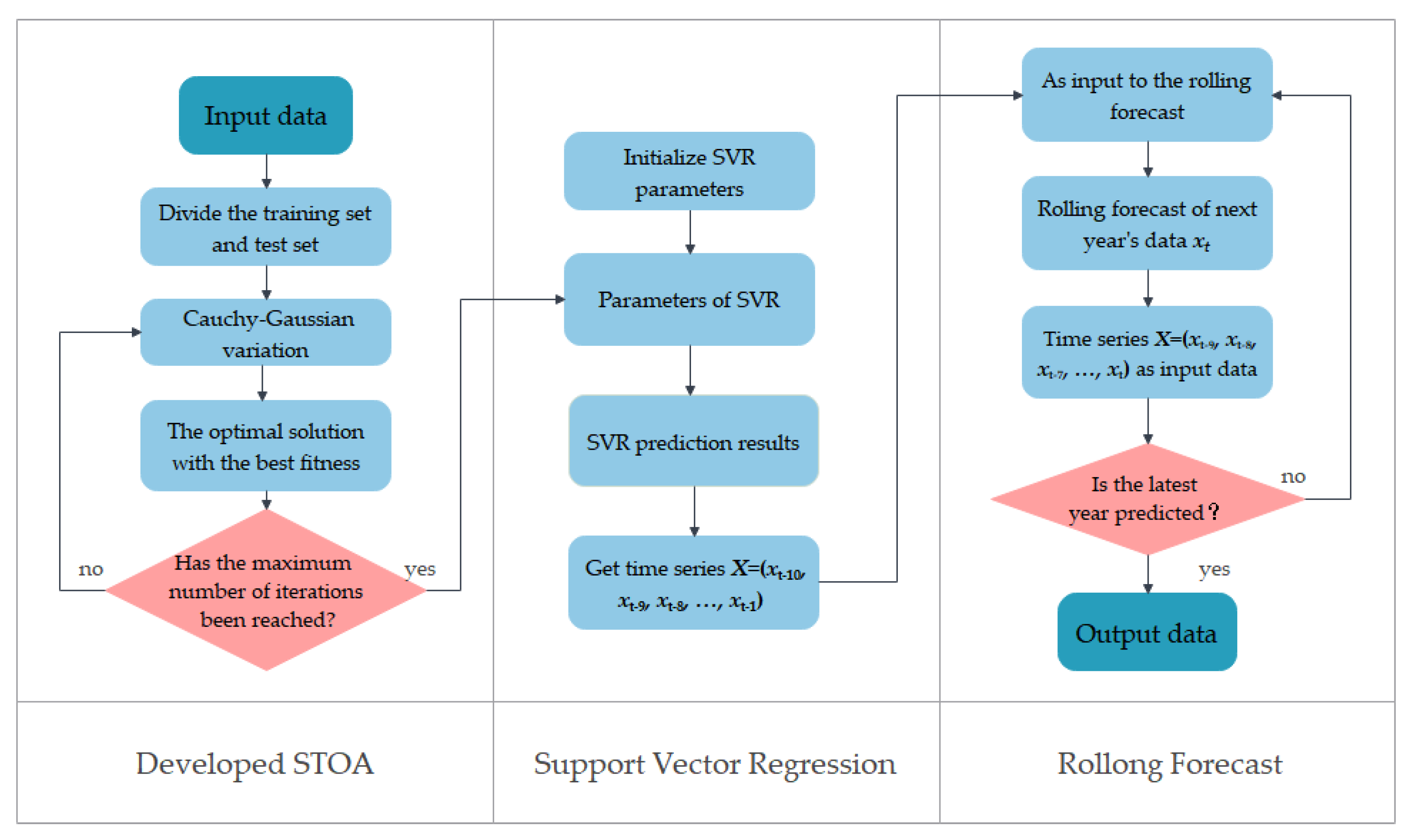
In this paper, an adaptive Gauss–Cauchy mutation operator is introduced to effectively increase the population diversity and search space and to improve the STOA, which is prone to local optimum problems. The key parameters of the SVR model are optimized by using the improved sooty tern algorithm so that the SVR model can mine the linear and nonlinear information in the data well. Through the optimized SVR rolling prediction model, the final temperature prediction results are obtained. The principle of an adaptive STOA-SVR rolling combination prediction model proposed in this study is shown in Figure 3.
As shown in Figure 3, the method used in this paper can be divided into three steps: Firstly, to avoid the possibility of the sooty tern algorithm stalling after finding the local optimal solution, the Gauss–Cauchy mutation operator is introduced on the basis of the traditional sooty tern algorithm. After each iteration, the improved sooty tern algorithm perturbs the current optimal individual position to obtain a new position. This perturbation strategy expands the search space and improves the global search capability of the algorithm. Secondly, it is found that the predictive performance of the SVR model is closely related to the choice of its super-parameters. Therefore, the improved STOA algorithm is introduced into the SVR model, and the optimized STOA algorithm is used to calculate the optimal parameters according to the training set data. Then, the optimal parameters obtained by the sooty tern algorithm are applied to the SVR model. According to the real-time updating and self-adjusting characteristics of rolling prediction, it is integrated into the SVM prediction model. Finally, an adaptive and optimized STOA-SVR rolling temperature prediction model is established based on the SVM, STOA and rolling prediction, and the global average temperature for the next 20 years is predicted.

4.1. SVR with Fusion Rolling Prediction

By using appropriate kernel function parameters, SVR can capture linear and non-linear relationships well in time series data and dig out historical laws of data, which has a very good effect on temperature prediction. By integrating rolling prediction into the SVR prediction model and using its real-time updating and self-adjusting principle, the prediction accuracy can be greatly improved.

4.1.1. Introduction of the SVR

In this paper, the main objective is to use the historical temperature data for fitting, find a function to fit the relationship between time and temperature series and expect to obtain a result with minimum fitting error so that this function can be used to predict the future temperature. This can be achieved by the SVM model [37], which mainly maps the input to a high-dimensional feature space by nonlinear mapping (kernel function) and then constructs the optimal classification hyperplane in this space. Therefore, it can provide the fitting equation with very high accuracy without worrying about local optimization and multicollinearity problems. For the existing global mean temperature data sample D, the expression of the optimization problem corresponding to SVR is as follows:
min w , b , ξ i , ξ ^ i 1 2 w 2 + C i = 1 m ( ξ i + ξ ^ i )
s . t . f ( x i ) y i ε + ξ i ,   0 ξ i ( i = 1 , 2 , , m ) y i f ( x i ) ε + ξ ^ i ,   0 ξ ^ i ( i = 1 , 2 , , m )  
where w is a weight vector that determines the direction of the hyperplane; C is a penalty factor and a non-negative relaxation variable; ε is an insensitive loss function and represents the allowable error between the regression value and the true value.
The Lagrange function is then introduced, the appropriate kernel function is determined according to the Karush–Kuhn–Tucker (KKT) condition and a series of transformations of the equation are performed to obtain the SVR regression function:
f ( x ) = i = 1 n ( α i α i ) K ( x i , x ) + b
where αi and  α i  are the Lagrange multipliers that satisfy the constraint conditions; K is the kernel function; b is the offset of the regression function.
The appropriate choice of penalty factor, insensitive loss function and kernel function is the key factor affecting the SVR function. The Gaussian radial basis kernel function (RBF) has the advantages of few parameters, low computational complexity and easy implementation, so in this study, the RBF function is selected as the kernel function of the SVR regression model to improve the prediction performance of global mean temperature. The expression of the RBF kernel function is:
K ( x i , x j ) = exp ( x i x j 2 / 2 δ )
where δ is the width parameter of the kernel function; xi is the input sample and xj is the center of the kernel function.

4.1.2. SVM Regression with Rolling Prediction

Traditional SVM prediction mainly uses static data sources in the data matrix for prediction analysis. Therefore, only the fixed temperature data from 1880 to 2022 is used for prediction, and the previously obtained prediction results cannot be incorporated into the updated data series. This may lead to an increase in the final error so that the accuracy of the long-term forecast results is seriously reduced.
Therefore, according to the real-time updating and self-adjusting application principle of rolling forecast, it is integrated into the SVM forecasting model, and the earliest data series is eliminated by using the updated data. By constantly updating the data formed at the next moment, a closed ring forecast structure is formed, and then a series of forecast data is obtained.
Finally, the temperature predicted by the model is compared with the actual temperature of the test set, and the error and goodness of fit are calculated to evaluate the accuracy of the model prediction. This process can effectively improve the prediction of the SVM. The specific steps are as follows:
Assuming that the rolling step size is N, the training set is divided into m sequences according to the rolling step size. The real data at the first N times of the i-th subsequence are known to be x1, x2, …, xN. The number of subsequences xN+1 at time N + 1 is predicted according to the data of the first N moments of the known subsequence. When time N + 1 is reached, the data of that time are added to the real data and the data farthest from the data point are removed. At this point, the time series is x2, x3, …, xN, xN+1. The time series at this point is then used to predict the output interval of the sub-series at time N + 2. The prediction is completed according to this rolling prediction mode. The input and output of the rolling prediction training set are shown in Equation (5).
X = x 1 x 2 x N x 2 x 3 x N + 1 x m x m + 1 x N + N 1 ,   Y = x N + 1 x N + 2 x N + m
where X is the training input sample and the training dimension is m × N; Y is the training output sample; the training dimension is m. The calculation of the training output sample is predicted by the SVM, and the prediction formula is as follows:
T x N + k = i = k N + k 1 ( α i α i ) K ( x i , x N + k ) + b
where  T x N + k  is the predicted mean temperature of year xN+k, and k is the k-th training output sample.

4.2. Improved STOA Optimization Algorithm

A large number of experimental experiences show that the main parameters affecting the SVR regression effect are the penalty factor C, the insensitive loss function ε and the width parameter δ of the kernel function.
The penalty factor C mainly determines the accuracy and degree of generalization of the model. If C is too large, the model will be very complicated and may cause overfitting problems; if C is too small, it is prone to underfitting problems. By controlling the size of the regression error, the insensitive loss function determines the number of support vectors that satisfy the condition. If ε is too large, the number of support vectors will be small, resulting in an overly simple model and a lack of learning accuracy. If ε is too small, the regression accuracy will be too high, but the model may be too complicated and the degree of generalization of the model will be reduced. The width parameter δ of the kernel function, which controls the radial range of the function, also has a great influence on the learning performance of SVR. Therefore, the selecting of a reasonable combination of parameters is a necessary condition for obtaining highly accurate regression results.
In this paper, the key parameters (C, δ, ε) of SVR were optimized using the sooty tern optimization algorithm (STOA), and a highly accurate SVR prediction model was established.

4.2.1. Traditional STOA Optimization Algorithm

STOA is a new optimization algorithm proposed by Himan and Kaaur [38] in 2019 for industrial engineering problems which is inspired by the foraging behavior of seabirds in nature. The sooty tern is an omnivorous bird that feeds on earthworms, insects, fish and other food. This algorithm has a strong global search capability and high precision. STOA is a population-based approach divided into a global search phase and a local search phase. The global search phase mainly consists of three parts: collision avoidance, convergence to the optimal solution and position update.
(1) For the collision avoidance, the following mathematical formula can be used:
B = γ × P ( k )
γ = α ( k × ( α M a x i t e r a t i o n ) )       k = 0 , 1 , 2 , , M a x i t e r a t i o n  
where B is the safe position to ensure no collision between black terns; P(k) is the current position of the black tern. γ is the collision avoidance factor; k is the number of iterations; α is set to 2.
(2) Convergence to the optimal solution can be expressed by Equation (9).
M = β × ( P b ( k ) P ( k ) ) β = 0.5 × r
where: M is the optimal position of the black tern colony; Pb(k) is the current optimal individual; β is a random regulator; r is a random number from [0, 1].
(3) The following formula can be used to update the position:
D = B + M
where D is determined according to the current position and optimal position of the sooty tern.
In the local exploration phase, the birds can use their wings to gain height and adjust their speed and angle of attack during migration. Their hovering behavior when attacking prey can be defined by the following mathematical model:
x = R × cos ( θ ) y = R × cos ( θ ) z = R × θ r = u × e k v
where R is the spiral radius; θ is the angle of attack; the range is [0, 2π]; u and v are spiral constants, set to 1. The formula for updating the position of the sooty tern can be expressed by Equation (12):
P ( k ) = ( D × ( x × y × z ) ) × P b ( k )

4.2.2. Improving the STOA Algorithm

In the late iteration period of the sooty tern optimization algorithm, the diversity of the sooty tern population weakens and individuals are easily accumulated during migration, so the probability of the algorithm falling into the local optimum solution is greatly increased. To prevent the algorithm from stagnating after finding the local optimum, some researchers introduced the Gaussian mutation strategy [39].
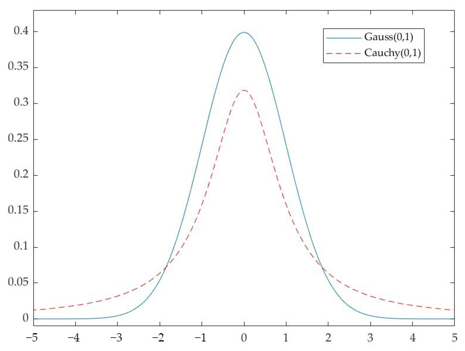
To solve the problem that the sooty tern optimization algorithm tends to fall into the local optimum solution in the late optimization period, an adaptive Gauss–Cauchy mutation operator is introduced in this paper. The main part of the Cauchy mutation operator is the Cauchy distribution. The Cauchy distribution is a special distribution in probability theory and mathematical statistics. It has no expectation and no mean, and its probability density function is large in the middle and small at both ends. The Cauchy distribution is particularly perturbed because of its unique structure of flat and long shapes at both ends. The probability density function of the standard Cauchy distribution is:
f ( x ) = 1 π ( x 2 + 1 )   x ( , + )
Figure 4 shows the probability density curve of the Cauchy and Gaussian distributions. The Cauchy distribution reaches its peak at the origin and extends smoothly from the peak to both ends. The peak value of the Gaussian distribution at zero is higher than that of the Cauchy distribution, and the speed of the Gaussian distribution extending to both ends is obviously faster than that of the Cauchy distribution, which will result in poor disturbance capability. Therefore, based on the Gaussian perturbation, the Cauchy variation is introduced into the sooty tern algorithm. After each iteration of the algorithm, the Cauchy variation is performed on the current optimal individual position to obtain a new position. If the new position after mutation is found to be better than the current individual position, the new position after mutation is selected to enter the next iteration. Such a perturbation strategy can effectively increase the diversity of the individual population, thereby expanding the search space and improving the global search capability of the algorithm. The optimal position is perturbed by Equation (14):
P ( k ) = P ( k ) × [ 1 + λ 1 C a u c h y ( 0 , 1 ) + λ 2 G a u s s ( 0 , 1 ) ] λ 1 = 1 t 2 / M a x i t e r a t i o n 2 λ 2 = t 2 / M a x i t e r a t i o n 2
where P(k)′ is the position after mutation in the t-th iteration; Cauchy(0,1) and Gauss(0,1) are random variables satisfying the Cauchy and Gaussian distributions, respectively. Maxiteration is the maximum number of iterations.
From the above equation, it can be analyzed that in the early iteration, the value of λ1 is large and Cauchy perturbation is mainly performed to allow STOA to search in a large area. At the later stage of the iteration, λ1 decreases while λ2 increases. At this point, the Gaussian perturbation plays a dominant role, which enhances the local search capability of the algorithm and significantly improves the convergence accuracy.

4.3. STOA-SVR Rolling Temperature Prediction Based on Adaptive Optimization

The time series in the global mean temperature problem studied in this paper obviously contains more than one data feature belonging to a complex nonlinear series. Using a single prediction model may not be able to describe each feature of the data well, resulting in some bias in the prediction result. The combination model can alleviate this problem to some extent. Since temperatures need to be predicted over several decades, using only data from the training set can lead to a serious loss of accuracy in the later stages of the prediction. Therefore, this paper advocates the method of rolling prediction, i.e., the temperature data of the first 10 years in the original data are used to predict the temperature value of the next year, which is then added to the original series as new data, and the data of the first year are deleted. By constantly updating the prediction, the data are formed at the next moment.
As mentioned above, the main parameters affecting the SVR regression effect are the penalty factor C, the insensitive loss function ε and the width parameter δ of the kernel function. Therefore, selecting an appropriate combination of parameters is a necessary condition for obtaining highly accurate regression results. In this paper, the key parameters (C, δ, ε) of SVR are optimized by the improved sooty tern algorithm, and a highly accurate SVR prediction model is established. Based on the above considerations, an STOA-SVR rolling temperature prediction model based on adaptive optimization is proposed in this paper:
T x N + k = i = k N + k 1 ( α i α i ) K ( x i , x N + k ) + b ( C , δ , ε ) = P ( k ) × [ 1 + λ 1 C a u c h y ( 0 , 1 ) + λ 2 G a u s s ( 0 , 1 ) ] P ( k ) = ( D × ( x × y × z ) ) × P b ( k ) K ( x i , x N + k ) = exp ( x i x N + k 2 / 2 δ )
where  T x N + k  is the predicted temperature in year xN+k, K is the Gaussian kernel function and δ is the optimal width parameter found after optimizing the STOA algorithm.

5. Results

Although SVR is a linear model, it can be extended to nonlinear cases by selecting appropriate kernel functions. This means that SVR is good at capturing both linear and nonlinear relationships in the data. Therefore, the research idea of this paper is to first use the improved STOA algorithm to optimize the parameters of the Gaussian kernel function of SVR, and then, based on the idea of rolling prediction, to use SVR to predict the trend of time series to obtain results.

5.1. SVR Parameter Solution Based on Enhanced STOA

Based on the above model, the STOA algorithm is used to solve for the optimal parameters of the SVR. The detailed procedure is shown in Algorithm 1:
Algorithm 1: SVR parameter solution based on improved STOA
Input: Data set D, population size N, maximum number of iterations Maxiterations, maximum Cmax and minimum Cmin of the penalty factor, maximum δmax and minimum δmin of the width parameter, and maximum εmax and minimum εmin of the insensitive loss function.
Output: The best parameter (C, δ, ε) best
1: procedure STOA
2: Initialize the parameters γ and β
3: Calculate the fitness of each search agent
4: (C, δ, ε) best the initial best search agent
5: Calculate adaptive weights λ1 and λ2
6: Update the positions by using Equation (14)
7: (C, δ, ε) best the best search agent after perturbation
8:   while (k < Maxiterations) do
9:       for each search agent do
10:       Update the positions of each agent by using Equation (12)
11:     end for
12:     Update the parameters γ and β
13:     Calculate the fitness value of each search agent
14:     Update (C, δ, ε) best if there is a better solution than previous optimal solution
15:     k ← k + 1
16:    end while
17: return (C, δ, ε) best
18: end procedure
In this paper, Python [40] was used to write the code of the STOA optimization algorithm, and the initial parameter was set as: population = 20; number of iterations = 200. The coefficient of the RBF kernel function of the SVR was assumed to be 10. Based on the adaptive STOA algorithm, when the optimal fitness value is 0.009279, the optimal parameter of SVR is: C = 101.2689; δ = 10−1.6491; ε = 5.5943.

5.2. Results of the SVR Rolling Forecast

To solve the problem of decreasing forecasting accuracy caused by long time series, the idea of rolling forecasting was adopted in this paper. The rolling step size was 10, which was used to predict the following year’s data with the data of the first 10 years and then solved again by Python. The prediction results based on the SVR model are shown in Figure 5.
It can be seen from Figure 5 that the model established in this paper is accurate in predicting the change trend of global mean temperature, and the predicted value has a high degree of agreement with the actual value, and the error of both is small, which indicates that the model established in this paper has a good prediction ability.

6. Discussion

To verify the accuracy and applicability of the STOA-SVR rolling prediction model for global mean temperature, several models were selected for comparative analysis of temperature prediction, and the prediction performance indices of each model were calculated. In addition, to verify the ability of the SVR model in this paper to capture the linear and nonlinear relationship in the data, the residual sequence obtained by the STOA-SVR model was considered to be modified by using the LSTM model to check whether the residual was sufficiently small.

6.1. Comparative Experimental Results and Error Analysis

In this study, the global mean temperature data set from 1880 to 2022 was used for analysis. The calculation results of the proposed method were compared with other traditional methods to verify the accuracy of the model.

6.1.1. Comparative Experimental Results

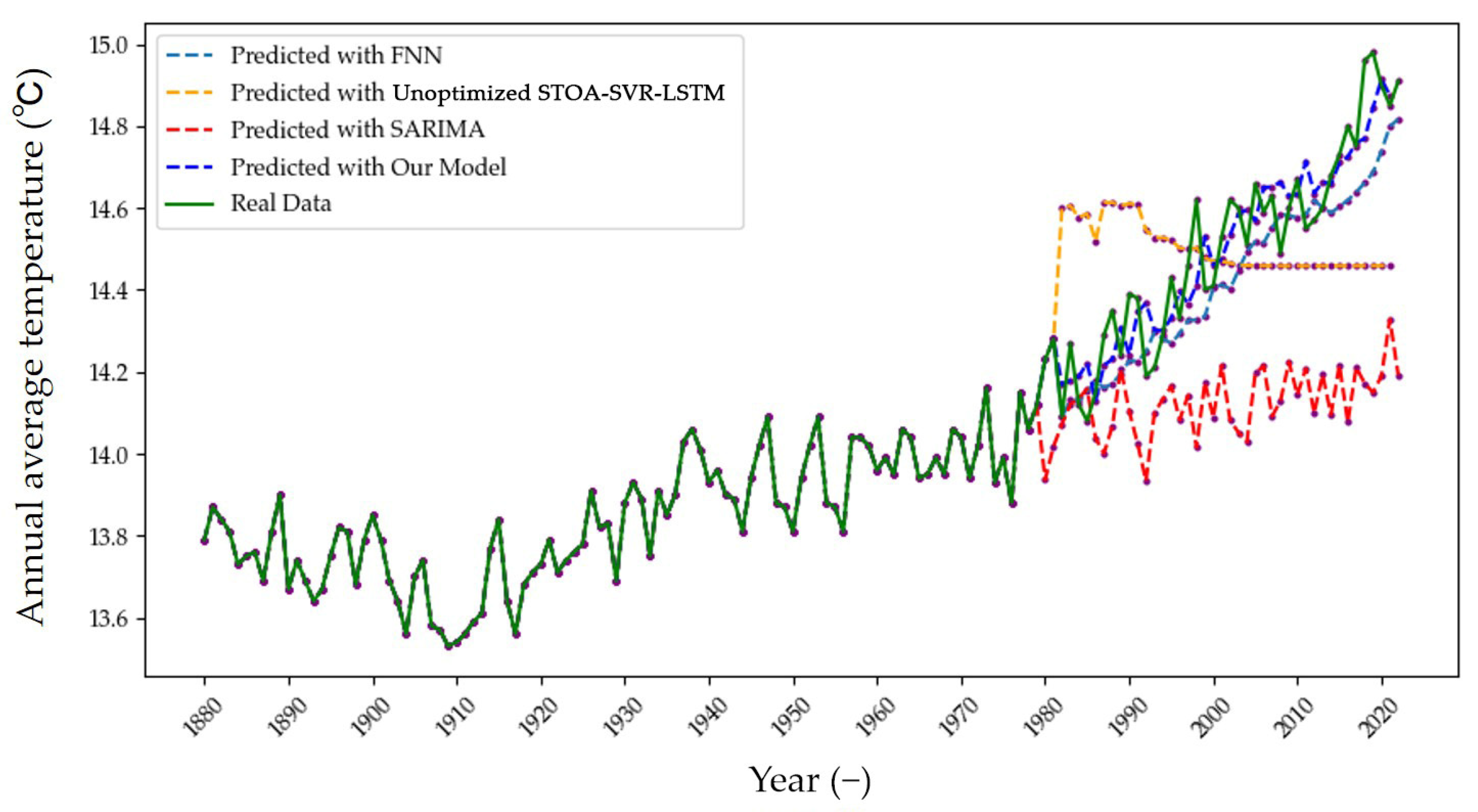
In order to verify the accuracy and effectiveness of the STOA-SVR model for temperature prediction, a single model SARIMA, a feedforward neural network FNN and a combined model SVR-LSTM under traditional STOA optimization were selected as comparative models in this study. The comparative prediction results of each model are shown in Figure 6.
The comparative experiments in this study were carried out under the Pytorch framework. In the SARIMA model, the parameters were (2, 1, 2) and the seasonal parameters were (1, 1, 1, 12). The number of iterations of the FNN is 100, the number of layers is three and the activation function is ReLU. In the unimproved STOA-SVR-LSTM model, the number of hidden layers of the LSTM is 2, the number of hidden layer neurons is 24 and the number of iterations is 200. Using the Adam optimizer, the penalty factor of the error term of the SVR model is 100.5, the coefficient of the kernel function is 100.5 and the degree of the polynomial kernel function is three by default.
As can be seen from Figure 6, compared with the single SARIMA, FNN and STOA- SVR-LSTM combined model, the STOA-SVR rolling temperature prediction model based on adaptive optimization proposed in this paper can better fit the data change trend of global mean temperature, and the prediction effect is better.

6.1.2. Error Analysis

To evaluate the temperature prediction performance of each model, three indices, root mean square error (RMSE), mean absolute error (MAE) and goodness of fit (R2), are selected as evaluation indices. The formulas are given in Equations (16)–(18):
R M S E = 1 N i = 1 N y i y ^ i 2
M A E = 1 N i = 1 N | y i y ^ i |
R 2 = 1 i = 1 n ( y i y ^ i ) 2 / i = 1 n ( y i y ¯ i ) 2
where yi and ŷi are the actual and predicted values of the global mean temperature in the test set, respectively; ȳi is the mean true temperature; N is the number of test samples.
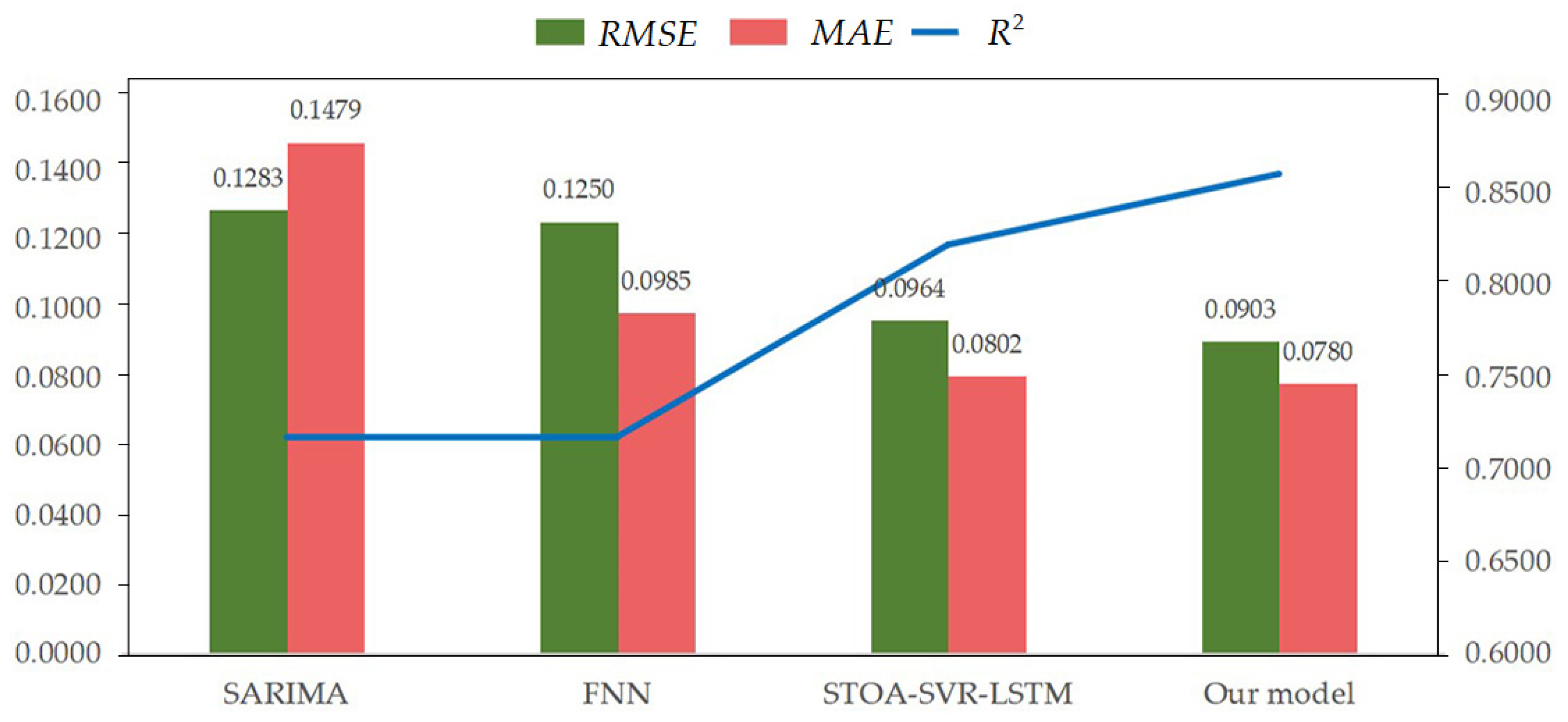
The prediction performance indicators of each model are shown in Table 2, and the difference comparison is shown in Figure 7.
As can be seen from Table 2 and Figure 7, the STOA-SVR-LSTM rolling prediction model proposed in this paper is the best model, followed by the unimproved combined prediction model, and the SARIMA model has the worst prediction performance. At the same time, the prediction results of both the SARIMA model and the FNN model are less accurate than the unimproved combined model, which also indicates that the combined model is better than the single model to some extent. Compared to these typical forecasting models, the accuracy of the improved model is significantly improved and the RMSE is reduced by 6.33–29.62%. The MAE is reduced by 2.74–47.27% and the R2 is increased by 4.67–19.94%. The comparison of the experimental results fully proves the correctness of the proposed model algorithm and its applicability to temperature prediction.

6.2. Prediction for the Next 20 Years

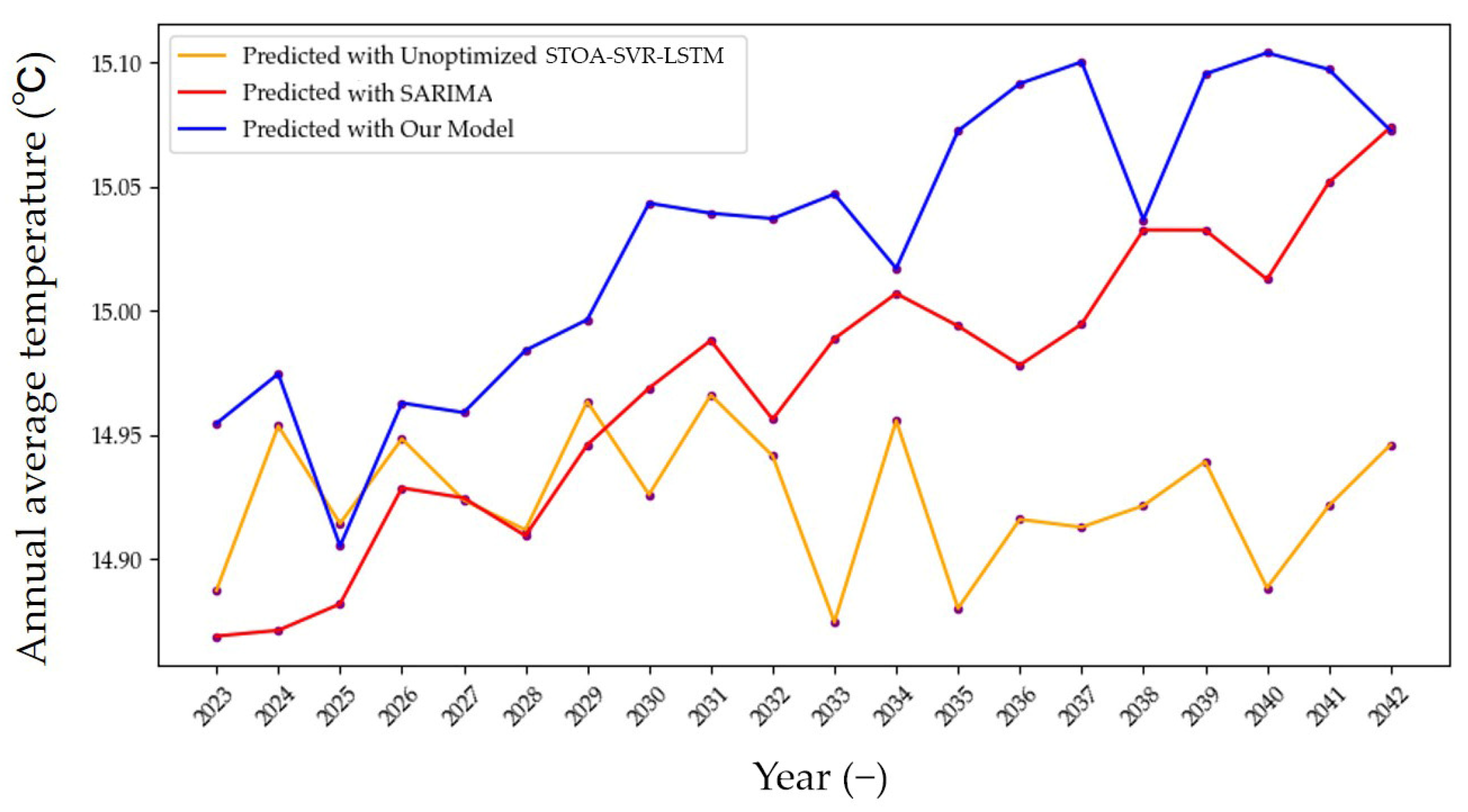
According to the above analysis results, it can be concluded that the model proposed in this paper has better temperature prediction ability. Therefore, this paper tries to apply it to predict the global annual mean temperature in the next 20 years to help people better understand the trend and possible impacts of future global climate change. In addition, the prediction of future temperature facilitates long-term planning and decision-making by governments and businesses to better cope with the challenges of climate change. The results predicted by the model are shown in Figure 8.
As can be seen in Figure 8, the global annual mean temperature for the next 20 years still shows an overall increasing trend, but the rate of increase is somewhat slower than that from 1880 to 2022, which may be due to the results of global policy adjustments such as “carbon peak and carbon neutrality” in recent years. In addition, the end of the projection has the characteristics of a “platforming” trend. Temperature stagnation has been a hot topic in the scientific community. Knight et al. [41] and Kerr et al. [42] conducted a comparative study of global temperature changes during 1998–2012 and the previous period based on global measured temperature data and reanalysis data, and they confirmed the existence of the phenomenon of climate warming stagnation. The Fifth Assessment Report of the IPCC [43] also clearly pointed out that the linear warming trend of global surface temperature during 1998–2012 has slowed down significantly compared with the previous 30–60 years, being about 1/3~1/2 of the warming rate during 1951–2012. According to the predicted results, this paper supports the view that the “warming hiatus” phenomenon is likely to occur in the next few decades and agrees that the possible causes are factors such as solar activity and volcanic eruption [44].
This paper predicts that the global annual mean temperature in the next 20 years will increase by 0.4976 °C compared to the global annual mean temperature in 1995–2014 (14.4930 °C), with an increase rate of 3.43%. IPCC AR6 [45] reports that the global annual mean temperature in the next 20 years will be 0.3–0.7 °C higher than that in 2001–2020 (14.6830 °C), and the calculated global mean temperature in 2021–2040 will be about 14.9374 °C, about 0.3 °C higher than that in 2001–2020. This is within the range of the report’s projections.

6.3. Modified Prediction Model Based on STOA-SVR-LSTM

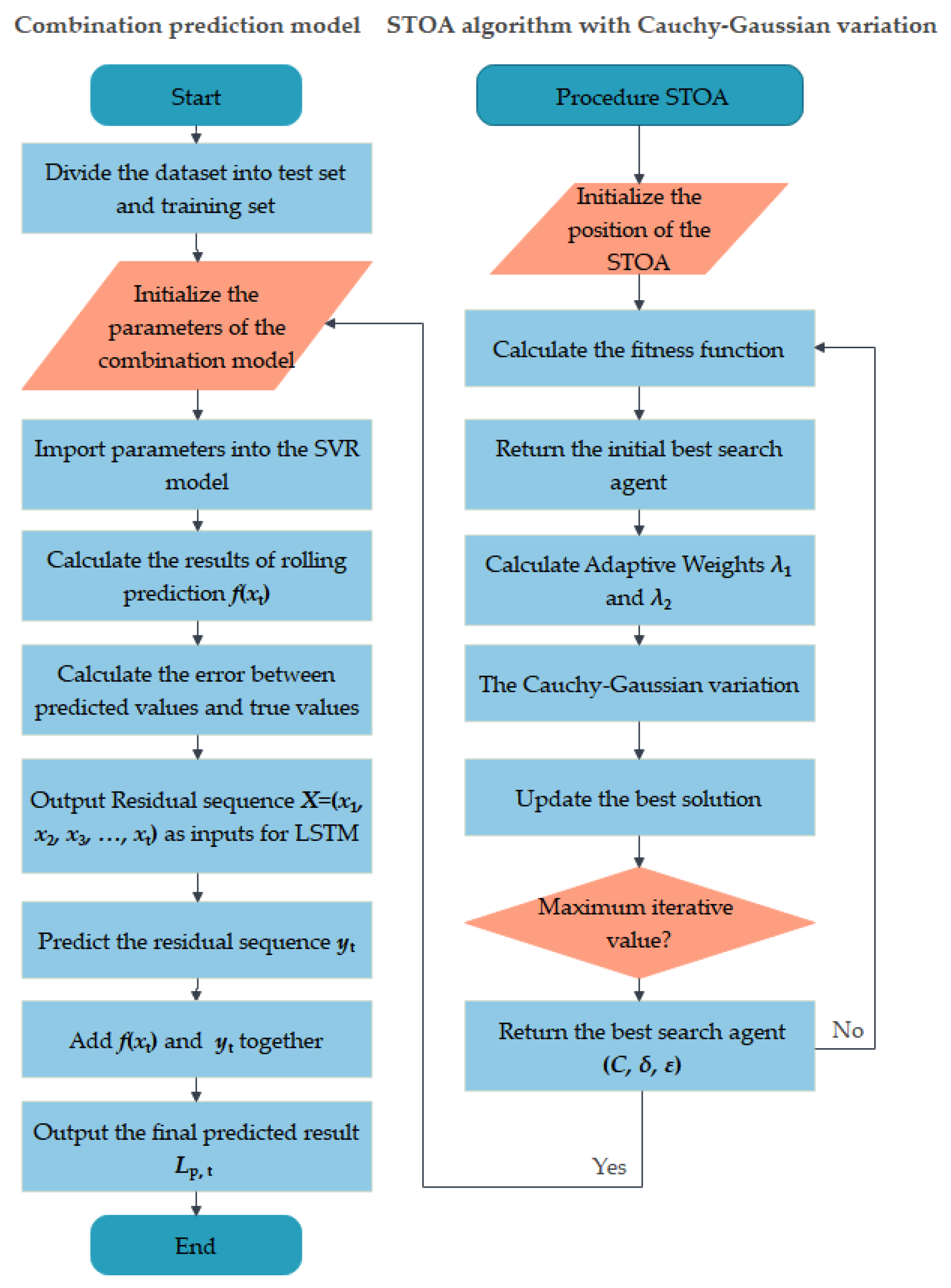
Although SVR is a linear model, after selecting the Gaussian kernel function and optimizing the parameters of the STOA algorithm, the model should be able to capture the linear and nonlinear relationship in the data well, and the influence of SVR residuals as nonlinear data on the prediction results should be very small. To verify this point, the LSTM model was used to modify the residual series obtained by the STOA-SVR model, and finally the two parts of the results were added in series to obtain the final temperature prediction results. This method fully accounts for the influence of the SVR prediction residual on the results. The algorithm flowchart of the model is shown in Figure 9.
Two hidden layers were set in the LSTM neural network, the number of hidden layer neurons was set to 24, Adam was used as the optimizer, the learning rate was set to 0.01 and MSE was used as the loss function. The residual sequence obtained from the STOA-SVR model was divided, with the first 70% as the training set and the last 30% as the best LSTM model to train the test machine. After many tests, the grid effect was best when the initial learning rate set in this paper was 0.01, the learning efficiency decreased after 100 trainings and the fading factor was 0.0106. The residual prediction result obtained by the LSTM neural network is shown in Figure 10.
It can be seen from Figure 10 that the predicted residual value has basically the same trend as the real value, and the predicted residual value is in the order of 10−4, which is very small. According to the calculation, the accuracy of the prediction results can only be improved by about 1% after the introduction of the LSTM model to correct the residual error, which has little impact on the final prediction results of temperature. From the above analysis, it can be concluded that after the parameter optimization of the STOA algorithm, the SVR model in this paper can capture the linear and nonlinear relationship in the data well and has a very good effect on temperature prediction.

7. Conclusions

In this study, we proposed an adaptive STOA-SVR rolling forecast combination model and trained the model using the global temperature data set from 1880 to 2022. The results were compared with other traditional methods, and temperature changes were predicted for the next 20 years. The main results are as follows:
(1)
A Cauchy–Gaussian variation was added to the sooty tern algorithm to ensure the diversity of the population and improve the ability of the algorithm to jump out of the local optimum. Then, the optimal parameters of the SVR model were obtained by using the improved STOA algorithm for rolling prediction to obtain the final prediction results.
(2)
Considering the influence of the SVR prediction residual on the results, the LSTM model was used to predict the residual sequence obtained by the STOA-SVR model, and the prediction accuracy was increased by about 1% by adding it to the prediction results obtained by the STOA-SVR model.
(3)
Three performance indices were used to evaluate the SARIMA, FNN, unimproved STOA-SVR-LSTM and improved STOA-SVR-LSTM models. The performance comparison of the prediction results shows that the STOA-SVR-LSTM rolling prediction model proposed in this paper can significantly improve the prediction accuracy.
(4)
The model predicts that the global mean temperature will increase by about 0.4976 °C in the next 20 years, with an increase rate of 3.43%.
Future work can be continuously improved with regard to the following aspects: First, the prediction model proposed in this paper has a good prediction effect on the global mean temperature data series, but the application of this model in different regions of the world needs further research; second, a variety of hybrid improvement strategies are explored to further improve the prediction accuracy; third, climate change not only causes the global annual mean temperature to continuously increase, but also increases the frequency of extreme weather events such as tornadoes and high temperatures. Since extreme weather is short-term weather, the time span of this study is one year, and the impact of extreme weather on global annual mean temperature change is not emphasized in this paper. Follow-up studies can comprehensively consider more extreme weather processes and try to dig deeper into the short-term temperature changes under different environments.

Author Contributions

Conceptualization, J.C.; methodology, J.C., S.S. and Y.D.; software, S.S. and Z.X.; validation, J.C., S.S. and Y.D.; formal analysis, J.C., S.S. and Y.D.; investigation, J.C., S.S., Y.D. and Z.X.; resources, J.C.; data curation, S.S. and Y.D.; writing—original draft preparation, J.C., S.S. and Y.D.; writing—review and editing, J.C., S.S., Y.D. and X.Q.; visualization, Y.D.; supervision, J.C.; project administration, J.C. and X.Q.; funding acquisition, J.C., S.S., Y.D., X.Q., S.S. and Y.D. contributed equally to this paper. All authors have read and agreed to the published version of the manuscript.

Funding

This research was funded by the Natural Science Foundation of Jiangsu Province (Grant Number: BK20190873), the Postgraduate Education Reform Project of Yangzhou University (Grant Number: JGLX2021_002), the Undergraduate Education Reform Project of Yangzhou University (Special Funding for Mathematical Contest in Modeling) (Grant Number: xkjs2022002) as well as the Lvyang Jinfeng Plan for Excellent Doctors of Yangzhou City.

Institutional Review Board Statement

Not applicable.

Informed Consent Statement

Not applicable.

Data Availability Statement

The data presented in this study are available upon request from the corresponding author.

Conflicts of Interest

The authors declare no conflict of interest.

References

  1. Purnadurga, G.; Lakshmi Kumar, T.V.; Koteswara Rao, K.; Rajasekhar, M.; Narayanan, M.S. Investigation of temperature changes over India in association with meteorological parameters in a warming climate. Int. J. Climatol. 2018, 38, 867–877. [Google Scholar] [CrossRef]
  2. Andronova, N.G.; Schlesinger, M.E. Causes of global temperature changes during the 19th and 20th centuries. Geophys. Res. Lett. 2000, 27, 2137–2140. [Google Scholar] [CrossRef]
  3. Li, M.; Liu, H.; Yu, S.; Wang, J.; Miao, Y.; Wang, C. Estimating the Decoupling between Net Carbon Emissions and Construction Land and Its Driving Factors: Evidence from Shandong Province, China. Int. J. Environ. Res. Public Health 2022, 19, 8910. [Google Scholar] [CrossRef]
  4. Kaminskiy, V.; Asanishvili, N.; Bulgakov, V.; Kaminska, V.; Dukulis, I.; Ivanovs, S. Impact of global and regional climate changes upon the crop yields. J. Ecol. Eng. 2023, 24, 71–77. [Google Scholar] [CrossRef]
  5. Miszuk, B.; Adynkiewicz-Piragas, M.; Kolanek, A.; Lejcuś, I.; Zdralewicz, I.; Strońska, M. Climate changes and their impact on selected sectors of the Polish-Saxon border region under RCP8. 5 scenario conditions. Meteorol. Z. 2022, 31, 53–68. [Google Scholar] [CrossRef]
  6. Harnack, R.; Harnack, J.; Lanzante, J.R. Seasonal temperature predictions using a jackknife approach with an intraseasonal variability index. Mon. Weather Rev. 1986, 114, 1950–1954. [Google Scholar] [CrossRef]
  7. Zhang, X.; Dang, Y.; Ding, S.; Wang, J. A novel discrete multivariable grey model with spatial proximity effects for economic output forecast. Appl. Math. Model. 2023, 115, 431–452. [Google Scholar] [CrossRef]
  8. Liang, L. A method of antarctic temperature forecasting based on time series model. In Proceedings of the 2017 5th International Conference on Frontiers of Manufacturing Science and Measuring Technology (FMSMT 2017), Taiyuan, China, 24–25 June 2017; pp. 1039–1043. [Google Scholar]
  9. Saha, A.; Singh, K.N.; Ray, M.; Rathod, S.; Dhyani, M. Fuzzy rule–based weighted space–time autoregressive moving average models for temperature forecasting. Theor. Appl. Climatol. 2022, 150, 1321–1335. [Google Scholar] [CrossRef]
  10. Möller, A.; Groß, J. Probabilistic temperature forecasting based on an ensemble autoregressive modification. Quart. J. R. Meteorol. Soc. 2016, 142, 1385–1394. [Google Scholar] [CrossRef] [Green Version]
  11. Shi, L.; Liang, N.; Xu, X.; Li, T.; Zhang, Z. SA-JSTN: Self-attention joint spatiotemporal network for temperature forecasting. IEEE J. Select. Top. Appl. Earth Observ. Remote Sens. 2021, 14, 9475–9485. [Google Scholar] [CrossRef]
  12. Kim, Y.; Mark Berliner, L. Bayesian state space models with time-varying parameters: Interannual temperature forecasting. Environmetrics 2012, 23, 466–481. [Google Scholar] [CrossRef]
  13. Fister, D.; Perez-Aracil, J.; Pelaez-Rodriguez, C.; Del Ser, J.; Salcedo-Sanz, S. Accurate long-term air temperature prediction with Machine Learning models and data reduction techniques. Appl. Soft Comput. 2023, 136, 110118. [Google Scholar] [CrossRef]
  14. Joshi, P.; Ganju, A. Maximum and minimum temperature prediction over western Himalaya using artificial neural network. Mausam 2012, 63, 283–290. [Google Scholar] [CrossRef]
  15. Wei, L.; Guan, L.; Qu, L. Prediction of Sea Surface Temperature in the South China Sea by Artificial Neural Networks. IEEE Geosci. Remote Sens. Lett. 2020, 17, 558–562. [Google Scholar] [CrossRef]
  16. Haq, M.A.; Ahmed, A.; Khan, I.; Gyani, J.; Mohamed, A.; Attia, E.A.; Mangan, P.; Pandi, D. Analysis of environmental factors using AI and ML methods. Sci. Rep. 2022, 12, 13267. [Google Scholar] [CrossRef] [PubMed]
  17. Alomar, M.K.; Khaleel, F.; Aljumaily, M.M.; Masood, A.; Razali, S.F.M.; AlSaadi, M.A.; Al-Ansari, N.; Hameed, M.M. Data-driven models for atmospheric air temperature forecasting at a continental climate region. PLoS ONE 2022, 17, e0277079. [Google Scholar] [CrossRef]
  18. Radhika, Y.; Shashi, M. Atmospheric temperature prediction using support vector machines. Int. J. Comput. Theory Eng. 2009, 1, 55. [Google Scholar] [CrossRef] [Green Version]
  19. Chen, Z.; Wang, Z.; Yang, Y.; Gao, J. ResGraphNet: GraphSAGE with embedded residual module for prediction of global monthly mean temperature. Artif. Intell. Geosci. 2022, 3, 148–156. [Google Scholar] [CrossRef]
  20. Aghelpour, P.; Mohammadi, B.; Biazar, S.M. Long-term monthly average temperature forecasting in some climate types of Iran, using the models SARIMA, SVR, and SVR-FA. Theor. Appl. Climatol. 2019, 138, 1471–1480. [Google Scholar] [CrossRef]
  21. Zhang, Z.; Dong, Y. Temperature forecasting via convolutional recurrent neural networks based on time-series data. Complexity 2020, 2020, 3536572. [Google Scholar] [CrossRef]
  22. Karevan, Z.; Suykens, J.A.K. Transductive LSTM for time-series prediction: An application to weather forecasting. Neural Netw. 2020, 125, 1–9. [Google Scholar] [CrossRef] [PubMed]
  23. Baareh, A.K.M. Temperature forecasting system using fuzzy mathematical model: Case study Mumbai City. Int. J. Appl. Evol. Comput. 2018, 9, 48–57. [Google Scholar] [CrossRef] [Green Version]
  24. Jin, Y.; Wang, R.; Zhuang, X.; Wang, K.; Wang, H.; Wang, C.; Wang, X. Prediction of COVID-19 data using an ARIMA-LSTM hybrid forecast model. Mathematics 2022, 10, 4001. [Google Scholar] [CrossRef]
  25. Su, S. Nonlinear ARIMA models with feedback SVR in financial market forecasting. J. Math. 2021, 2021, 1519019. [Google Scholar] [CrossRef]
  26. Guo, Y.; Tang, W.; Hou, G.; Pan, F.; Wang, Y.; Wang, W. Research on precipitation forecast based on LSTM–CP combined model. Sustainability 2021, 13, 11596. [Google Scholar] [CrossRef]
  27. Ji, R.; Shi, S.; Liu, Z.; Wu, Z. Decomposition-Based Multi-Step Forecasting Model for the Environmental Variables of Rabbit Houses. Animals 2023, 13, 546. [Google Scholar] [CrossRef]
  28. Roy, D.S. Forecasting the air temperature at a weather station using deep neural networks. Procedia Comput. Sci. 2020, 178, 38–46. [Google Scholar] [CrossRef]
  29. Xiao, C.; Chen, N.; Hu, C.; Wang, K.; Xu, Z.; Cai, Y.; Xu, L.; Chen, Z.; Gong, J. A spatiotemporal deep learning model for sea surface temperature field prediction using time-series satellite data. Environ. Modell. Softw. 2019, 120, 104502. [Google Scholar] [CrossRef]
  30. Yang, J.; Huo, J.; He, J.; Xiao, T.; Chen, D.; Li, Y. A DBULSTM-Adaboost Model for Sea Surface Temperature Prediction. PeerJ Comput. Sci. 2022, 8, e1095. [Google Scholar] [CrossRef]
  31. Nketiah, E.A.; Chenlong, L.; Yingchuan, J.; Aram, S.A. Recurrent neural network modeling of multivariate time series and its application in temperature forecasting. PLoS ONE 2023, 18, e0285713. [Google Scholar] [CrossRef]
  32. Tran, T.K.T.; Lee, T.; Shin, J.-Y.; Kim, J.-S.; Kamruzzaman, M. Deep learning-based maximum temperature forecasting assisted with meta-learning for hyperparameter optimization. Atmosphere 2020, 11, 487. [Google Scholar] [CrossRef]
  33. Tao, H.; Ewees, A.A.; Al-Sulttani, A.O.; Beyaztas, U.; Hameed, M.M.; Salih, S.Q.; Armanuos, A.M.; Al-Ansari, N.; Voyant, C.; Shahid, S. Global solar radiation prediction over North Dakota using air temperature: Development of novel hybrid intelligence model. Energy Rep. 2021, 7, 136–157. [Google Scholar] [CrossRef]
  34. Zhang, X.; Xiao, Y.; Zhu, G.; Shi, J. A coupled CEEMD-BiLSTM model for regional monthly temperature prediction. Environ. Monit. Assess. 2023, 195, 379. [Google Scholar] [CrossRef] [PubMed]
  35. Elshewey, A.M.; Shams, M.Y.; Elhady, A.M.; Shohieb, S.M.; Abdelhamid, A.A.; Ibrahim, A.; Tarek, Z. A Novel WD-SARIMAX model for temperature forecasting using daily delhi climate dataset. Sustainability 2022, 15, 757. [Google Scholar] [CrossRef]
  36. National Oceanic and Atmospheric Administration. Biden-Harris Administration Considers National Marine Sanctuary in Pennsylvania’s Lake Erie. Available online: https://www.noaa.gov/ (accessed on 21 April 2023).
  37. Üstün, B.; Melssen, W.J.; Buydens, L.M.C. Visualisation and interpretation of support vector regression models. Anal. Chim. Acta 2007, 595, 299–309. [Google Scholar] [CrossRef]
  38. Dhiman, G.; Kaur, A. STOA: A bio-inspired based optimization algorithm for industrial engineering problems. Eng. Appl. Artif. Intell. 2019, 82, 148–174. [Google Scholar] [CrossRef]
  39. Abdel-Basset, M.; Mohamed, R.; Mirjalili, S.; Chakrabortty, R.K.; Ryan, M.J. MOEO-EED: A multi-objective equilibrium optimizer with exploration–exploitation dominance strategy. Knowl.-Based Syst. 2021, 214, 106717. [Google Scholar] [CrossRef]
  40. Python Release 3.9.6. Available online: https://www.python.org/downloads/release/python-396/ (accessed on 20 May 2023).
  41. Knight, J.; Kennedy, J.J.; Folland, C.; Harris, G.; Jones, G.S.; Palmer, M.; Parker, D.; Scaife, A.; Stott, P. Do global temperature trends over the last decade falsify climate predictions. Bull. Am. Meteorol. Soc. 2009, 90, 22–23. [Google Scholar]
  42. Kerr, R.A. What happened to global warming? Scientists say just wait a bit. Science 2009, 326, 28–29. [Google Scholar] [CrossRef] [Green Version]
  43. IPCC. Climate Change 2013: The Physical Science Basis. Contribution to Working Group I to the Fifth Assessment Report of the Intergovernmental Panel on Climate Change; Cambridge University Press: Cambridge, UK; New York, NY, USA, 2013. [Google Scholar]
  44. Lean, J.L.; Rind, D.H. How will Earth’s surface temperature change in future decades? Geophys. Res. Lett. 2009, 36, L15708. [Google Scholar] [CrossRef] [Green Version]
  45. Zhou, T. New physical science behind climate change: What does IPCC AR6 tell us? Innovation 2021, 2, 100173. [Google Scholar] [CrossRef] [PubMed]
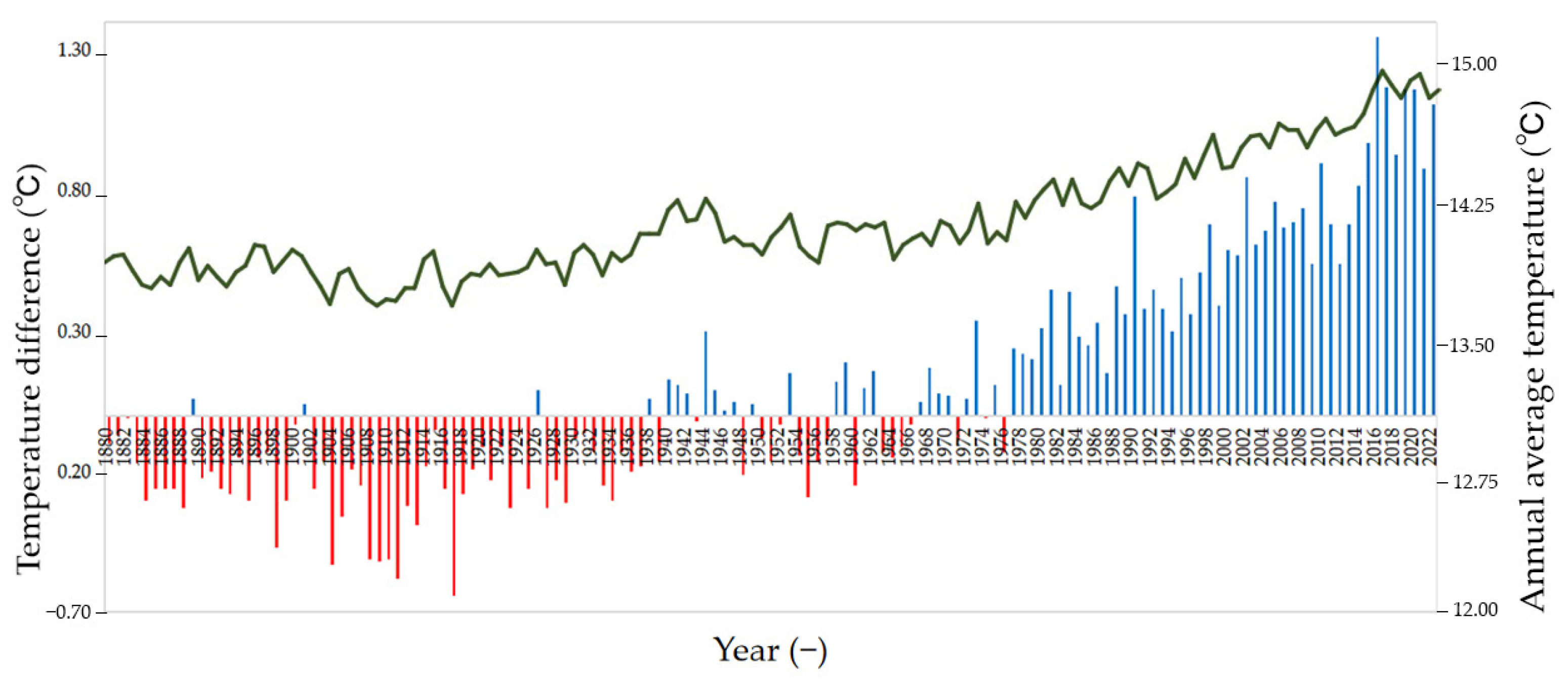
Figure 1. Differences and true values of global mean temperature from 1880 to 2022. The green line is the true global annual mean temperature, the red part of the cluster histogram indicates that the difference value is negative, blue is positive.
Sustainability 15 11068 g001
Figure 2. Series plot of the trend of temperature change, where (a) is the series plot of the long-term trend and (b) is the series plot of the seasonal trend.
Sustainability 15 11068 g002
Figure 3. Schematic diagram of the rolling combination prediction model.
Sustainability 15 11068 g003
Figure 4. Probability density function curves of the standard Cauchy and Gaussian distributions.
Sustainability 15 11068 g004
Figure 5. Prediction results of the SVR model. The points on the green line and the dashed red line represent the predicted and the real values.
Sustainability 15 11068 g005
Figure 6. Comparison of prediction results of different models. The points on the green line represent the real value. The points on the dashed sky blue, yellow, red and blue lines represent the predicted values with FNN, unoptimized STOA-SVR-LSTM, SARIMA and our model, respectively.
Sustainability 15 11068 g006
Figure 7. Comparison of prediction performance of different models.
Sustainability 15 11068 g007
Figure 8. Projected global mean temperature for the next 20 years. The points on the yellow, red and blue lines represent the predicted values with unoptimized STOA-SVR-LSTM, SARIMA and our model, respectively.
Sustainability 15 11068 g008
Figure 9. Flowchart of the STOA-SVR-LSTM algorithm.
Sustainability 15 11068 g009
Figure 10. LSTM residual prediction results. The points on the blue and green lines represent the predicted and real residuals.
Sustainability 15 11068 g010
Table 1. Comparison between the main methods used in the existing literature.
MethodsAdvantagesDisadvantages
Mathematical statistical-based forecasting methods① The main models include time series models, gray prediction, differential equation models, etc. These models can fully utilize data information, compute faster, require less data and can determine model parameters dynamically.
② Some models can show a significant relationship between dependent variables and independent variables and have good statistical properties.
① Over-reliance on existing data can lead to large errors in long-term forecasting and is only suitable for short-term forecasting.
② The model is relatively simple, the factors considered are insufficient and the forecasting results are one-sided.
③ Most mathematical statistical models are linear models that cannot capture non-linear segments of complex time series.
Machine learning-based methods① The main models include ANN, CNN, RNN, LSTM, GA models, etc. The computation is simple, with strong robustness, memory, and strong self-learning ability.
② Some machine learning, such as SVM, is easy to find the global optimal solution; suitable for small samples.
① Sensitive to the selection of some hyper-parameters, which requires tedious parameter adjustment.
② For some algorithms, such as neural network and GA, the learning process inside the model cannot be observed; the output results are difficult to predict.
③ Learning time is too long, may not achieve the purpose of learning.
Combination of different methods① Combined with the advantages of mathematical statistics and machine learning, it can capture the overall change rules of data sets with complex motion laws and reduce information loss.
② It has higher prediction accuracy and stability than a single prediction model.
It is necessary to select multi-dimensional and huge training data for model construction to improve the reliability of the model and greatly increase the computational complexity.
Table 2. Results of the prediction performance indicators for each model.
MethodsSARIMAFNNUnimproved STOA-SVR-LSTM ModelOur Model
RMSE0.12830.12500.09640.0903
MAE0.14790.09850.08020.0800
R20.71720.71750.82180.8722
Disclaimer/Publisher’s Note: The statements, opinions and data contained in all publications are solely those of the individual author(s) and contributor(s) and not of MDPI and/or the editor(s). MDPI and/or the editor(s) disclaim responsibility for any injury to people or property resulting from any ideas, methods, instructions or products referred to in the content.