Article

A Robust Stochastic Programming Model for the Well Location Problem: The Case of The Brazilian Northeast Region

by
Dayanna Rodrigues da Cunha Nunes
*,
Orivalde Soares da Silva Júnior
,
Renata Albergaria de Mello Bandeira
and
Yesus Emmanuel Medeiros Vieira
Postgraduate Program in Transport Engineering, Military Institute of Engineering, Rio de Janeiro 22290-270, Brazil
*
Author to whom correspondence should be addressed.
Sustainability 2023, 15(14), 10916; https://doi.org/10.3390/su151410916
Submission received: 16 May 2023 / Revised: 5 July 2023 / Accepted: 6 July 2023 / Published: 12 July 2023

Abstract

:
Slow-onset disasters, such as drought, are usually more destructive in the long term since they affect the productive capacity of a community, thereby preventing it from recovering using its resources. This requires the leaders and planners of drought areas to establish the best strategies for effective drought management. In this direction, the present work develops a robust stochastic programming approach for the problem of locating artesian wells for the relief of drought-affected populations under uncertainty. Our model considers different demand scenarios and proposes a novel perspective which considers both social and hydrogeological aspects for the location choice, aiming to maximize the affected area’s satisfaction through its prioritization using a composite drought risk index as well as to maximize the probability of success in water prospecting. We present a case study of our robust stochastic optimization approach for the Brazilian Semiarid Region using demand points from the database of Operação Carro-Pipa. Our findings show that a robust solution has a better expected value for the objective function considering all scenarios, so it can help decision makers to plan facility location and demand allocation under demand uncertainty, pointing out the best solution according to their degree of risk aversion.

1. Introduction

Drought is a recurrent natural phenomenon characterized by a rainfall reduction in comparison to regular pluviometric levels for a specific area, making the available water insufficient to meet human and environmental needs [1]. It is considered a hazard when it occurs intensively and extensively in densely populated areas. Moreover, when it exceeds the community’s capacity to respond to the hazard, it can result in a disaster, leading to economic, human, and environmental impacts which undermine human physical, mental, and social well-being [2].
A disaster can be understood as a disruption that affects a community as a whole. It can be natural or man-made. It can be slow onset, such as famine and drought, or sudden onset, such as tsunamis and earthquakes [3]. Slow-onset disasters usually have a more extensive impact and can be more destructive in the long term as they diminish the rates of savings, investment, demand, and productive capacity of the affected community [4].
Drought is among the disasters that have major impacts on society and ecosystems. For instance, the 2012 US drought and the 2010–2011 East Africa drought caused huge economic losses and famine around the world [5]. According to the Brazilian Atlas of Natural Disasters [6], drought is the disaster that most affects the Brazilian population due to its recurrence and intensity. From 1991 to 2010, there were close to 17,000 drought events recorded in 2944 municipalities, representing more than 50% of all disasters registered in the country for that period [7]. In Semiarid Northeast Brazil, the drought that occurred between 2012 and 2017, considered the most severe of the last 30 years, has affected about 1100 municipalities (about 20 million people per year) of the region. This prolonged drought caused economic losses of USD 6 billion due to its impacts on the agricultural sector [8,9,10].
Moreover, due to climate change, drought is expected to become more recurrent and severe in the context of climate change, with higher temperatures, more extreme precipitation regimes, and limited and uncertain water sources. On the other hand, water demand is expected to increase due to population growth. Therefore, leaders and planners in drought-prone regions must establish appropriate and innovative strategies for drought mitigation and preparedness [11].
Disaster Management (DM) activities are generally grouped into four phases: mitigation, preparedness, response, and recovery [12]. The author of [13] defines these phases as follows: mitigation aims at the reduction of the probability of disaster occurrence or the degree of its impacts, or both; preparedness consists of planning activities to be conducted after a disaster in order to increase the chances of survival and minimize financial and human losses; response considers action to reduce or eliminate the impact of disasters during their aftermath to prevent further suffering, financial loss, or other losses; and recovery regards recovering the area affected by a disaster. Humanitarian logistics is involved in three stages of DM, which are preparedness, response, and recovery [14].
Due to the increasing number and severity of recent disasters, researchers have given more attention to DM focused on humanitarian logistics. The surveys in this field have tended to employ modeling and optimization to solve such problems. In this regard, facility location models that involve locating distribution centers, warehouses, and other facilities are important for effective and efficient DM [14] since decisions involving the location of facilities are costly and long lasting, with impacts on numerous operational and logistical decisions [15].
Well drilling has been adopted as a measure to cope with drought in the Brazilian Semiarid Region since the 19th century [16]. However, a recurring challenge in the drilling of artesian wells in arid regions concerns their location; in other words, the choice of the most likely points to obtain productive wells. In hard rock terrains, groundwater occurs essentially confined to fractured and weathered horizons [17]. Fractured hard rock aquifers are non-extensive, irregular, anisotropic, and inhomogeneous, which may yield a relatively small amount of water [18]. They often present limited flow rates as well as high ionic concentrations (brackish water) and, thus, are not recommended for human consumption [16]). As a result, groundwater exploration without a previous hydrogeological survey often leads to failure due to the complex nature of groundwater occurrence in hard rock terrains [19].
In addition to the hydrogeological challenge, financial difficulty also exists since drought risk mitigation measures usually have a budget constraint. Hence, drought risk assessment can play an important part in drought management concerning prioritizing the most affected people in the choice of points for locating water wells. Drought indices are the most commonly used tools for drought evaluation [20]. Knowing that risk is a combination of both the region’s exposure to the natural event (hazard) and society’s vulnerability to the event [21], composite indices are the most recommended since they combine indicators that help to identify evidence of drought with those concerning local community vulnerabilities [22,23].
Finally, humanitarian logistics deals with a high level of uncertainty, mainly regarding demand, supply, and costs [24]. Therefore, when it comes to modeling and optimization applied to humanitarian operations planning, data uncertainty has a strong influence on the performance of these models and not considering it can lead to poor solutions [25]. In such cases, a mathematical approach that produces solutions less sensitive to the uncertainty data is preferred [26].
In this context, we propose two models, a deterministic one and a robust one, which deal with demand uncertainty, to address the location problem of artesian wells. The aim is to address both objectives of increasing the success rates in obtaining productive wells in hard rock terrains and prioritizing the communities most affected by drought. For the first objective, we use the model developed by [27], based on logistic regression, to consider the probability of occurrence of groundwater at the candidate points for locating a well. For community prioritization, we adopt the drought composite index (DCI) proposed by [23], a combination of both hazard and vulnerability. The proposed model was applied to a case study involving 739 points in the Brazilian Semiarid Region.
After this introduction, the remainder of the paper is organized as follows. Section 2 presents a literature review concerning the facility location problem and robust optimization. In Section 3, the proposed model for artesian wells’ location is described. Section 4 presents an application of the proposed model in a case study regarding the water distribution for beneficiaries in the Brazilian Semiarid Region, as well as the results and their analysis. Finally, the concluding remarks and possibilities of future research on the topic are presented in Section 5.

2. Literature Review

2.1. Facility Location Problem

Facility Location Problems (FLPs) lie in finding the best location for a set of facilities to serve a set of demand points. The best location is determined according to the constraints and the objective function of the problem [28].
Researchers [29,30] introduced the problems of p-center and p-median, both of which aim to find the optimal location of p facilities on a network considering some objective function. The former aims to minimize the maximum distance between any demand point and the closest facility to it while the latter minimizes the sum of the distances from each demand point to the closest facility. The authors of [31] modeled the location of emergency facilities as a Set Covering Problem (SCP) in which the sets comprise the potential facility points within a specified distance of each demand point. To ensure that, a coverage constraint is written for each demand point. The objective is to find the minimal number of facilities, which ensures that all demand points are covered and that the maximal service distance is respected.
Researchers [32] studied a particular case in which facilities are insufficient to achieve total coverage within some distance goal. The authors designated that problem as the Maximal Covering Location Problem (MCLP) which aims to maximize coverage within the desired service distance by locating a fixed number of facilities. Moreover, [33] presented the Uncapacitated Facility Location Problem (UFLP) applied to the problem of optimally locating bank accounts to maximize clearing times. The problem involves minimizing the sum of the fixed cost of maintaining an account in some cities and the cost of paying clients in some cities from an account in another city. In its formulation, there is no limitation for the capacity of a located facility. However, in most real-world problems, considering capacitated facilities is more realistic.
In the same way that simple formulation changes can easily extend basic models to account for setup and/or service costs they can also incorporate facility capacities. In such models, known as the Capacitated Facility Location Problem (CFLP), a set of constraints is added to the problem formulation so that the sum of the demands assigned to each facility does not exceed its capacity. For instance, that exact procedure was carried out by [34] to present capacitated versions of SCP and MCLP. Later on, [35] extended the classical CFLP to include facility sizes.
When it comes to solution methods, many realistic problems are not “integer-friendly” and so require the use of heuristics and metaheuristics. Among them are Genetic Algorithms (GA) and Tabu Search (TS). For example, [36] proposed a genetic algorithm for the p-median problem and [37] presented a Variable Neighborhood Search and two Tabu Search heuristics for the p-center problem. There are also a few Decision Support Systems (DSS) to solve general FLPs. SITATION is a solver provided by [38] which can solve p-center, p-median, SCP, MCLP, and UFLP to a maximum of 150 locations. Orloca (Operations Research LOCational Analysis Models) applies algorithms to solve the Fermat–Weber minisum location problem [39]. The Library of Location Algorithms (LoLA) can solve a larger set of problem types [40]. In that direction, [41] developed an open-source spreadsheet-based Decision Support System for facility problems, called the FLP Spreadsheet Solver, which can solve all the basic location problems mentioned above. It uses a Tabu Search algorithm and can find near-optimal solutions for problems with up to 200 locations.
Facility location problems can be studied using different approaches, considering uncertainties or not, involving one or more objectives, and their applications cover a wide variety of fields. The authors of [42] addressed them in vehicle reverse logistics; [43] in the food sector; [44,45,46,47] in the closed-loop supply chain; [48,49] in an RFID-based meat supply chain; [50] in the location and allocation of grain silos; [41,51,52] in the location of healthcare facilities; and [53,54,55,56,57] in humanitarian logistics.

2.2. Robust Optimization

As mentioned above, facility location decisions are characterized by the high costs associated with property acquisition and construction, making them long-term investments. To assure profitability, facilities need to be designed to remain in operation for an extended period. Thus, decision makers must choose locations to perform well according to the current state and that continue to be profitable as environmental factors change, populations shift, and market trends evolve. Finding robust facility locations is, then, a difficult task, demanding decision makers to account for uncertain future events [15].
For optimization under uncertainty, there are two approaches. The first one is stochastic optimization in which the uncertain parameters are associated with a probability distribution. The second one is robust optimization which presumes that the probability distribution function is unknown and then the uncertain parameters are identified using discrete scenarios or continuous ranges [14]. The latter considers the risk aversion of the decision maker to find solutions that are less affected by scenario changes [58]. Next, we present some papers that address robust optimization.
The authors of [59] defined two types of robustness for a solution to an optimization problem, which are solution robustness and model robustness. The former refers to the optimality of the solution—in other words, if it remains close to optimal for all scenarios; and the latter is related to feasibility—namely, if it remains almost feasible for all scenarios. They then introduced a general model formulation, called robust optimization (RO), that includes these two conflicting objectives, weighted by a parameter intended to capture the modeler’s preference between the two. Considering the complexity of the nonlinear model proposed by [59], [26] presented a more computationally efficient RO model, transformed into a linear program by the addition of n + m deviation variables (where n and m are the numbers of scenarios and total control constraints, respectively) instead of the 2n + 2m variables required by the approach of [59].
In the field of humanitarian logistics, [60] developed a multi-objective robust stochastic programming approach for disaster relief logistics based on Mulvey’s model and, to cope with the computational complexity due to its nonlinearity, they adopted Yu and Li’s formulation. The authors considered not only demands but also supplies and the cost of procurement and transportation as uncertain parameters. Their model attempts to minimize the total cost of the relief chain while maximizing the affected areas’ satisfaction. Other authors have also used a robust approach applied to humanitarian logistics, such as [54,55,61].

2.3. Research Gaps and Innovations

As mentioned above, the facility location problem has a wide area of application. However, when it comes to well location for groundwater exploitation, there is still limited research. We now present the most related works found in the literature.
The authors of [62] presented a multi-objective mixed integer linear programming model to determine the location and size of pumping facilities, considering their area of influence, to supply a set of demand points with water from an aquifer. The model considers the effect of groundwater extraction on the piezometric surface to avoid overexploitation of aquifers. Later, [63] applied the same model to a case study concerning the Querença-Silves aquifer in Portugal. The problem involved 10 demand points and 100 potential locations for the wells. The model was tested for different values for the maximum number of wells (5, 15, and 25) and Pareto optimal solutions were obtained using the ε-constraint method. The study showed that the model provides results consistent with the proposed objectives.
Meanwhile, [64] proposed an improved Tabu Search (TS) algorithm for solving facility location problems involving water infrastructure planning. The algorithm incorporates elements of a Variable Neighbourhood Search (VNS) metaheuristic, which makes the neighborhood expansion according to a ranking of potential locations.
Furthermore, [65] addressed the issue of water security in a coastal area subject to high groundwater salinity and large social inequalities. For this purpose, they developed a multi-objective optimization model to analyze the trade-offs between two objectives: maximizing overall access and maximizing low-income population access to an improved water supply. The optimization model considers groundwater salinity measurements, an extensive household survey, an audit of drinking water infrastructure, and the costs of a variety of supply options such as deep tube wells, desalination plants, and piped systems.
Even though the study of [65] considered low-income population access to water, which is one aspect that our work takes into consideration, none of the studies developed a model that could assist in the selection of the most susceptible points for productive wells and, at the same time, prioritize the communities most affected by water scarcity, as we propose in this paper. In addition, our work fills a research gap in this area by adopting a stochastic approach by considering the demand uncertainty, which is a common concern in such humanitarian efforts.

3. Model Formulation

This section describes the proposed models to solution the problem concerning the location of artesian wells. The problem is modeled as a mixed-integer programming (MIP) and concerns the choice of the location and the number of wells to be drilled in order to meet the water demand of the drought-affected population. Both models aim to maximize the water demand covered, increasing the success rates in obtaining productive wells, by considering hydrogeological parameters as well as prioritizing communities in locations with higher risk of drought. Section 3.2 presents a deterministic model that is then improved to a robust model, considering the uncertainty of demand, in Section 3.3. Finally, Section 3.4 presents the solution approach used to solve the problem. First, though, an explanation of the problem is provided in Section 3.1.

3.1. Problem Statement

The problem lies in locating several artesian wells to supply a certain set of demand points (cisterns) with water. The vertices considered for locating wells are distributed in three sets: vertices that already are wells ( V 1 ); vertices that are potential locations to wells ( V 2 ); and vertices that cannot be wells ( V 3 ). Figure 1 illustrates the well–cistern allocation and the chosen locations for the wells, represented by arrows, for an example involving 100 cisterns and 30 artesian wells. Note that the vertices that cannot be wells are not allocated to any cistern, not being chosen to locate a well.

3.2. Deterministic Model

This section presents a deterministic model to better understand the problem. Its formulation is based on the integer programming formulation of the underlying facility location problem proposed by [41]. Some modifications were made to adapt it to the problem at hand. First, in order to work with a single objective function, we considered the setup and transport costs as constraints of our model and the maximum distance was removed from the objectives because, to some extent, it is already contemplated by the transport cost. Another modification concerns the objective function of maximum demand coverage. While [41] considered the probability of a facility covering the demand in a certain location, we instead consider the probability of occurrence of groundwater. Furthermore, we have introduced a parameter related to the composite drought risk index, seeking a way to prioritize the locations most affected by the drought.
Consider a directed graph G = V , A , where the vertex set V, indexed by i and j, is the union of three disjoint subsets V 1 , V 2 , and V 3 . The first subset V 1 consists of vertices that already are wells. The second subset V 2 is composed of vertices that may be wells; in other words, vertices whose probability of occurrence of groundwater is greater than or equal to 50%. The third subset V 3 contains the vertices that cannot be wells; in other words, vertices whose probability of occurrence of groundwater is less than 50%. The probability of occurrence of groundwater p j was estimated using Equation (1) from the prospective model developed by [27] using the same study area considered in this paper. The model proposed by [27] is based on logistic regression and considers the following independent variables: the lithotype ( l i t j ); the lineament density ( l i n j ); the surface drainage ( d r e n j ); and the distance from the closest structural lineament ( d i s t j ). The independent variables chosen to compose this equation are the result of a vast literature review and statistical analysis carried out by [27]. Moreover, regarding the choice of the cut-off value of 50% for the composition of the subsets V 2 and V 3 , it was based on the definition proposed by [27] for the dependent variable of their prospective model in order to characterize it as a dichotomic variable. The arc set A contains all arcs connecting the vertices in V, including self-arcs i , i   i V .
p j = e 5.943   +   0.853   ×   l i t j   +   0.537   ×   l i n j   +   0.101   ×   d r e n j   +   2.739   ×   d i s t j 1   +   e 5.943   +   0.853   ×   l i t j   +   0.537   ×   l i n j   +   0.101   ×   d r e n j   +   2.739   ×   d i s t j
Each vertex i V has a demand q i and a drought composite index I R i , related to the municipality to which it belongs. The composite index that was considered in this paper is the one proposed by [23], which is the product of the region’s exposure (hazard) and the society’s vulnerability to drought. The hazard index takes into account the precipitation, evapotranspiration, temperature (average, maximum, and minimum), relative humidity, total insolation, and wind speed [66]. The vulnerability index considers exposure, sensitivity, and adaptive capacity. Both indices are composed of multiple indicators, selected based on a literature review, and weighted through the AHP (Analytic Hierarchy Process) method.
Moreover, each vertex j V has a probability of occurrence of groundwater p j , estimated by Equation (1), a setup cost s j , that is incurred if j is selected to host a well, and a capacity Q j . We denote the maximum service distance as δ. Associated with every arc i , j A , there is a distance d i j and the average cost of transport is denoted by c. We also add a budget limit to setup costs and transportation costs, referred to as S c and T c , respectively.
Let us define x i j to be equal to 1 if vertex i is served by a facility in j, and 0 otherwise. In addition, let us define y j to be equal to 1 if vertex j is going to locate a well, and 0 otherwise. Table 1 summarizes the notations used in the development of the deterministic model. The model is then defined by the expressions 2 to 12.
M a x i m i z e   z = i V j V q i × p j × I R i × x i j
s.t:
j V x i j 1     i V
x i j y j     i ,   j V
i ϵ V q i × x i j Q j × y j     j V 1 V 2
j V y j × s j B p
i V j V q i × d i j × c × x i j B d
x i j = 0     i , j V   |   d i j > δ
x i j 0,1     i , j V   |   d i j δ
y j = 1     j V 1
y j 0,1     j V 2
y j = 0     j V 3
The objective function (Equation (2)) aims to maximize the water demand ( q i ) covered while prioritizing demand points in locations with higher risk of drought ( I R i ) and drilling candidate points more likely to obtain a productive well ( p j ). Constraint 3 establishes that a cistern cannot be assigned to more than one well. Constraint 4 requires a well to be located at vertex j for any cistern i to receive service from it. The demand assigned to each well is required to be less than or equal to its capacity by constraint 5. Constraints 6 and 7 add a budget limit to setup costs and transportation costs, respectively. Constraint 8 forbids the assignment of any cistern to a well at a distance greater than δ. Constraint 9 states the binary nature of the x i j variables. Constraints 10, 11, and 12 state that vertices in V 1 must be wells, whereas the vertices in V 2 may be wells and the vertices in V 3 are not allowed to host a well.

3.3. Robust Model

In Section 3.2 we considered that the demand of cisterns is deterministic. However, when dealing with humanitarian logistics operations, data can be uncertain. Such data uncertainties may affect the optimality and feasibility of solutions. Therefore, the model proposed in Section 3.2 was improved, using robust optimization, to consider cisterns’ demand uncertainty and to find a solution that best fits all demand scenarios. The choice of this approach, among those existing in the literature to deal with uncertainty, was mainly based on the fact that it incorporates the degree of risk aversion of the decision maker. This section presents a robust optimization approach based on the general model formulation for RO proposed by [59] in which uncertainty is represented by a set of finite discrete scenarios. We also use the transformation proposed by [26] to transform the nonlinear function in Mulvey’s model to a linear one for the sake of simplicity and computational efficiency.
The transformation of the deterministic model proposed in Section 3.2 into a robust one requires some modifications. First, let us define a set of scenarios S in which each scenario s S has a probability of occurrence r s and, for each scenario, we assign a certain demand q i s . We also include the weight λ proposed by [59] to penalize the solution variance; variance in which the solution is less sensitive to change in data under all scenarios as λ increases and so it can reflect the decision maker’s risk aversion. Regarding the model proposed by [59], we did not consider the term that deals with the infeasibility of solutions once the constraints in Equation (3) are relaxed and do not obligate the coverage of all demand points, so there would not be any constraint infringement. The variables that are affected by the uncertainty need to also include the index related to the scenario. Thus, now x i j s is equal to 1 if vertex i is served by a facility in j in scenario s, and 0 otherwise. We assume that the variables y j do not suffer influence from the uncertain demand and so they remain the same. Finally, for each objective function, we include an auxiliary variable θ s , as proposed by [26], for the linearization of the model. Table 2 summarizes the notations adopted for the development of the robust model. Next, we present the mathematical formulation for the robust approach. Equation (13) is defined for the convenience of the formulation.
F S s = i V j V q i s × p j × I R i × x i j s
We recast the above discussion in the following formulation:
M a x i m i z e   z = s S r s × F S s λ s S r s × F S s s S r s × F S s + 2 θ s
s.t:
j V x i j s 1     i V ,   s S
x i j s y j     i ,   j V ,   s S
i ϵ V q i s × x i j s Q j × y j     j V 1 V 2 ,   s S
j V y j × s j B p
i V j V q i s × d i j × c × x i j s B d   s S
F S s s S r s × F S s + θ s 0     s S
x i j s = 0     i , j V   |   d i j > δ ,   s S
x i j s 0,1     i , j V   |   d i j δ ,   s S
y j = 1     j V 1
y j 0,1     j V 2
y j = 0     j V 3
θ s 0   s S
The objective function in our model is indicated by Equation (14). It has the same goal as the objective function of the deterministic model (Equation (2)) but adapted to a stochastic approach. Note that it has two terms, the first related to the expected value and the second to the variance. Constraint 20 is an auxiliary constraint for the linearization proposed by [26]. Constraints 18, 23, 24, and 25 were maintained, for they are concerned with the variables y j , which do not suffer influence from the uncertainty. Constraints 15, 16, 17, 19, 21, and 22 were modified due to the inclusion of the scenarios. Finally, constraint 26 determines the type of variables used for the linearization in constraint 20. The remaining constraints are the same as those from the model in the previous section, except that a scenario index has been added.

3.4. Solution Approach

To solve the mixed-integer programming (MIP) problem, we adopted an exact approach using AIMMS as the optimization software and CPLEX 22.1 as the solver on a Core i7 with 8 GB of RAM under the Windows 64-bit environment.

4. Case Study: The Brazilian Northeast Region

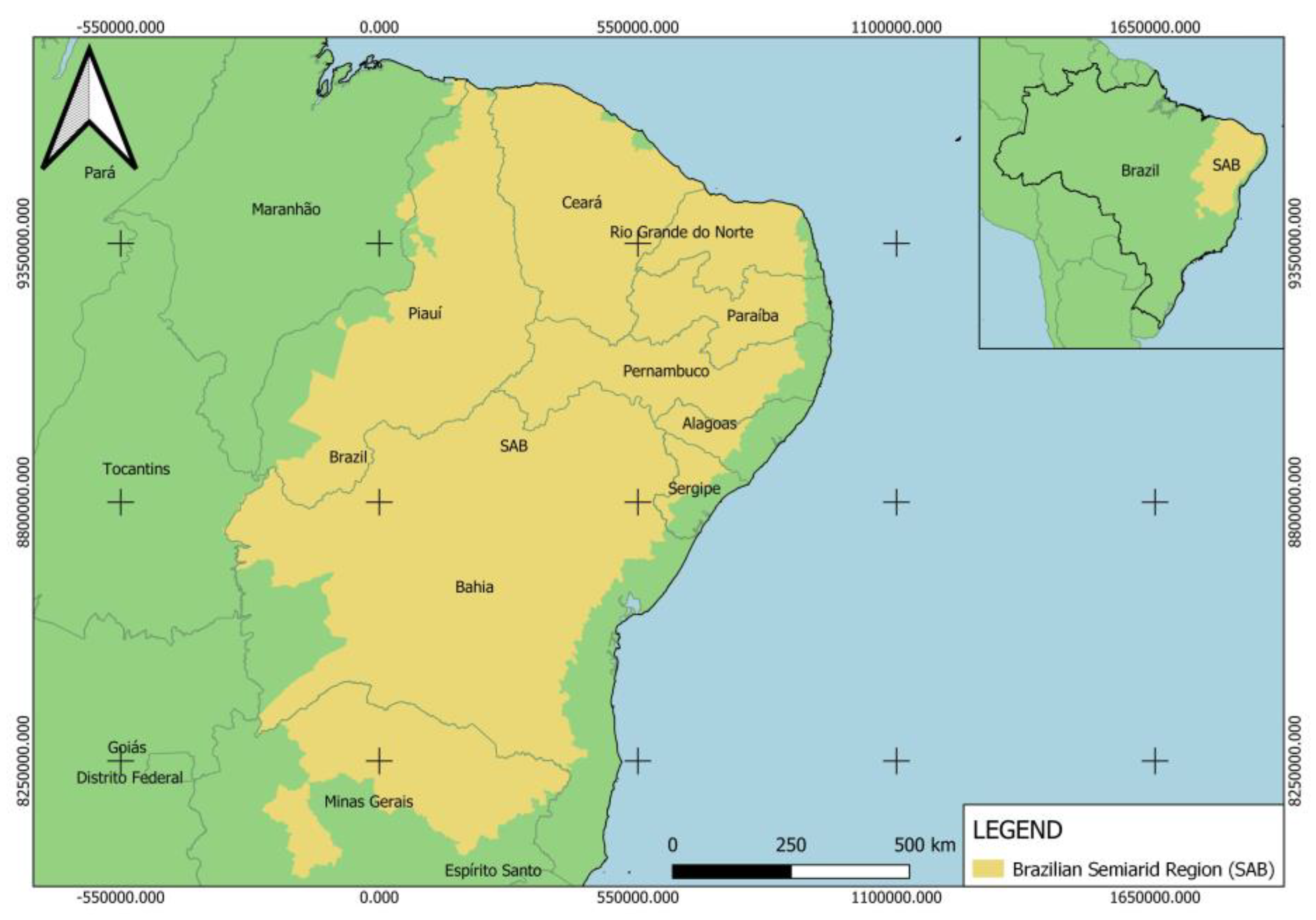
In Brazil, drought is characterized by its wide spatial coverage and recurrence in the Brazilian Semiarid Region (Semiárido Brasileiro—SAB), mainly due to its hydric vulnerability [67]. Approximately 28 million people live in this region [68], making it the most densely populated dry region in the world [69]. The Brazilian Semiarid Region is an area bounded by the Superintendence for the Development of the Northeast (Superintendência de Desenvolvimento do Nordeste—SUDENE) concerning precipitation and aridity conditions that currently includes 1262 municipalities (Figure 2).
In the SAB, there are diffuse communities and farmers with no reliable access to water and who, therefore, depend on mechanisms to address water scarcity. For those, drought management has been undertaken through measures such as rain-fed water cisterns construction, well drilling and recovery, dam and pumping station construction, as well as social safety programs such as Operação Carro Pipa (OCP), Bolsa Estiagem, and Garantia Safra [10]. The Brazilian Army has taken part in two of these programs: Operação Carro-Pipa and Operação Semiárido.
Operação Carro-Pipa was created in 2012, a technical and financial cooperation between the Ministry of National Integration and the Ministry of Defense [70]. This program aims to complement the water distribution carried out by the municipalities in the SAB. It was a temporary measure that is now carried out continuously due to the severity of the drought in this region as well as the growing number of municipalities included in the program. The Army’s role refers to the planning, coordination, and supervision of the activities carried out by outsourcing water trucks that involve search, transport, disinfection, and distribution of drinking water [71].
Operação Semiárido was also a partnership between the Ministry of National Integration and the Ministry of Defense. Its main objective was to reduce the dependence of SAB communities on water from water trucks as well as to increase water subsistence in this region. To accomplish that, still in the planning phase, a study was conducted using the database of Operação Carro Pipa to define the well locations that would benefit the most populous and farthest municipalities within the distribution logistics of water. This program has covered seven states in the Northeast Region, serving 80 municipalities in the semiarid region, and directly benefiting almost 69,000 people. The total cost of the program was BRL 15.7 million for approximately three years of duration; however, it is estimated that it can generate savings of BRL 6 million per year in the Operação Carro Pipa. During the existence of the program, 593 wells were drilled (302 of which contained water) and 23 reverse osmosis systems were also installed for the treatment of brackish water [72].
Policies for drought mitigation have evolved and now there is the understanding that the existing approaches are not mutually exclusive and can be integrated, resulting in a synergy to respond to the unpredictability of the drought. For example, rain-fed cisterns which should only store rainwater are being used for the storage of water from perennial water systems or artesian wells, transported by water trucks [16].

4.1. Data Collection

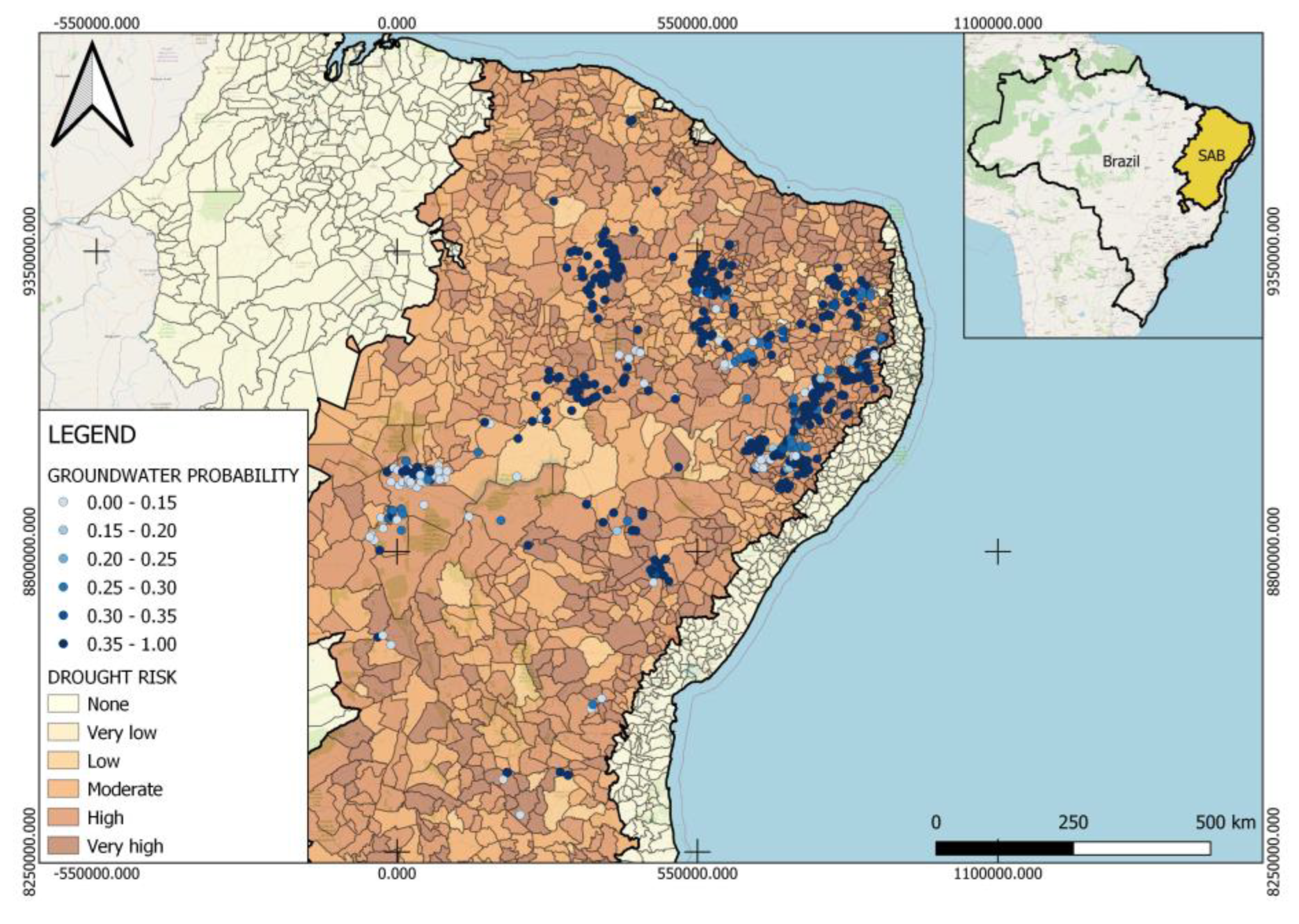
The database of the OCP with 739 demand points was used to validate our model. These points are in the Brazilian Semiarid Region, which involves 170 municipalities in the Northeast Region of Brazil; more specifically, the states of Alagoas, Pernambuco, Paraíba, Bahia, Ceará, Piauí, and Rio Grande do Norte (Figure 3).
From the OCP database, it was possible to obtain the exact location of the demand points (cisterns), as well as the number of people served by each cistern. From this number, the demand required by each point was calculated using the established value of 20 L per person per day of water [73]. We worked with an annual demand, having in mind that droughts usually happen annually. The distance matrix was obtained through the Google Map Distance Matrix API and, for the maximum coverage distance, we considered the value of 250 km based on the distances performed by the OCP.
Physical data such as lithology, drainage density, fracture density, and fracture proximity were extracted from files in shapefile format obtained from the Mineral Resources Research Company (Companhia de Pesquisa de Recursos Minerais—CPRM) and processed using QGIS software. These data were collected to determine the probabilities of groundwater occurrence through the regression formula proposed by [27].
Furthermore, from the database of the 1st Construction Engineering Battalion (1º Batalhão de Engenharia de Construção—1º BEC), a military unit employed in the Operação Semiárido and located in Caicó, Rio Grande do Norte, we estimated the average flow rate of an artesian well at 10 m3/h. Thus, considering an eight-hour working day, it was possible to obtain the annual capacity of the wells. The setup cost of an artesian well was estimated at USD 3596.70 according to this database, disregarding the cases of brackish water, which would imply a higher setup cost since it requires a reverse osmosis system.
Regarding transport costs, we used the calculation method applied in OCP. According to this method, transport is paid based on a transport unit of measure (TUM) calculated through Equation (27) where Ca is the capacity of water trucks, Di is the distance between the water supply and the demand point, Nt represents the number of trips, and Mi is a multiplier index related to road condition. The values for this index are provided in [74] and, in our case study, we considered all roads to be 100% unpaved road ( M i = 0.79 ) and the capacity of water trucks equals 20 m³, since these are the trucks most used in water distribution [73].
T U M = C a × D i × N t × M i
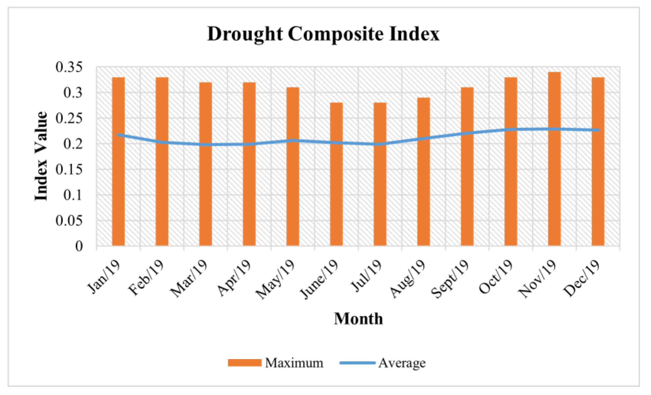
The drought composite index values for each municipality were taken from the DRAI platform, available at https://drai.live/ (accessed on 15 May 2023), an outcome from the work of [23]. The author of [23] categorized the risk index as follows: none ( 0.00 I R i < 0.15 ); very low ( 0.15 I R i < 0.20 ); low ( 0.20 I R i < 0.25 ); moderate ( 0.25 I R i < 0.30 ); high ( 0.30 I R i < 0.35 ); and very high ( 0.35 I R i < 1.00 ). The chosen year for the analysis was 2019 since it is the most current data available on the platform. We also evaluated the values of the indices for each month to determine what month to use in our analysis. November presented the highest indices in that year, characterizing a drier period, and then we decided to use it for safety’s sake. Figure 4 presents the index values for the year 2019.
The following parameters require some definitions from the decision maker. We adopted the budget limit to setup costs ( S c ) the value of USD 710,948.09. This value was obtained by multiplying the total number of wells drilled in Operação Semiárido by its setup cost and then dividing by the duration of the operation. For the budget limit for transportation costs T c , we used the known annual costs of distributing water to the same demand points considered in this article from the database of Operação Carro-Pipa, an estimated amount of USD 12,908,299.04.
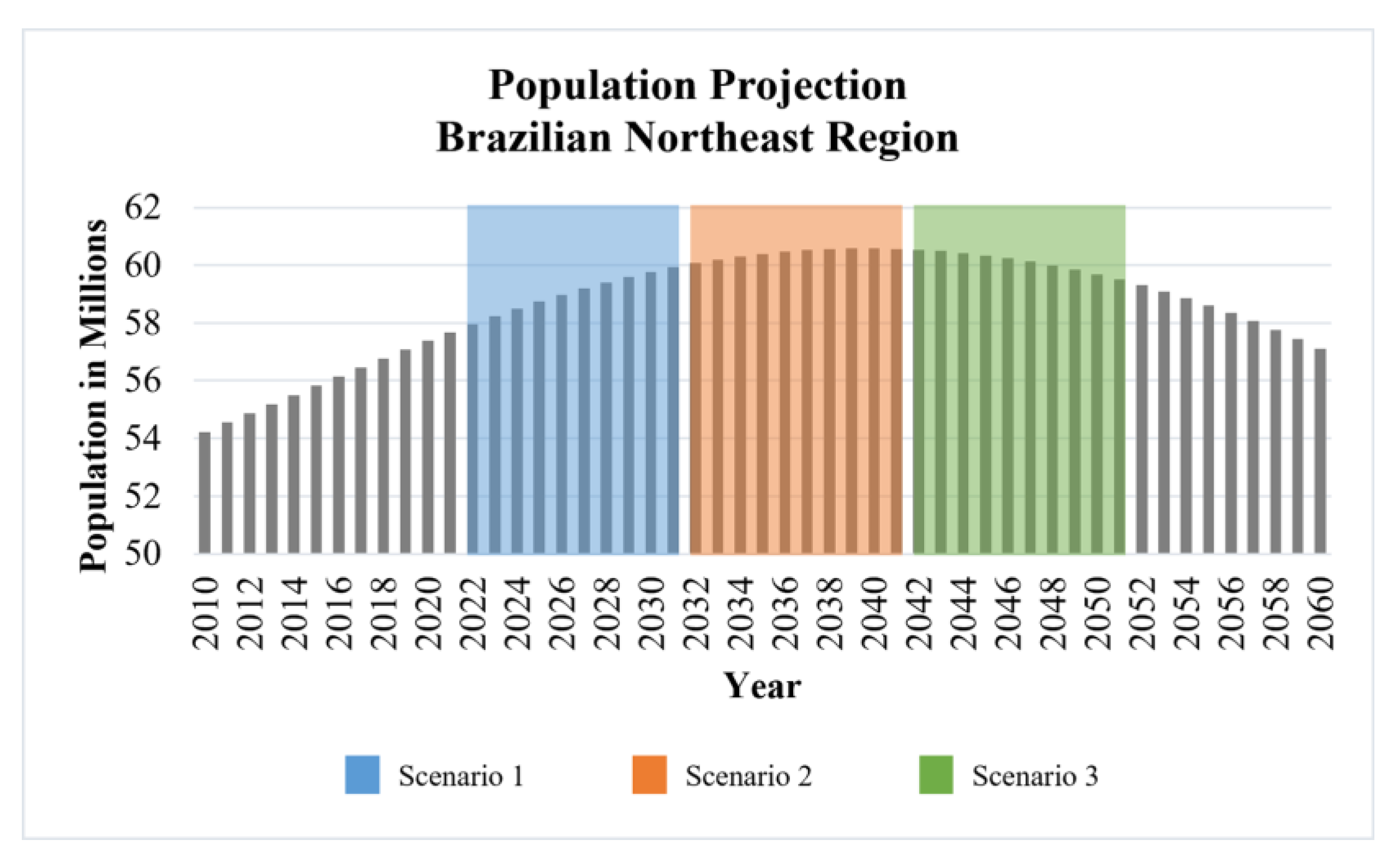
For the robust approach considering demand uncertainty, we work with three scenarios, each one representing a different rate of growth. The scenarios were chosen from the analysis of the population projection graph of the Brazilian Northeast Region (Figure 5), which was based on [75], starting in 2022 and considering periods of 10 years of duration, the same period as the demographic census. Thus, the periods selected were 2022–2031, 2032–2041, and 2042–2051. The choice of these ranges was based on the purpose of obtaining growth rates that would translate the three different trends observed in the graph: upward (increasing demand), nearly constant (practically unchanged demand), and downward (decreasing demand). The growth rates calculated for these periods are presented in Table 3.

4.2. Results

In this section, we present the computational results and analyze the behavior of the proposed models. As mentioned in Section 3.4, we solve the problem using the software AIMMS on a Core i7 with 8 GB of RAM under the Windows 64-bit environment. The proposed models and case study parameters were inputted into AIMMS. First, we ran the deterministic model, presented in Section 3.2, for each of the demand scenarios, including the current demand. Then, we ran the same model, but this time removing the drought risk index from the objective function presented in Equation (2). The mixed-integer programming (MIP) problem was solved by CPLEX 22.1, including the creation of 547,600 variables, of which 546,860 are integers, and the optimal solutions were obtained in an average time of 5033.83 s. Table 4 and Table 5 show the results of both executions.
From the table above, it is possible to note that the value of the objective function decreases as demand increases, as expected, since demand is the parameter that has the greatest influence on the result. Scenario 1, which predicts the greatest demand, is the one that has the highest value for the objective function (maximization), presenting the greatest social benefit since it meets a greater demand. It can also be noted that this scenario was the one with the largest number of wells located to meet all the demand and, consequently, it presents the lowest water transportation cost due to the reduction of well–cistern distances. In general, all demand points were met in all scenarios.
Table 5 shows the benefit of considering the composite drought risk index as a model parameter, aiming to prioritize the communities most affected by drought. The model performs this prioritization by allocating wells located at points with higher probability of productive wells to these communities, thus increasing the probability of meeting their demands. For the optimization that considers the drought risk index, the average probability of groundwater of the wells allocated to each cistern follows the risk classification of the community where it is located, so that communities with higher risk of drought are allocated to wells located in places with higher water probability. On the other hand, the optimization that does not consider the drought risk index does not follow the same logic.
For the robust optimization, we considered that each scenario presented in the previous section has a probability of occurrence, forming a probability vector. Different probability vectors were considered for the experiments, as follows.
  • Experiment 1 (equiprobable scenarios): r s = 1 3 , 1 3 , 1 3
  • Experiment 2 (Scenario 1 most likely): r s = 1 2 , 1 4 , 1 4
  • Experiment 3 (Scenario 2 most likely): r s = 1 4 , 1 2 , 1 4
  • Experiment 4 (Scenario 3 most likely): r s = 1 4 , 1 4 , 1 2
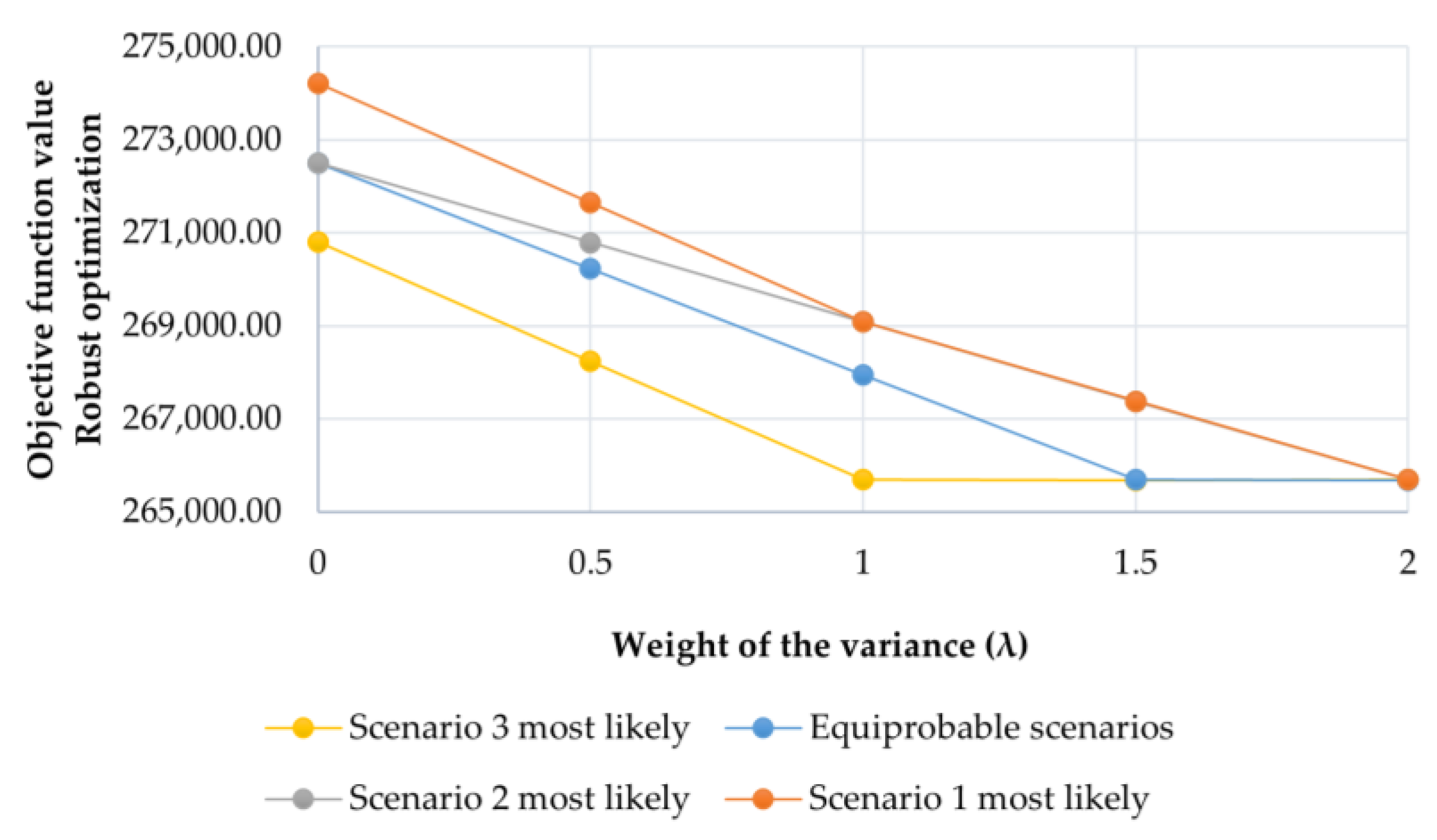
Moreover, the parameter λ was varied from 0 to 2. Keeping in mind that it represents the weight assigned to the variance of the solution, it can be understood as the decision maker’s risk aversion. The mixed-integer programming (MIP) problem was solved by CPLEX 22.1, including the creation of 1,641,326 variables, of which 1,639,102 are integers, and the optimal solutions were obtained in an average time of 6,378.84 s. Figure 6 presents the variation of the optimal solution of the robust model (Section 3.3) for different degrees of risk aversion. As expected, the objective function value worsens as the degree of risk aversion increases, which represents more conservative solutions.
For the sake of brevity, we decided to present the analysis of the results obtained for the case of equiprobable scenarios. However, the same analyses can be repeated for the other scenarios. From the graph analysis (Figure 6), in comparison to the values in Table 4, we can note that, as expected, robust optimization presents a worse result in terms of objective function compared to the deterministic model solution for the higher demand scenarios (Scenarios 1 and 2). For example, considering λ = 0.5 for the experiment in which scenario 1 is the most likely, the value of the robust solution is equal to 271,650.27 while the solution of the deterministic model of Scenario 1 generated a solution equal to 279,333.51. This means that the other scenarios are influencing the robust solution which seeks a near-optimal solution for all scenarios.
Figure 6 also shows that the value of the objective function tends to stabilize after a certain value of λ. For example, in the case of equiprobable scenarios, after λ = 1.5 the value of the objective function tends to remain constant, suffering little significant variations. This can also be seen in Table 6, which shows the variances of the solutions obtained for each scenario in the robust optimization for equiprobable scenarios depending on the value of λ chosen. This is a very relevant aspect for the decision maker when it comes to choosing the value of this parameter and to the advantage or disadvantage of investing in more conservative solutions.
This conservatism regarding the solution has some consequences. As λ increases, some demand points may no longer be met in some scenarios, specifically Scenarios 1 and 2, which have higher demands, as shown in Table 7. Starting at λ = 1.5 , some points are no longer served in Scenarios 1 and 2. Scenario 3, with lower demand, is not affected, with all points being served for any value of λ.
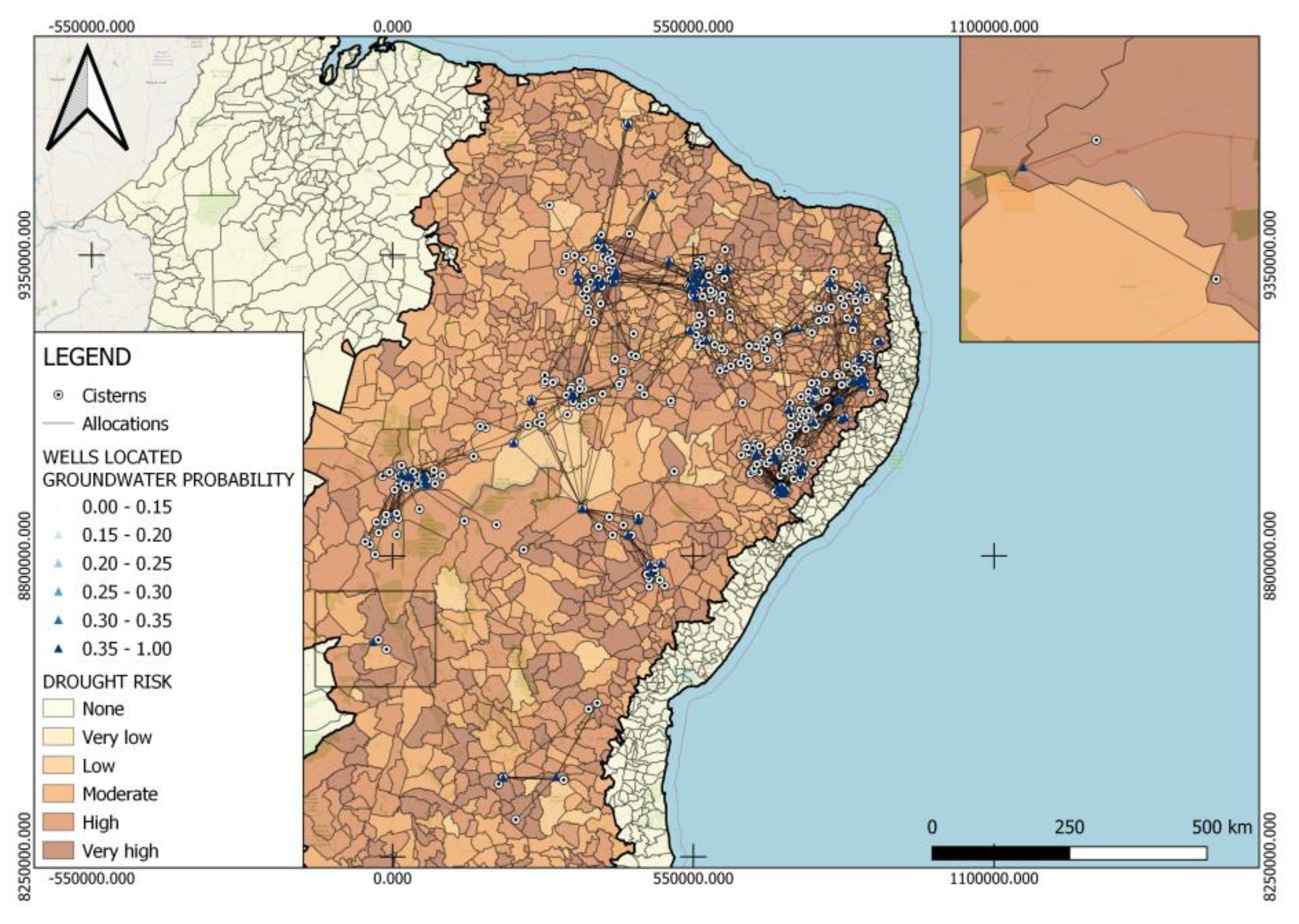
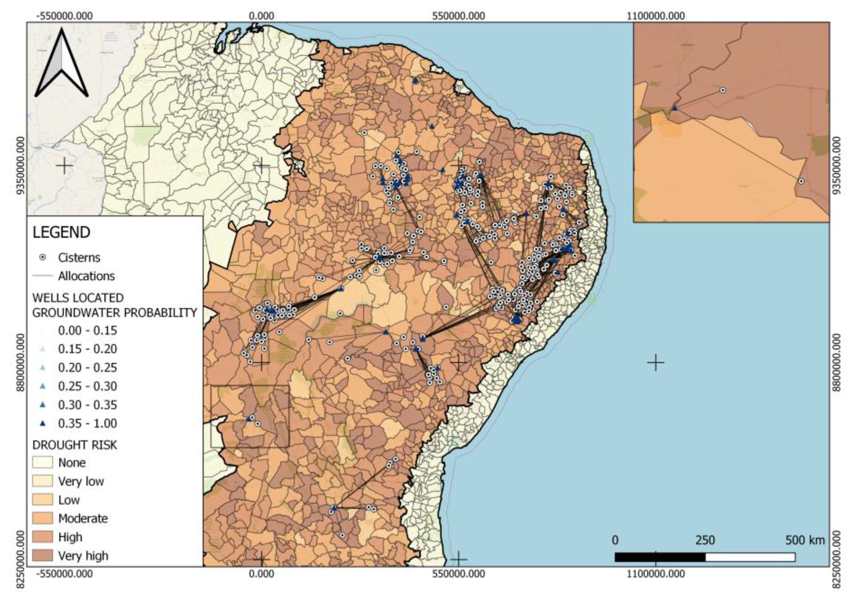
Figure 7, Figure 8 and Figure 9 show the allocations returned by the model for the robust optimization in the case of equiprobable scenarios and considering λ = 1.5, for each scenario. It is relevant to reiterate that the wells located do not change, for it is a decision that is not affected by the uncertainty. However, the allocations between the cisterns and these wells do change as the demand scenarios change.
A common measure in planning under uncertainty is worst-case optimization. Table 8 presents a comparison between the results obtained in the deterministic and robust optimizations for different experiments. The deterministic result analyzed considers the optimization for the worst scenario, which has the highest demand (Scenario 1), and calculates the expected value of this plan considering the probability vectors for the different scenarios. Note that the robust optimization returned a better expected value, considering all scenarios. This shows the advantage of the robust approach over the deterministic one under uncertainty.

4.3. Discussion and Managerial Insights

The models proposed in this paper deal with costs as constraints, considering that humanitarian operations are usually budget constrained. Nevertheless, managers can play with the values of the parameters S c and T c in order to achieve more economically interesting values.
The objective function aims to maximize the demand coverage while prioritizing the communities located in areas with higher drought risk and, at the same time, maximizing the probability of obtaining productive wells. Since the budget is not always sufficient to attend to all the demand points, our models serve as a decision support tool to assist in the choice of which points to attend based on drought risk. Moreover, by attempting to increase water prospecting success rates, the models also provide financial savings contributing to a reduction in the number of unproductive wells.
Finally, our model can deal with uncertainties in demand, allowing long-term planning and the solution adjustment according to the occurrence of the different demand scenarios. In addition, the manager can assign preference in terms of risk aversion degree, opting or not for more conservative solutions through the parameter λ.

5. Conclusions and Recommendations

In this paper, we proposed a deterministic and a robust stochastic programming model to optimize the location of artesian wells aiming both to reach success in obtaining groundwater and to prioritize the most vulnerable communities. Our model consists of two stages; the first stage determines the location of the artesian wells and the second stage determines well–cistern assignments. In our model, water demand is subject to uncertainty. To demonstrate the effectiveness of the robust model, a case study based on a program called Operação Carro Pipa that takes place in the Brazilian semiarid region is presented. Sensitivity analysis is also performed to show the advantage of a robust solution under uncertainty.
The results of our case study show that, even though robust optimization returns a less attractive value in terms of the objective function for a specific scenario, the robust solution is better than the deterministic one when we consider the expected value that they return, considering all scenarios for the uncertain parameter. Because both the model and the computed results are obtained from a set of real data, we have confidence in the practicability of these conclusions for dealing with uncertain scenarios. Moreover, robust results can also vary depending on decision makers’ risk aversion, represented in the model by the weight attributed to solution variance. Therefore, decision makers involved in relief planning can benefit from our model.
In addition to the contribution arising from the use of a robust approach, this paper presents a novel contribution regarding the use of a parameter that can represent the probability of obtaining productive wells, considering geological characteristics for this purpose, and a composite drought risk index which takes into account the threat of a drought event in a given location and the vulnerability of the community there, as a way to prioritize populations in areas with a higher risk of drought. This causes the model to shift from just focusing on costs to also focusing on the physical aspects of the candidate well sites and social aspects of drought-affected communities, thus allowing the best use of the scarce resources available for this purpose.
Therefore, we are confident that this research can contribute to the sustainability of communities in drought regions by guaranteeing water supply, which is crucial for economic activities and the subsistence of local people. Furthermore, these aspects are extremely important in the light of the expected increase in the occurrence of natural disasters in the coming years, intensified by climate change and population growth. In this regard, decision support tools, such as the one presented in this work, are desirable since they can significantly assist disaster management, helping leaders and planners in drought areas to establish the best coping strategies.
Therefore, we make the following relevant suggestions for further research:
  • A Multi-Criteria Decision Making (MCDM) method, such as AHP (Analytic Hierarchy Process), could be applied to set weights for the multiple objectives. Then, instead of considering transportation and setup costs as constraints, one could use them to compose the objective function;
  • To deepen the present study, it would be relevant to consider other uncertain parameters in the robust model, such as precipitation indices and well’s flow rate;
  • It would be interesting to improve the estimate of the probabilities concerning real scenarios once the robust approach highly depends on it.

Author Contributions

Conceptualization, O.S.d.S.J., R.A.d.M.B., and Y.E.M.V.; investigation, Y.E.M.V.; methodology, D.R.d.C.N., O.S.d.S.J., and R.A.d.M.B.; validation, D.R.d.C.N., O.S.d.S.J., and R.A.d.M.B.; writing—original draft preparation, D.R.d.C.N.; writing—review and editing, D.R.d.C.N., O.S.d.S.J., and R.A.d.M.B. All authors have read and agreed to the published version of the manuscript.

Funding

This research received no external funding.

Institutional Review Board Statement

Not applicable.

Informed Consent Statement

Not applicable.

Data Availability Statement

Data will be available on request.

Conflicts of Interest

The authors declare no conflict of interest.

References

  1. Ortega-Gaucin, D.; Pérez, M.L.; Cortés, F.A. Drought risk management in Mexico: Progress and challenges. Int. J. Saf. Secur. Eng. 2016, 6, 161–170. [Google Scholar] [CrossRef] [Green Version]
  2. Cunha, A.P.M.; do, A.; Marchezini, V.; Lindoso, D.P.; Saito, S.M.; Alvalá, R.C.; dos, S. The challenges of Consolidation of a Drought-Related Disaster Risk Warning System to Brazil. Sustain. Debate 2019, 10, 43–76. [Google Scholar] [CrossRef] [Green Version]
  3. Van Wassenhove, L. Blackett memorial lecturet humanitarian aid logistics: Supply chain. J. Oper. Res. Soc. 2006, 57, 475–489. [Google Scholar] [CrossRef]
  4. Pelling, M.; Özerdem, A.; Barakat, S. The macro-economic impact of disasters. Prog. Dev. Stud. 2002, 2, 283–305. [Google Scholar] [CrossRef] [Green Version]
  5. Hao, Z.; Hao, F.; Singh, V.P.; Ouyang, W.; Cheng, H. An integrated package for drought monitoring, prediction and analysis to aid drought modeling and assessment. Environ. Model. Softw. 2017, 91, 199–209. [Google Scholar] [CrossRef]
  6. CEPED UFSC (Centro Universitário de Estudos e Pesquisas sobre Desastres—Universidade Federal de Santa Catarina). Atlas Brasileiro de Desastres Naturais 1991 a 2010. Volume Brasil, Volume Pará, Volume Amapá, Florianópolis, 2012. Available online: https://www.ceped.ufsc.br/wp-content/uploads/2012/01/AMAZONAS_mioloWEB.pdf (accessed on 8 September 2022).
  7. Sena, A.; Barcellos, C.; Freitas, C.; Corvalan, C. Managing the health impacts of drought in Brazil. Int. J. Environ. Res. Public Health 2014, 11, 10737–10751. [Google Scholar] [CrossRef] [Green Version]
  8. Água Para Todos. Available online: https://antigo.mdr.gov.br/dadosabertos/317-secretaria-nacional-de-programas-urbanos/agua-para-todos/6076-agua-para-todos (accessed on 8 September 2022).
  9. Brito, S.S.B.; Cunha, A.P.M.; Cunningham, C.C.; Alvalá, R.C.; Marengo, J.A.; Carvalho, M.A. Frequency, duration and severity of drought in the Semiarid Northeast Brazil region. Int. J. Climatol. 2018, 38, 517–529. [Google Scholar] [CrossRef]
  10. Gutiérrez, A.P.A.; Engle, N.L.; De Nys, E.; Molejón, C.; Martins, E.S. Drought preparedness in Brazil. Weather and Clim. Extrem. 2014, 3, 95–106. [Google Scholar] [CrossRef] [Green Version]
  11. Nam, W.H.; Hayes, M.J.; Svoboda, M.D.; Tadesse, T.; Wilhite, D.A. Drought hazard assessment in the context of climate change for South Korea. Agric. Water Manag. 2015, 160, 106–117. [Google Scholar] [CrossRef]
  12. Akgün, İ.; Gümüşbuğa, F.; Tansel, B. Risk based facility location by using fault tree analysis in disaster management. Omega 2015, 52, 168–179. [Google Scholar] [CrossRef]
  13. Coppola, D.P. Introduction to International Disaster Management; Elsevier: Amsterdam, The Netherlands, 2007. [Google Scholar]
  14. Boonmee, C.; Arimura, M.; Asada, T. Facility location optimization model for emergency humanitarian logistics. Int. J. Disaster Risk Reduct. 2017, 24, 485–498. [Google Scholar] [CrossRef]
  15. Owen, S.H.; Daskin, M.S. Strategic facility location: A review. Eur. J. Oper. Res. 1998, 111, 423–447. [Google Scholar] [CrossRef]
  16. Machado, T.T.V.; Dias, J.T.; Silva, T.C.D. Evolução e avaliação das políticas públicas para a atenuação dos efeitos da seca no semiárido brasileiro. Gaia Sci. 2017, 11, 84–103. [Google Scholar] [CrossRef] [Green Version]
  17. Nag, S.K.; Kundu, A. Delineation of groundwater potential zones in hard rock terrain in Kashipur block, Purulia district, West Bengal, using geospatial techniques. Int. J. Waste Resour. 2016, 6, 1000201. [Google Scholar] [CrossRef]
  18. Limaye, S.D. Groundwater Development in Hard Rocks. Groundwater 2002, 2. Available online: http://www.eolss.net/Sample-Chapters/C07/E2-09-05-05.pdf (accessed on 8 September 2022).
  19. Singh, K.K.K.; Bharti, A.K.; Pal, S.K.; Prakash, A.; Kumar, R.; Singh, P.K. Delineation of fracture zone for groundwater using combined inversion technique. Environ. Earth Sci. 2019, 78, 1–12. [Google Scholar] [CrossRef]
  20. Zhang, D.D.; Yan, D.H.; Lu, F.; Wang, Y.C.; Feng, J. Copula-based risk assessment of drought in Yunnan province, China. Nat. Hazards 2015, 75, 2199–2220. [Google Scholar] [CrossRef]
  21. Wilhite, D.A. Drought as a natural hazard: Concepts and definitions. In Drought: A Global Assessment; Routledge: London, UK, 2000; Volume 1, pp. 3–18. [Google Scholar]
  22. González Tánago, I.; Urquijo, J.; Blauhut, V.; Villarroya, F.; De Stefano, L. Learning from experience: A systematic review of assessments of vulnerability to drought. Nat. Hazards 2016, 80, 951–973. [Google Scholar] [CrossRef]
  23. Bravo, R.Z.B. Monitoramento e alerta de secas no Brasil: Nova abordagem baseada em um índice de risco. Doctoral Thesis, Pontifícia Universidade Católica do Rio de Janeiro, Rio de Janeiro, Brazil, 2021. [Google Scholar]
  24. Habib, M.S.; Lee, Y.H.; Memon, M.S. Mathematical models in humanitarian supply chain management: A systematic literature review. Math. Probl. Eng. 2016, 2016, 3212095. [Google Scholar] [CrossRef] [Green Version]
  25. Zokaee, S.; Bozorgi-Amiri, A.; Sadjadi, S.J. A robust optimization model for humanitarian relief chain design under uncertainty. Appl. Math. Model. 2016, 40, 7996–8016. [Google Scholar] [CrossRef] [Green Version]
  26. Yu, C.S.; Li, H.L. A robust optimization model for stochastic logistic problems. Int. J. Prod. Econ. 2000, 64, 385–397. [Google Scholar] [CrossRef]
  27. Vieira, Y.E.M.; Bandeira, R.A.M.; da Silva Junior, O.S. Application of a Logit Model for Water well site location in fractured-bedrock aquifers in northeastern Brazil. Int. J. Innov. Educ. Res. 2022, 10, 33–52. [Google Scholar] [CrossRef]
  28. Laporte, G.; Nickel, S.; Saldanha-da-Gama, F. Introduction to location science. In Location Science; Springer: Berlin/Heidelberg, Germany, 2019; pp. 1–21. [Google Scholar]
  29. Hakimi, S.L. Optimum locations of switching centers and the absolute centers and medians of a graph. Oper. Res. 1964, 12, 450–459. [Google Scholar] [CrossRef]
  30. Hakimi, S.L. Optimum distribution of switching centers in a communication network and some related graph theoretic problems. Oper. Res. 1965, 13, 462–475. [Google Scholar] [CrossRef]
  31. Toregas, C.; Swain, R.; ReVelle, C.; Bergman, L. The location of emergency service facilities. Oper. Res. 1971, 19, 1363–1373. [Google Scholar] [CrossRef]
  32. Church, R.; ReVelle, C. The maximal covering location problem. Pap. Reg. Sci. Assoc. 1974, 32, 101–118. [Google Scholar] [CrossRef]
  33. Cornuejols, G.; Fisher, M.; Nemhauser, G.L. On the uncapacitated location problem. Ann. Discret. Math. 1977, 1, 163–177. [Google Scholar]
  34. Current, J.R.; Storbeck, J.E. Capacitated covering models. Environ. Plan. B Plan. Des. 1988, 15, 153–163. [Google Scholar] [CrossRef]
  35. Sankaran, J.K.; Raghavan, N.S. Locating and sizing plants for bottling propane in south India. Interfaces 1997, 27, 1–15. [Google Scholar] [CrossRef]
  36. Alp, O.; Erkut, E.; Drezner, Z. An efficient genetic algorithm for the p-median problem. Ann. Oper. Res. 2003, 122, 21–42. [Google Scholar] [CrossRef]
  37. Mladenović, N.; Labbé, M.; Hansen, P. Solving the p-center problem with tabu search and variable neighborhood search. Netw. Int. J. 2003, 42, 48–64. [Google Scholar] [CrossRef] [Green Version]
  38. Daskin, M.S. SITATION Facility Location Software; Department of Industrial Engineering and Management Sciences, Northwestern University: Evanston, IL, USA, 2002. [Google Scholar]
  39. Muñoz-Márquez, M. Orloca: Operations Research LOCational Analysis Models; Departamento de Matematicas, Departamento de Estadistica e Investigacion Operativa, Universidad de Cadiz: Cadiz, Spain, 2008. [Google Scholar]
  40. Kalcsics, J.; Butsch, A.; Jürgens, R. Library of Location Algorithms (LoLA); Institute of Operations Research, Karlsruhe Institute of Technology: Karlsruhe, Germany, 2011. [Google Scholar]
  41. Erdoğan, G.; Stylianou, N.; Vasilakis, C. An open source decision support system for facility location analysis. Decis. Support Syst. 2019, 125, 113116. [Google Scholar] [CrossRef]
  42. Lin, Y.; Jia, H.; Yang, Y.; Tian, G.; Tao, F.; Ling, L. An improved artificial bee colony for facility location allocation problem of end-of-life vehicles recovery network. J. Clean. Prod. 2018, 205, 134–144. [Google Scholar] [CrossRef]
  43. Aras, N.; Bilge, Ü. Robust supply chain network design with multi-products for a company in the food sector. Appl. Math. Model. 2018, 60, 526–539. [Google Scholar] [CrossRef]
  44. Jabbarzadeh, A.; Haughton, M.; Khosrojerdi, A. Closed-loop supply chain network design under disruption risks: A robust approach with real world application. Comput. Ind. Eng. 2018, 116, 178–191. [Google Scholar] [CrossRef]
  45. Ghahremani-Nahr, J.; Kian, R.; Sabet, E. A robust fuzzy mathematical programming model for the closed-loop supply chain network design and a whale optimization solution algorithm. Expert Syst. Appl. 2019, 116, 454–471. [Google Scholar] [CrossRef] [Green Version]
  46. Saedinia, R.; Vahdani, B.; Etebari, F.; Nadjafi, B.A. Robust gasoline closed loop supply chain design with redistricting, service sharing and intra-district service transfer. Transp. Res. Part E Logist. Transp. Rev. 2019, 123, 121–141. [Google Scholar] [CrossRef]
  47. Yu, H.; Sun, X.; Solvang, W.D.; Laporte, G.; Lee, C.K.M. A stochastic network design problem for hazardous waste management. J. Clean. Prod. 2020, 277, 123566. [Google Scholar] [CrossRef]
  48. Mohammed, A.; Wang, Q. Multi-criteria optimization for a cost-effective design of an RFID-based meat supply chain. Br. Food J. 2017, 119, 676–689. [Google Scholar] [CrossRef] [Green Version]
  49. Mohammed, A.; Wang, Q.; Li, X. A cost-effective decision-making algorithm for an RFID-enabled HMSC network design: A multi-objective approach. Ind. Manag. Data Syst. 2017, 117, 1782–1799. [Google Scholar] [CrossRef] [Green Version]
  50. Mogale, D.G.; Kumar, M.; Kumar, S.K.; Tiwari, M.K. Grain silo location-allocation problem with dwell time for optimization of food grain supply chain network. Transp. Res. Part E Logist. Transp. Rev. 2018, 111, 40–69. [Google Scholar] [CrossRef]
  51. Wang, L.; Shi, H.; Gan, L. Healthcare facility location-allocation optimization for China’s developing cities utilizing a multi-objective decision support approach. Sustainability 2018, 10, 4580. [Google Scholar] [CrossRef] [Green Version]
  52. Chen, Y.; Lai, Z. A Multi-Objective Optimization Approach for Emergency Medical Service Facilities Location-Allocation in Rural Areas. Risk Manag. Healthc. Policy 2022, 15, 473. [Google Scholar] [CrossRef] [PubMed]
  53. Ni, W.; Shu, J.; Song, M. Location and emergency inventory pre-positioning for disaster response operations: Min-max robust model and a case study of Yushu earthquake. Prod. Oper. Manag. 2018, 27, 160–183. [Google Scholar] [CrossRef]
  54. Paul, J.A.; Wang, X.J. Robust location-allocation network design for earthquake preparedness. Transp. Res. Part B: Methodol. 2019, 119, 139–155. [Google Scholar] [CrossRef]
  55. Yahyaei, M.; Bozorgi-Amiri, A. Robust reliable humanitarian relief network design: An integration of shelter and supply facility location. Ann. Oper. Res. 2019, 283, 897–916. [Google Scholar] [CrossRef]
  56. Maharjan, R.; Hanaoka, S. A credibility-based multi-objective temporary logistics hub location-allocation model for relief supply and distribution under uncertainty. Socio-Econ. Plan. Sci. 2020, 70, 100727. [Google Scholar] [CrossRef]
  57. Mohammadi, S.; Darestani, S.A.; Vahdani, B.; Alinezhad, A. A robust neutrosophic fuzzy-based approach to integrate reliable facility location and routing decisions for disaster relief under fairness and aftershocks concerns. Comput. Ind. Eng. 2020, 148, 106734. [Google Scholar] [CrossRef]
  58. Ribas, G.P. Modelo de programação estocástica para o planejamento estratégico da cadeia integrada de petróleo. Master’s Thesis, Pontifícia Universidade Católica do Rio de Janeiro, Rio de Janeiro, Brazil, 2008. [Google Scholar]
  59. Mulvey, J.M.; Vanderbei, R.J.; Zenios, S.A. Robust optimization of large-scale systems. Oper. Res. 1995, 43, 264–281. [Google Scholar] [CrossRef] [Green Version]
  60. Bozorgi-Amiri, A.; Jabalameli, M.S.; Mirzapour Al-e-Hashem, S.M.J. A multi-objective robust stochastic programming model for disaster relief logistics under uncertainty. OR Spectr. 2013, 35, 905–933. [Google Scholar] [CrossRef]
  61. Jabbarzadeh, A.; Fahimnia, B.; Seuring, S. Dynamic supply chain network design for the supply of blood in disasters: A robust model with real world application. Transp. Res. Part E Logist. Transp. Rev. 2014, 70, 225–244. [Google Scholar] [CrossRef]
  62. Cunha, M.D.C.; Antunes, A.P. On the efficient location of pumping facilities in an aquifer system. Int. Trans. Oper. Res. 1997, 4, 175–184. [Google Scholar] [CrossRef]
  63. Ferreira, J.; Cunha, M.C.; Vieira, J.; Monteiro, J.P. Optimized exploitation of aquifers: Application to the Querença-Silves aquifer system. Water Resour. Manag. 2009, 125, 3. [Google Scholar]
  64. Ng, T.L. Expanding Neighborhood Tabu Search for facility location problems in water infrastructure planning. In Proceedings of the 2014 IEEE International Conference on Systems, Man, and Cybernetics (SMC), San Diego, CA, USA, 5–8 October 2014; pp. 3851–3854. [Google Scholar]
  65. Roman, O.; Hoque, S.F.; Ford, L.; Salehin, M.; Alam, M.M.; Hope, R.; Hall, J.W. Optimizing rural drinking water supply infrastructure to account for spatial variations in groundwater quality and household welfare in coastal Bangladesh. Water Resour. Res. 2021, 57, e2021WR029621. [Google Scholar] [CrossRef]
  66. Bravo, R.Z.B.; Cunha, A.P.M.D.A.; Leiras, A.; Cyrino Oliveira, F.L. A new approach for a drought composite index. Nat. Hazards 2021, 108, 755–773. [Google Scholar] [CrossRef]
  67. Alvalá, R.; Cunha, A.P.; Brito, S.S.; Seluchi, M.E.; Marengo, J.A.; Moraes, O.L.; Carvalho, M.A. Drought monitoring in the Brazilian Semiarid region. An. Da Acad. Bras. De Ciências 2017, 91. [Google Scholar] [CrossRef] [Green Version]
  68. Silva, J.M.C.D.; Barbosa, L.C.F.; Leal, I.R.; Tabarelli, M. The Caatinga: Understanding the challenges. In Caatinga: The Largest Tropical Dry Forest Region in South America; Springer: Berlin/Heidelberg, Germany, 2017; pp. 3–19. [Google Scholar]
  69. Marengo, J.A. Vulnerabilidade, impactos e adaptação à mudança do clima no semiárido do Brasil. Parcer. Estratégicas 2008, 27, 149–175. [Google Scholar]
  70. Brasil, Inteministerial Ordinance n.1. Provides for the mutual technical and financial cooperation between the Ministries of National Integration and Defense to carry out complementary actions to support the distribution of drinking water to the populations affected by drought and drought in the semi-arid region of the Northeast and the night region of the States of Minas Gerais and Espírito Santo, called Operação Carro Pipa. Diário Oficial da União, 25 July 2012.
  71. Portal da Operação Carro Pipa. Available online: http://sedec.5cta.eb.mil.br/ (accessed on 8 September 2022).
  72. Defesanet. Available online: https://www.defesanet.com.br/aciso/noticia/34215/exercito-brasileiro-finaliza-a-entrega-de-mais-de-300-pocos-artesianos-no-semiarido-nordestino/#:~:text=O%20Ex%C3%A9rcito%20Brasileiro%20encerrou%2C%20no,Regi%C3%A3o%20Nordeste%20do%20nosso%20pa%C3%ADs (accessed on 8 September 2022).
  73. Vieira, Y.E.M.; Bandeira, R.A.M.; da Silva Junior, O.S. Multi-depot vehicle routing problem for large scale disaster relief in drought scenarios: The case of the brazilian northeast region. Int. J. Disaster Risk Reduct. 2021, 58, 102193. [Google Scholar] [CrossRef]
  74. CMNE (Comando Militar Do Nordeste). Ordem de Serviço Nr 008 de 17 de agosto de 2015. Regula a Participação do Comando Militar do Nordeste no Programa Emergencial de Distribuição de Água Potável no Semiárido Brasileiro—Operação Carro-Pipa. Available online: https://6rm.eb.mil.br/images/servicos/operacao_pipa/pdf/Anexo_G-Criterios_para_Calculo_dos_Valores.pdf (accessed on 8 September 2022).
  75. IBGE. Available online: https://www.ibge.gov.br/estatisticas/sociais/populacao/9109-projecao-da-populacao.html?=&t=resultados (accessed on 8 September 2022).
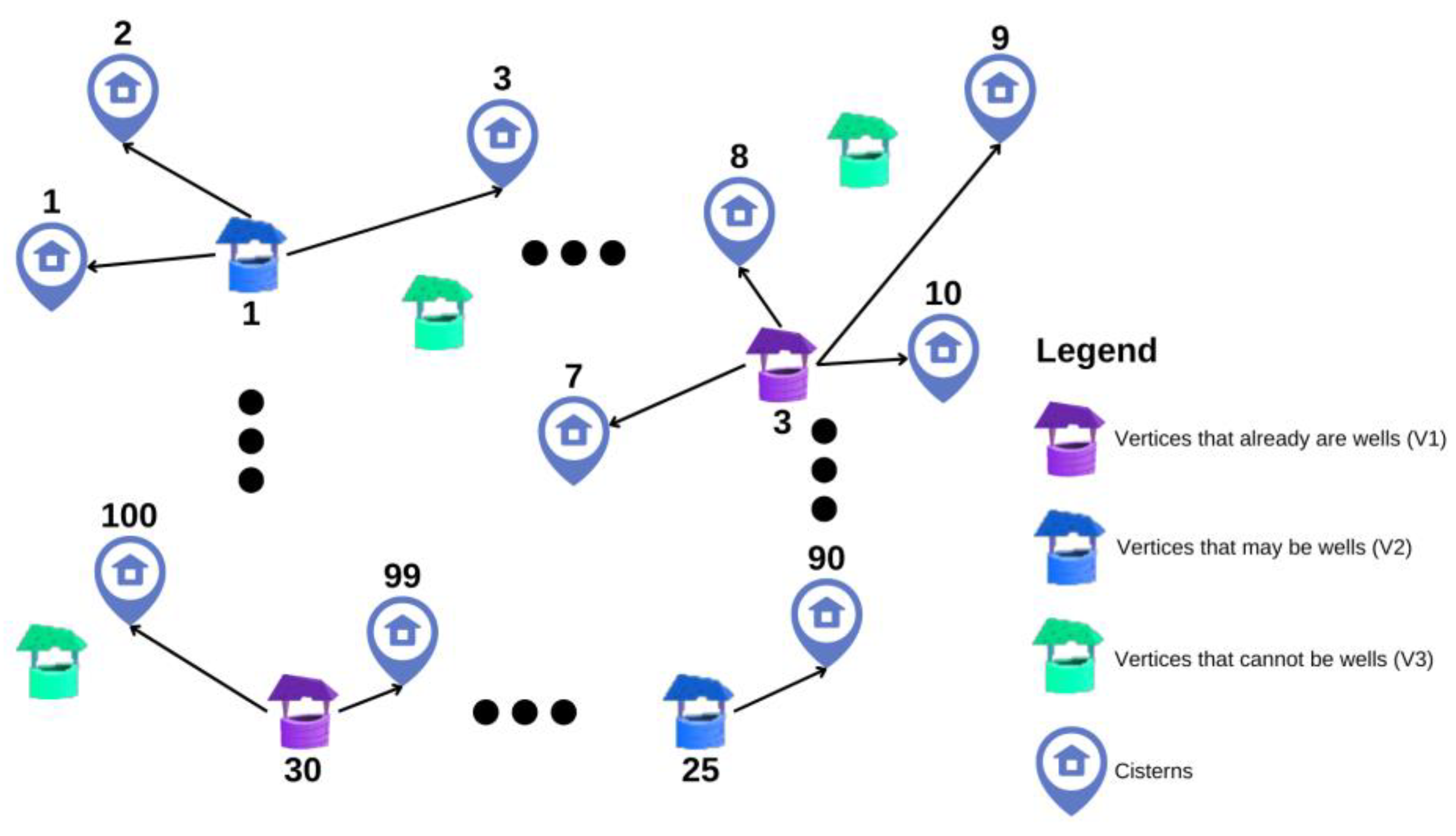
Figure 1. FLP for artesian wells to drought-affected populations.
Sustainability 15 10916 g001
Figure 2. Geographic limits of the Brazilian Semiarid Region.
Sustainability 15 10916 g002
Figure 3. OCP demand points used in the case study.
Sustainability 15 10916 g003
Figure 4. Drought composite index values for 2019.
Sustainability 15 10916 g004
Figure 5. Brazilian Northeast Region population projection.
Sustainability 15 10916 g005
Figure 6. Objective function value in robust optimization depending on the decision maker’s risk aversion.
Sustainability 15 10916 g006
Figure 7. Allocations returned for Scenario 1 in case of equiprobable scenarios for λ = 1.5.
Sustainability 15 10916 g007
Figure 8. Allocations returned for Scenario 2 in case of equiprobable scenarios for λ = 1.5.
Sustainability 15 10916 g008
Figure 9. Allocations returned for Scenario 3 in case of equiprobable scenarios for λ = 1.5.
Sustainability 15 10916 g009
Table 1. Description of the notations adopted in the deterministic model.
NotationDescription
G = V , A The complete digraph to represent the distribution network
V The set of all nodes (indexed by i and j)
V 1 The subset of V with the nodes that already are wells
V 2 The subset of V with the nodes that can be wells
V 3 The subset of V with the nodes that cannot be wells
p j The probability of occurrence of groundwater of node j
q i The water demand of node i
I R i The drought composite index of node i
s j The cost of installing a well in j
Q j The estimated capacity of a well located in j
δThe maximum service distance
d i j The distance between the nodes i and j
cThe average cost of transportation
S c The budget limit for well drilling
T c The budget limit for water distribution
x i j Equals 1 if node i is served by a facility in j, and 0 otherwise
y j Equals 1 if vertex j is going to locate a well, and 0 otherwise
Table 2. Description of the notations adopted in the robust model.
NotationDescription
SThe set of demand scenarios (indexed by s and s’)
r s The probability of occurrence of scenario s
q i s The water demand of node i in the scenario s
ΛThe weight assigned to the variance of the solution
x i j s Equals 1 if vertex i is served by a facility in j in scenario s, and 0 otherwise.
θ s The scenario-dependent auxiliary variable for the linearization of the model
Table 3. Growth rate for each scenario.
PeriodScenarioGrowth Rate
2022–203113.40%
2032–204120.84%
2042–20513−1.71%
Table 4. Deterministic optimization results for each demand scenario.
DemandObjective Function ValueNumber of Wells LocatedNumber of Points CoveredDemand CoveredTransportation Cost (US $)
Current270,263.641847391,149,830.3012,906,850.50
Scenario 1279,333.511927391,188,919.8612,512,629.46
Scenario 2272,500.211687391,159,475.6212,904,931.08
Scenario 3265,687.721687391,130,119.5512,907,292.52
Table 5. Comparison of the optimization results with and without prioritization through drought risk index (current demand).
RiskAverage Probability of Water Occurrence
Optimization with
Drought Risk Index
Optimization without
Drought Risk Index
High0.9955653440.981914234
Moderate0.9838963450.983896345
Low0.9780246540.979950119
Very low0.9630072830.983068566
Table 6. Variance of the robust optimization solutions for each scenario as a function of λ.
LambdaObjective FunctionVariance
Scenario 1Scenario 2Scenario 3
0.0279,333.19272,499.910.0279,333.19
0.5279,329.29272,495.610.5279,329.29
1.0279,293.16272,487.361.0279,293.16
1.5267,229.18268,764.411.5267,229.18
2.0265,684.02265,683.992.0265,684.02
Table 7. Number of points covered in each scenario in the robust optimization.
LambdaNumber of Points Covered
Scenario 1Scenario 2Scenario 3
0739739739
0.5739739739
1.0739739739
1.5716734739
2.0711734739
Table 8. Comparison between deterministic and robust optimization results.
ExperimentResultsDifference
Deterministic (Worst Scenario)Robust
Experiment 1
(Equiprobable scenarios)
268,847.64272,506.45−1.36%
Experiment 2
(Scenario 1 most likely)
268,787.90274,211.82−2.02%
Experiment 3
(Scenario 2 most likely)
269,739.64272,505.03−1.03%
Experiment 4
(Scenario 3 most likely)
268,015.36270,798.85−1.04%
Disclaimer/Publisher’s Note: The statements, opinions and data contained in all publications are solely those of the individual author(s) and contributor(s) and not of MDPI and/or the editor(s). MDPI and/or the editor(s) disclaim responsibility for any injury to people or property resulting from any ideas, methods, instructions or products referred to in the content.