Seasons Effects of Field Measurement of Near-Ground Wind Characteristics in a Complex Terrain Forested Region

Abstract

The wind characteristics of the atmospheric boundary layer in forested regions exhibit a significant complexity due to rugged terrain, seasonal climate variability, and seasonal growth of vegetation, which play a key role not only in designing optimal blades to gain better performance but also in assessing the structural response, and there is a paucity of research on such wind fields. Therefore, this paper investigates wind characteristics via on-site wind field measurement. The mean and fluctuating wind characteristics of the forested region in different seasons were analyzed based on the field measurement data. The results show that for the mean wind characteristics, the seasonally fitted exponents play a decisive role in characterizing the mean wind profile, while the season and temperature are the key factors affecting the mean wind direction in forested regions. For fluctuating wind characteristics, the seasonal power-law function can accurately characterize the turbulence intensity profile. Moreover, the ratio of the three turbulence intensity components is significantly affected by temperature and season, and the Von Kármán spectrum has better applicability in the cold and less canopy-disturbed winter than in the other three seasons. The proposed seasonally fitted parameters show better applicability in terms of vertical coherence.

1. Introduction

In recent decades, countries worldwide have been actively developing and using renewable energy, such as solar energy, geothermal energy, wind energy, ocean energy, biomass energy, etc. Wind energy is a clean, abundant, and widely distributed renewable energy. Meanwhile, the research and applications of wind power generation technology are becoming more and more mature [1,2,3]. However, traditional wind turbine locations are becoming increasingly saturated and forested regions are entering the public’s sights with their abundant natural resources [4]. The wind characteristics of the near-ground atmospheric boundary layer in forested regions are highly complex due to complex terrain, forest canopy, and seasonal factors. Moreover, Harbin has four distinct seasons: short spring and autumn, moderate summer, and long winter. The vegetation grows seasonally, with spring from late March to May, summer from June to August, autumn from September to mid-November, and winter from late November to mid-March [5,6,7]. Therefore, it is essential to accurately grasp the wind field characteristics of forested regions in different seasons to refinement study of the wind-sensitive structures’ wind-induced vibration response in forested regions (such as transmission towers and suspension ropeways and cable cars) to ensure the safety of forest infrastructure, and to develop forested regions for wind energy development and forest disaster prevention and mitigation [8,9,10].

In recent years, some scholars have gradually researched wind characteristics in forested regions. Field measurements, wind tunnel tests, and numerical simulations are three analytical methods to study wind characteristics in forested regions with complex terrain. In numerical simulations, Tamura [11] investigated vegetation’s effects on turbulent flow statistics on a 3D steep hill through large eddy simulations, elucidating the coherent flow structure at the top of the vegetation and the high turbulence intensity caused by the reduction of turbulence within the vegetation. Liu [12] modeled the vegetation canopy and successfully reproduced the complex terrain turbulence characteristics with vegetation cover by large eddy simulation. Based on CFD technology, Li [13] used a simplified porous media model to represent the tree model, simulated the wind field around trees in Class B typical standard wind terrain by adding additional source terms, and compared the simulation results with wind tunnel test data to verify the results. In terms of wind tunnel tests, Cao [14] studied the aerodynamic characteristics of three shrub trees suitable for dense green roofs through atmospheric boundary layer wind tunnel tests. This study showed that the drag coefficients of the trees were related to tree species and canopy porosity. Lee [15] used the PIV technique to quantitatively visualize the flow around a row of small white-shirted trees through a wind tunnel test to investigate the effect of windbreaks on the flow field structure and shading effects. The results show that a row of trees can effectively improve the flow field characteristics and shading effects in the study region. Li [16] investigated the relationship between tree wind load and wind speed under three arrangements of one plant, one row, and one column of trees by wind tunnel tests and also studied the flow field characteristics behind the trees under the first two arrangements. The study shows a power function relationship between tree wind load and wind speed, but different arrangements affect the tree wind load. Field measurements as the most direct and effective method among the three methods, some literature has peformed the following studies. Ma [17] studied the effectiveness of a shelterbelt with a non-uniform density distribution in weakening wind speed through field observations and then analyzed the wind-blocking effect of the shelterbelt. The results showed that the wind field variation characteristics on the windward and leeward sides of the shelterbelt were correlated with the density distribution of the shelterbelt. Santana [18] analyzed the vertical wind profile characteristics at six anemometer tower locations in a dense forest in the Amazon basin and showed that turbulence in the forest canopy structure could have a noted significant effect on the vertical wind profile below. Jiang [19,20] investigated the mean and fluctuating wind characteristics in a forest area during strong wind conditions by empirical field measurements. The results showed that the disturbance effect of trees caused the mean wind to deflect with height, and the disturbance effect of trees increased the intensity of turbulence within the canopy.

Many national specifications or standards propose wind field characteristic parameters for wind resistance design, such as the USA (ASCE 7–10) [21], Japan (AIJ-RLB-2004) [22], China (JTG/T3360-01) [23], ESDU [24], and Australia/New Zealand (AS/NSZ1170.2) [25]. However, specifications and standards are generally recommended for plains or coasts and cannot be fully relied upon for complex wind fields in the atmospheric boundary layer in forested regions of complex terrain with specified parameters. For example, for China (JTG/T3360-01) [23], the recommended ratio of longitudinal, lateral, and vertical turbulence intensities is 1:0.88:0.50, but some researchers [26,27,28] pointed out that the ratio of the three turbulence intensity components in mountainous regions is different from theirs. The turbulence spectrum and spatial coherence may also be different. Therefore, it is essential to conduct field measurements of turbulence fields in complex terrain.

Although a large number of studies have extensively reported observations of some complex terrain wind fields, these studies have generally been conducted for special weather in coastal regions (e.g., typhoons, downbursts, etc.) and complex terrain mountainous areas (e.g., bridge sites, valleys, etc.). Researchers have conducted studies on wind characteristics, such as wind profiles in forested regions, but no systematic studies and summaries have been conducted on the seasonal mean wind characteristics and fluctuating wind characteristics in forested regions. The purpose of this paper is to improve the understanding of mean wind profile, mean wind direction, turbulence intensity, turbulence spectrum, and vertical spatial coherence in complex terrain forested regions in different seasons and to provide suitable seasonally fitted parameters for the wind-resistant design of adaptation works in forested engineering sites. Therefore, long-term data of 20 m, 35 m, and 50 m of the flux tower were analyzed for the study. The subsequent contents of this paper are structured as follows: Section 2 describes the site selection, equipment, smoothness test, and data processing methods of the flux tower; Section 3 gives the wind field characteristics of the forested region in different seasons and compares them with current design specifications or empirical formulas; Section 4 summarizes the major conclusions of the field measurement study.

2. Equipment and Data Processing

The flux tower (N 45°24′31.5″, E 127°39′49.7″) is located in the Maoer Mountain Forest Ecosystem Research Station of Northeast Forestry University, Heilongjiang Province, Northeast China (Figure 1). Abundant forest resources surround the observation site, and the site’s climate is continental monsoon with a windy, dry spring, a warm and humid summer, and a dry and cold winter [29]. The wind observation system consists of five ultrasonic anemometers (Wind Master, GILL, Hampshire, UK), a CR6 data collector (Campbell, Logan, UT, USA), and a power supply system (Figure 2a). The ultrasonic anemometer wind speed measurement range is 0~45 m/s, the resolution is 0.01 m/s, the accuracy is 1.5 RMS@12 m/s, and the sampling frequency can reach 20 Hz or 32 Hz. Considering the low order inherent frequency of the structure of the infrastructure construction in complex terrain forested regions is usually less than 5 Hz, the output frequency of the ultrasonic anemometer is set to 10 Hz to meet the sampling law requirements. As shown in Figure 2b, five 3D ultrasonic anemometers were installed at 5 m, 10 m, 20 m, 35 m, and 50 m heights.

In the field wind monitoring process, the ultrasonic anemometer needs to continuously and uninterruptedly send ultrasonic waves to collect wind speed and wind direction data, in the collection process, the ultrasonic anemometer is sensitive to unfavorable weather conditions such as floating objects in the air or heavy precipitation, thunderstorms, etc., and data collection will be affected resulting in abnormal data or missing phenomena. Based on the recorded wind speed data, the percentage of missing data was found to be 4.54%, which is small enough to generate the missing data by the interpolation method in the subsequent data processing works. According to the Chinese specification [23], the mean wind speed and standard deviation within 10 min can be easily obtained by dividing the wind data collected by the ultrasonic anemometer by a 10 min interval.

Strictly speaking, wind speeds measured in complex terrain show to some extent the non-stationary characteristics reported in many literatures [30,31,32]. Xu [33] and Chen [34] documented the non-stationary characteristics of wind speed data at a bridge site in Hong Kong and proposed corresponding wind data processing methods for non-stationary wind. Qin [35] investigated the wind characteristics of typhoons and monsoons in Pingtan, Fujian Province, China, under different time intervals of the non-stationary model and the stationary model, and the results showed that the differences in wind characteristics between the two models increased with increasing time intervals. However, the wind characteristics (e.g., turbulence intensity, wind spectrum, gust factor, etc.) obtained from the above references at 10 min intervals are consistent with those obtained from the conventional wind data processing method used in this paper. In addition, Liao [36] directly stated that if a 10 min duration is used to identify wind characteristics, almost the same results will be obtained due to the less significant non-smoothness of the 10 min recordings. The maximum wind speed recorded in this study was only 19.1 m/s in the complex terrain forested region. Based on the studies [31,32], this paper uses the run test to test the stationarity of the 2 h wind data for four seasons with strong wind speed variations. Among them, the spring wind data varied more drastically from 1.6 m/s to 19.1 m/s wind speed. The criterion for the run test is to see if there is a clear trend in the series of sample data, and if there is a clear trend, it is non-stationary; if there is no clear trend, then the data is stationary. Its specific judgment process is:

• Sampling is first performed to obtain a series of data samples divided into subintervals.
• Calculate the mean of a single sample $\overline{x}$, and determine the magnitude of x_i and $\overline{x}$, If $x_i\ge \overline{x}$, is recorded as “+”, if $x_i\le \overline{x}$, is recorded as “−”.
• The consecutive occurrence of symbols is recorded as a run, that is, “+” or “−” as long as the occurrence of symbols exchange runs are counted separately, and the total number of runs is recorded as R. The total number of runs of “+” is N₁, and the total number of runs of “−” is N₂, $R=N_1+N_2$.
• Hypothesis test H₀: The sample is a stationary random series.
• R approximately obeys the normal distribution $N\left(\mu ,{\sigma }^2\right)$, where $\mu =\frac{2N_1{N}_2}{R}+1$ and $\sigma ={\left(\frac{2N_1{N}_2\left(2N_1{N}_2-R\right)}{R^2\left(N-1\right)}\right)}^{1/2}$.

The test statistic can be expressed as $Z=\frac{R-\mu }{\sigma }$, where μ is the expected value of the run, σ is the standard deviation of the run. Z approximately obeys the standard normal distribution, taking the significance level α as 0.05. when $\left|Z\right|\le 1.96$, the wind speed sequence is stationary; otherwise, it is a non-stationary sequence.

The wind speed variation with time is shown in Figure 3, the z-score of the run test is shown in Figure 4, and the stationarity accounts are shown in

Table 1. Percentage of stationarity by seasons.

Season	Direction	Stationary	Non-Stationary
Spring	Longitudinal	75%	25%
	Lateral	83.3%	16.7%
	Vertical	100%	0%
Summer	Longitudinal	58.3%	41.7%
	Lateral Vertical	83.3% 91.7%	16.7% 8.3%
Autumn	Longitudinal	75%	25%
	Lateral	83.3%	16.7%
	Vertical	100%	0%
Winter	Longitudinal	83.3%	16.7%
	Lateral Vertical	75% 91.7%	25% 8.3%

. The results show that the percentage of non-stationary wind data in the three directions for each season is much lower than that of stationary wind data, so a stationary model is applied for this paper. In addition, the traditional method of wind data processing is fast and simple, which applies to this study.

Accurate derivation of the fluctuating wind speeds (u, v, and w components) from the raw wind data is also critical. Ultrasonic anemometers can obtain wind speed vector data in a Cartesian system (Ux, Uy, Uz), and the following formulas can calculate the fluctuating wind speed:

$$\overline{U}=\sqrt{{\overline{U_x}}^2+{\overline{U_y}}^2+{\overline{U_z}}^2}$$

(1)

$$\beta =\arctan \frac{\overline{U_y}}{\overline{U_x}}$$

(2)

$$u=U_x\cos \beta +U_y\sin \beta -U$$

(3)

$$v=U_y\cos \beta +U_x\sin \beta$$

(4)

$$w=U_z-W$$

(5)

where β is the wind direction angle, u, v and w are the longitudinal, lateral, and vertical fluctuating wind speeds, $\overline{U}$ and W are the mean wind speed and vertical mean wind speed, respectively.

3. Results and Discussions

To better understand the wind characteristics of the forested region in different seasons, a comprehensive study of the mean wind characteristics and fluctuating wind characteristics was conducted. The mean wind characteristics include mean wind speed and mean wind direction, and the fluctuating wind characteristics include turbulence intensity, turbulence spectrum and vertical spatial coherence.

3.1. Mean Wind Speed

The distribution of the mean wind speed along different heights in the forested region in different seasons plays an important reference role in the design of the structure against wind load. As a result, power-law models characterizing the mean wind speed profile appear in many national specifications and standards. The power-law model assumes that wind speeds approximately follow an exponential distribution within the boundary layer and estimates wind speeds at higher or lower heights by estimating wind speeds from the available height at the surface. Expressed as:

$$U=U_{ref}{\left(\frac{Z}{Z_{ref}}\right)}^{\alpha }$$

(6)

where U (m/s) is the wind speed at the height of Z (m), U_ref is the reference wind speed at the reference height Z_ref. Here, the reference height was set to 35 m. α is the power-law exponent, i.e., the surface roughness coefficient. Jung [37] pointed out that in the power-law model, the exponent is the key parameter that interprets the effect of surface conditions on wind speed distribution by controlling the shape of the wind profile. However, the recommended power-law exponent in the Chinese specification JTG/T 3360-01-2018 [23] is 0.15, and its applicability in forested regions with complex wind fields and significant seasonal effects is unknown. Therefore, the mean wind speed measured by the ultrasonic anemometer was fitted by Formula (6) according to the season and the results are shown in Figure 5. From the fitted wind profiles in Figure 5, it can be seen that there are significant differences in the vertical wind profiles in the four seasons of spring, summer, autumn, and winter, with obvious seasonal variations. The power-law exponent was 0.96 in summer, 0.76 in autumn, 0.72 in winter, and 0.66 in spring, where the power-law exponent was greatest in summer due to differences in air pressure caused by high temperatures and dense canopy disturbances and gradually decreased with the change of seasons. Meanwhile, the mean wind profile in the figure only intersects the reference point, which indicates that the surface roughness changes significantly in different seasons, and the exponents given by the specification alone cannot be used as a reliable indicator of the wind field in the forested region. The seasonal exponent fits the measured wind profile well, which also proves that the wind profile in the forested region changes significantly with seasonal turnover.

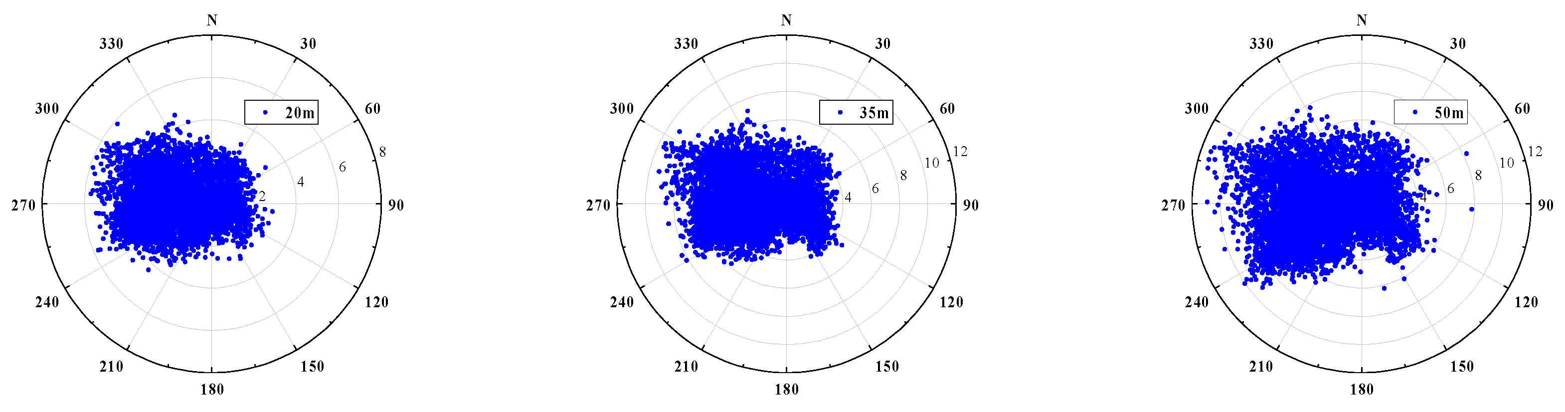
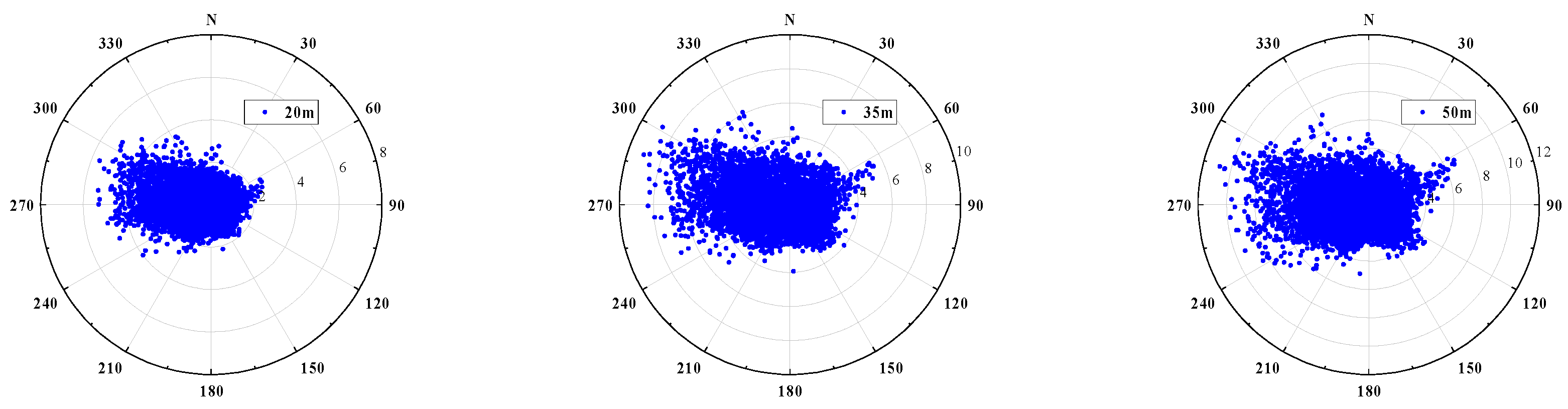
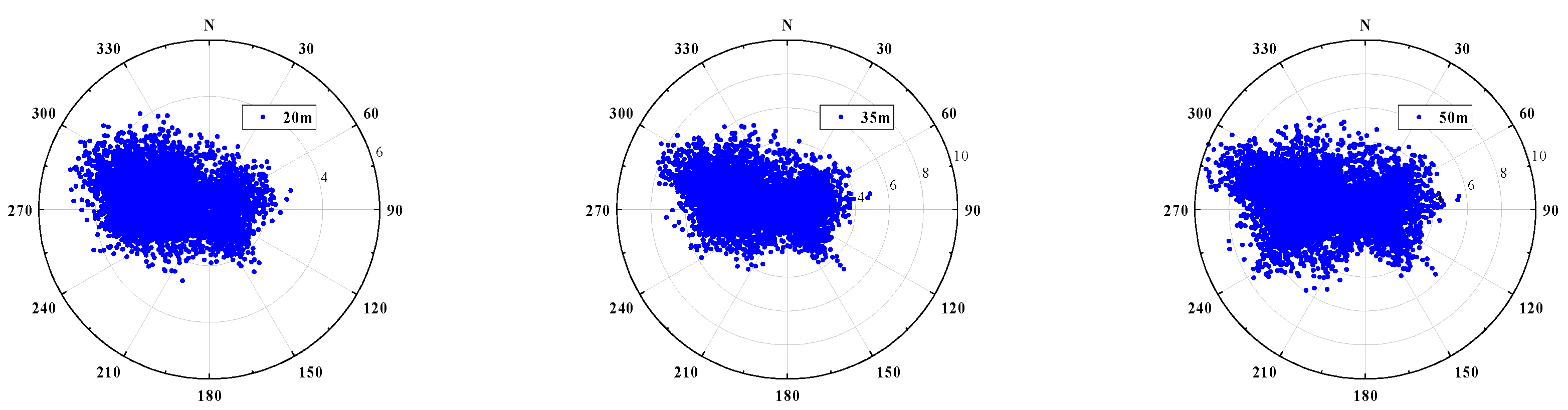
3.2. Mean Wind Directions

As wind-sensitive slender structures in forestry engineering sites have different wind-resistant performances in different wind directions, the mean wind direction plays an important role in the aerostatic stability of slender structures (e.g., wind turbines). Therefore, the mean wind direction of the flux tower at different heights and seasons was studied to reveal the effect of height and season on wind direction.

Figure 6, Figure 7, Figure 8 and Figure 9 show that when the mean wind speed threshold is set to 4 m/s, the variation of the mean wind direction ranges from 240° to 300° in spring, 240° to 300° and 60° to 150° in summer, and 270° to 300° in autumn and winter. The results show that the mean wind direction is significantly influenced by the seasons because the Maoer mountain region belongs to the monsoon climate zone and is mainly influenced by the northwest monsoon in autumn and winter due to the significant differences in land and sea thermal properties. Still, the temperature difference between summer and autumn/winter is large and the canopy is strongly disturbed. Cyclone activities are frequent, resulting in no obvious main wind direction for the mean wind direction in summer. Meanwhile, the figures show no significant variation in wind direction along the measured height, which means that the wind direction varies similarly at different heights. This also confirms that the seasonal influence on the mean wind direction is stronger than the variation with height.

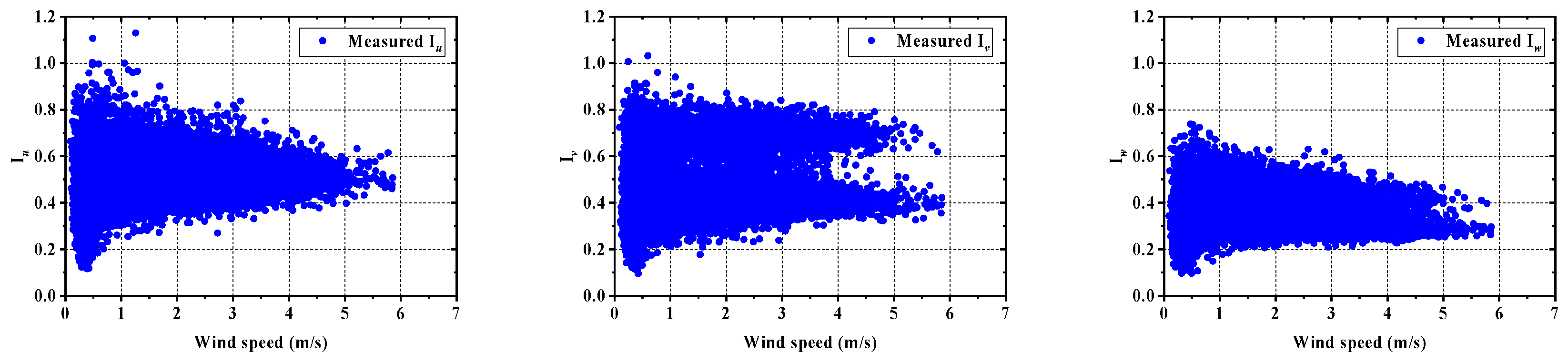
3.3. Turbulence Intensity

The airflow is affected by the surface roughness, which increases the fluctuating characteristics. Turbulence intensity is an important parameter indicator to characterize the strength of fluctuating winds, defined as the ratio of the standard deviation of the fluctuating wind component to the mean wind speed (10 min mean wind speed is used in this paper):

$$I_i=\frac{{\sigma }_i}{\overline{U}};\left(i=u,v,w\right)$$

(7)

where I_i is the turbulence intensity, σ_i is the standard deviation of the fluctuating wind components, and $\overline{U}$ is the mean wind speed.

Turbulence intensity is one of the most important wind field characteristics in the structural wind-resistant design [38,39,40], especially critical for the buffeting response of slender structures in forestry ecological regions and for the fatigue and ultimate loads of high-rise structures. For example, the turbulence intensity has an important effect on the vortex induced vibration and the aeroelastic stability due to the self-excited vibration. Since low wind velocity is responsible for vortex induced vibration and high wind velocity is major in aeroelastic stability, turbulence intensity should be investigated at low and high wind velocities. This paper conducted a comprehensive study of turbulence intensity in the forested region in different seasons, wind speed data were obtained from ultrasonic anemometers.

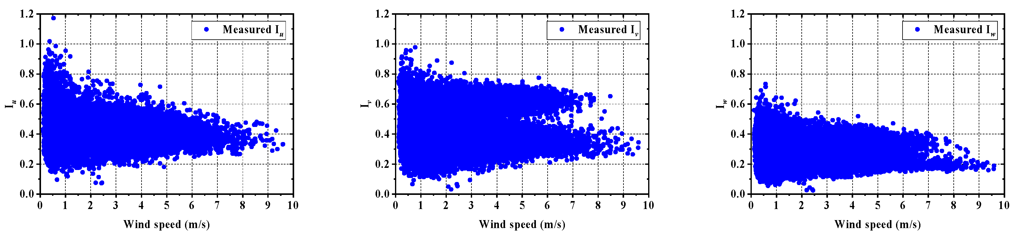
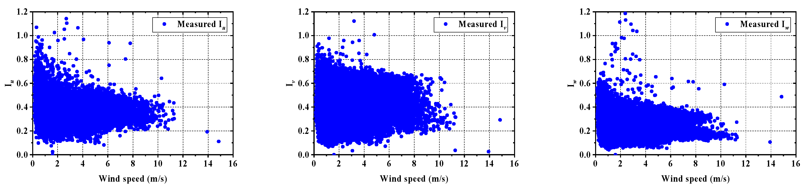
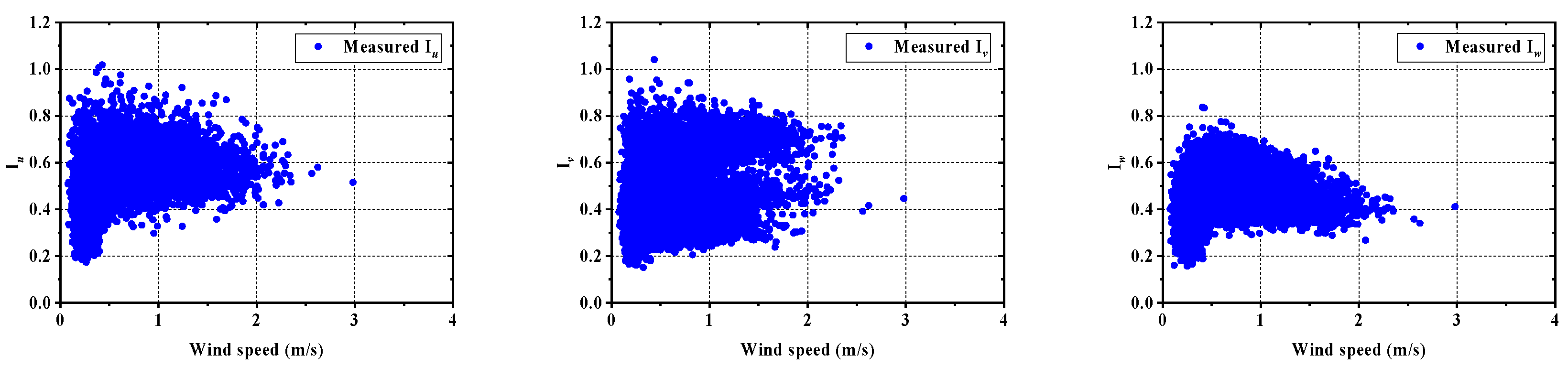
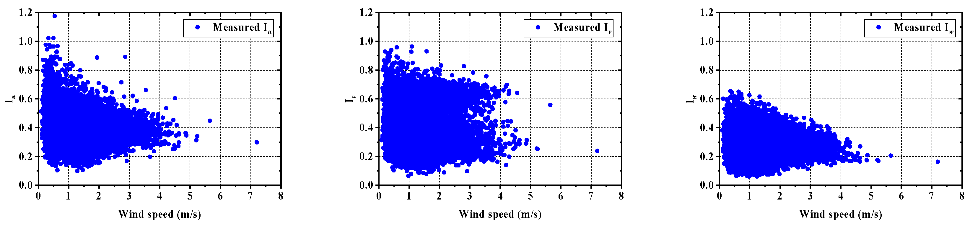
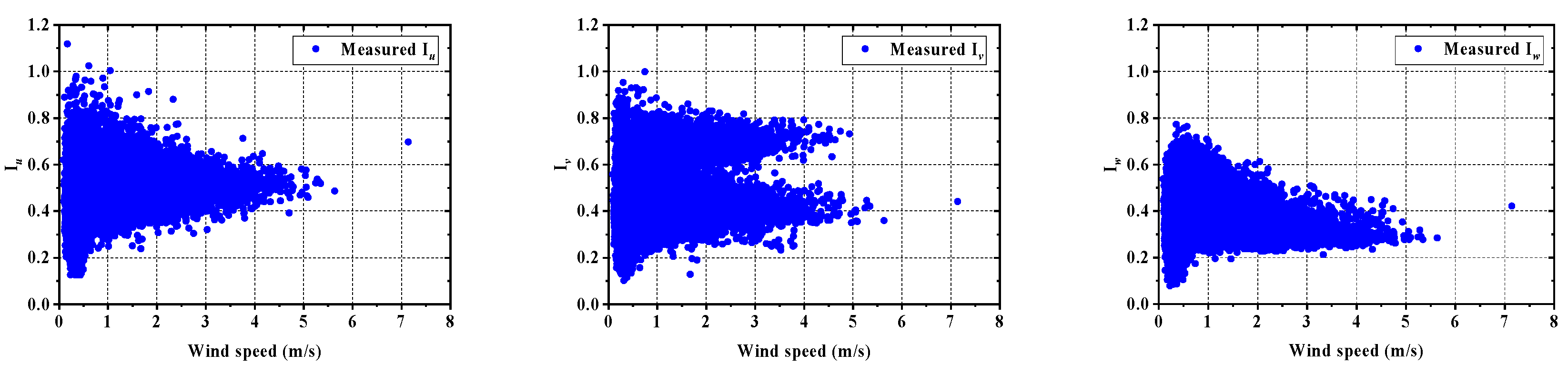
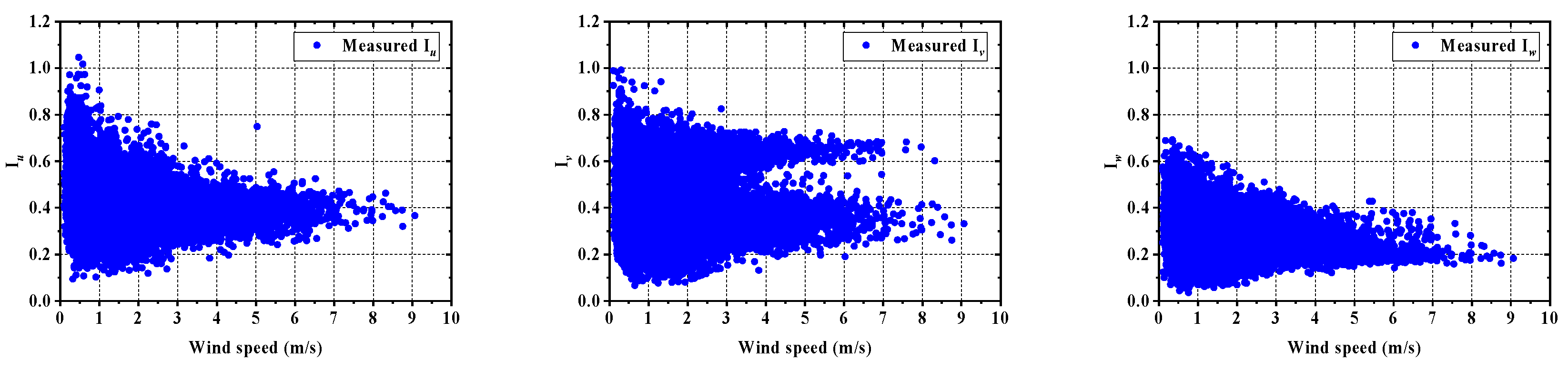
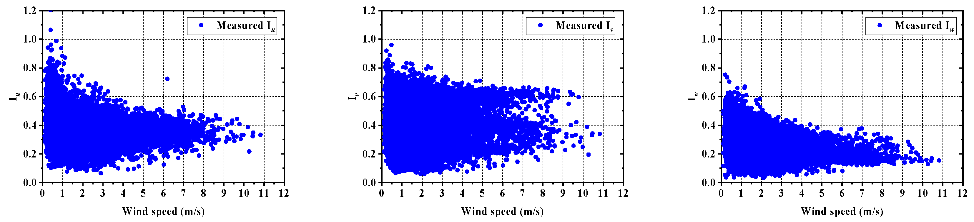
3.3.1. Variation with Wind Speed

According to Equation (7), the turbulence intensity decreases with increased wind speed. However, to further understand the variation of turbulence intensity with wind speed in complex terrain forested regions in different seasons, a mean wind speed threshold of 1 m/s was used to calculate the turbulence intensity, as shown in Figure 10, Figure 11, Figure 12, Figure 13, Figure 14, Figure 15, Figure 16, Figure 17, Figure 18, Figure 19, Figure 20 and Figure 21. These plots show that the turbulence intensity in the longitudinal, vertical, and 50 m height lateral directions decreases rapidly with increasing wind speed in the four seasons. However, the turbulence intensity in the 20 m and 35 m height lateral directions shows a new trend with increasing wind speed, which slowly decreases with increasing wind speed at low wind speeds. This trend is stronger in spring, when temperatures are unstable and windy than in autumn and winter, while it becomes dominant in summer. This also states that in spring, autumn, and winter I_v converges to two values, while in summer I_v has no significant convergence values.

In addition, it can be seen from Figure 10, Figure 11, Figure 12, Figure 13, Figure 14, Figure 15, Figure 16, Figure 17, Figure 18, Figure 19, Figure 20 and Figure 21 that with the increase in wind speed, the three turbulence intensity components I_u, I_v, and I_w at each height in each season tend to have different values, for example, the three components at 50 m height in winter tend to 0.33, 0.31, and 0.14, respectively, and the ratio should be close to 1:0.93:0.42, which is very different from the Chinese specification (JTG/T 3360-01. 2018) [23] which recommends a ratio of 1:0.88:0.50. Therefore, it is not appropriate to apply the turbulence components ratios proposed in the specifications and standards to the wind-resistant design of wind-sensitive structures located at forested engineering sites under high wind speed conditions. Moreover, as the wind speed increases, the lateral turbulence intensity converges to two values in spring, autumn, and winter. The convergence value is not obvious in summer, making the three turbulence intensity component ratios more complex and diverse and statistically inconsistent with the recommended values. Therefore, the wind-resistant design of adaptive engineering measures such as aerial ropeways and transmission towers located in forested regions should consider the actual turbulence intensity in different seasons.

3.3.2. Variation with Height

For wind-sensitive structures in forested regions, it is difficult to obtain turbulence intensities at all ideal locations (e.g., on top of aerial ropeways and wind turbine towers) through in field measurements. Only the turbulence intensity near the measurement point at a specific height can be obtained in most cases. Moreover, from Equation (7), the mean and standard deviation of turbulence intensity decreases with the increase in height. To further understand how the turbulence intensity varies with height in different seasons and how it affects the structure, data from flux towers at 20 m, 35 m, and 50 m were analyzed.

Some specifications [21,22,23] suggest that the longitudinal turbulence intensity can be expressed as a power law [41]. The empirical formula is as follows:

$$I_u\left(z\right)=c{\left(\frac{10}{z}\right)}^d$$

(8)

The empirical formula in Chinese code has been specifically defined as:

$$I_u\left(z\right)=I_{10}{\left(\frac{10}{z}\right)}^{\alpha }$$

(9)

where α is the terrain roughness coefficient and I₁₀ is the nominal turbulence intensity at a height of 10 m (determined from four typical standard wind terrains) [41].

For convenience, the above empirical equation was used to analyze turbulence intensity in the forested region. The parameters c and d (I₁₀ and α) are obtained by fitting the least-squares method to the turbulence intensity using the empirical formula. The mean turbulence intensity and the mean and standard deviation of the c and d parameters were calculated separately during data processing to study the turbulence intensity variation with height in the forested region. The fitting results are shown in Figure 22, Figure 23, Figure 24 and Figure 25, and the PDF distributions of the fitted parameters c and d are shown in Figure 26, Figure 27, Figure 28, Figure 29, Figure 30, Figure 31, Figure 32, Figure 33, Figure 34, Figure 35, Figure 36 and Figure 37.

As can be seen from Figure 22, Figure 23, Figure 24 and Figure 25, the turbulence intensity profiles for each season agree well with the above empirical equations. It can be concluded that it is reasonable to apply the power-law formula to describe the variation of turbulence intensity with height in forested regions in different seasons. Figure 22, Figure 23, Figure 24 and Figure 25 show that the fitted parameters c conform to the law c_u > c_v > c_w in spring, autumn and winter (longitudinal > lateral > vertical), but this law does not apply in summer when the temperature is high and the canopy is dense. For the fitted parameter d, the d_w > d_u > d_v rule is satisfied in all seasons. However, the fitted parameters c and d (I₁₀ and α) of the three turbulence intensity components vary greatly from season to season, with the largest fitted parameters in summer. This may be caused by the significant difference in turbulent winds at 20 m and 35 m height caused by high temperature and dense canopy in summer. This proves that the surface roughness is seriously affected by the seasons. Additionally, the fitted parameters for each season c and d (I₁₀ and α) differed significantly from those recommended by specifications or standards. Moreover, the three turbulence intensity components not only differ greatly in magnitude, but they also have different correlation coefficients with height. It can also be seen from Figure 22, Figure 23, Figure 24 and Figure 25 that the standard deviation of turbulence intensity is large in all seasons and varies less with height. This demonstrates that the power law function can be used to predict the turbulence intensity in forested regions, but it needs to be based on the field measurements in each season.

As shown in Figure 26, Figure 27, Figure 28, Figure 29, Figure 30, Figure 31, Figure 32, Figure 33, Figure 34, Figure 35, Figure 36 and Figure 37, the PDF distribution of the parameter c for each season obeys well the lognormal distribution. The parameter c is I₁₀ of Chinese specification. The PDF distribution of parameter d conforms to the Gaussian distribution (normal distribution), that is, the PDF of the terrain roughness coefficient obeys a Gaussian distribution in all seasons in the forested region. The shape of the PDF obtained in this paper is consistent with the shape given in the reference [42], while the literature states that the parameter d (terrain roughness coefficient α) varies with wind speed, and at high wind speeds, the terrain roughness coefficient α may be more reasonable. Therefore, the parameters variation with wind speed is shown in Figure 38, Figure 39, Figure 40 and Figure 41. The results show that the parameter d converges to one value in the longitudinal and vertical directions for each season as the wind speed increases, while the lateral wind law differs from it, with the parameter d converging to one value in spring, autumn, and winter, and converging to one range in summer, influenced by the dense vegetation in the forested region. Meanwhile, the convergence values of the parameter d in the three directions in each season do not differ much from those given in Figure 22, Figure 23, Figure 24 and Figure 25, and the convergence range remains centered on the parameter d given in Figure 23 even for the lateral wind direction in summer. Therefore, for convenience, the parameters c and d of the turbulence intensity profile for each season can be chosen according to the power-law function. It is also pointed out that in forested regions, applying actual field measurement data to calculate seasonally fitted parameters, rather than based on specifications or standards, is more suitable for forest engineering applications.

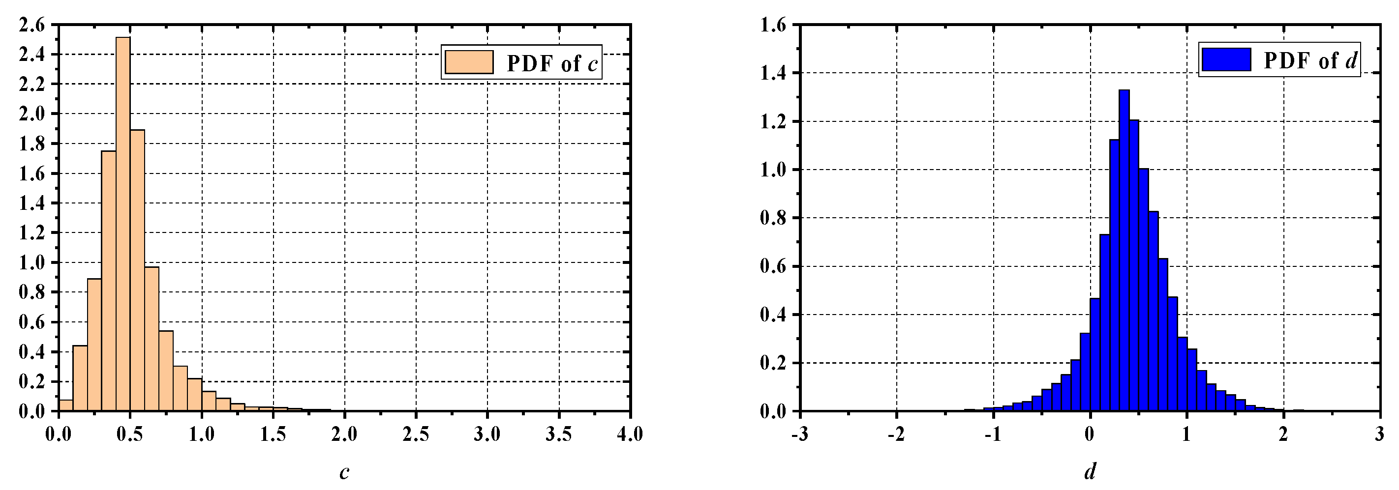
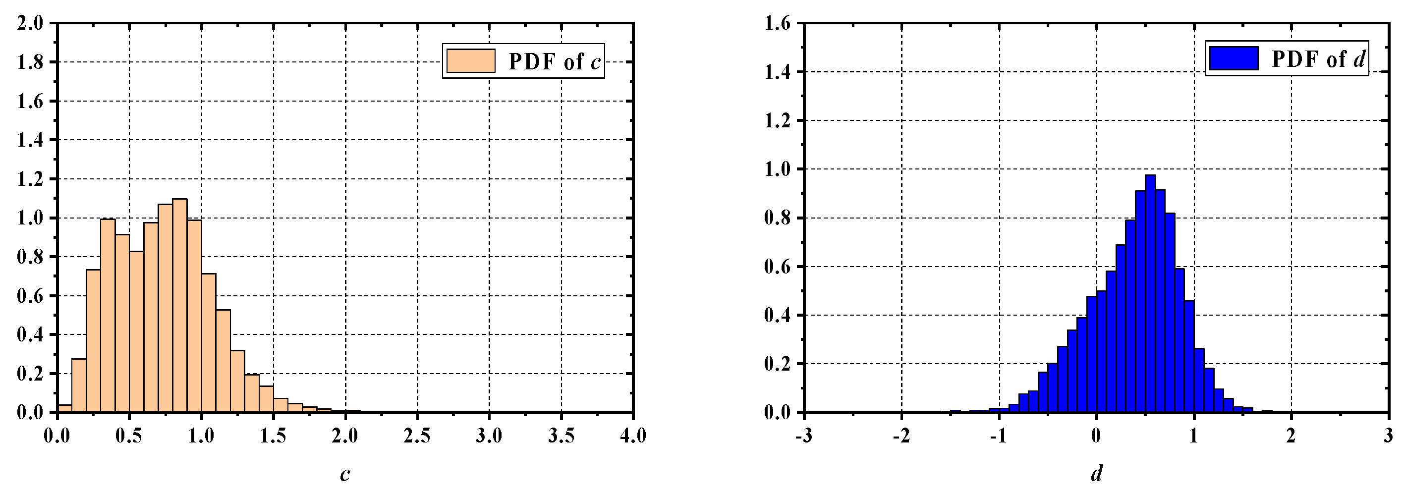
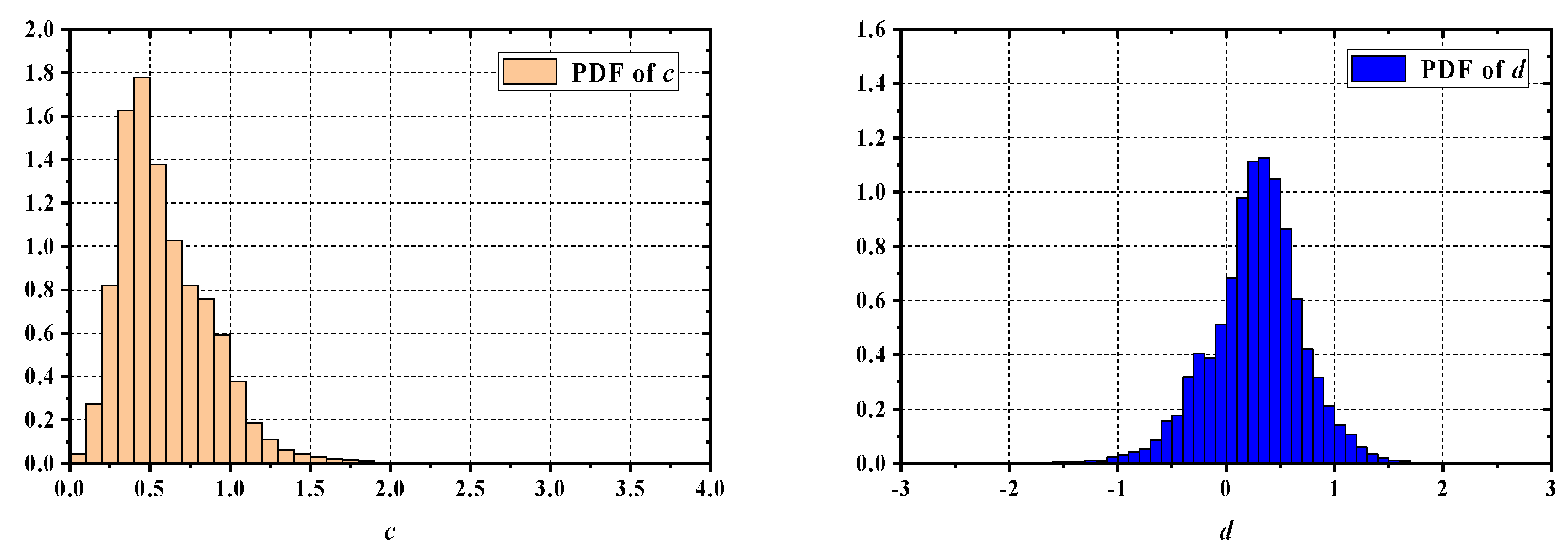
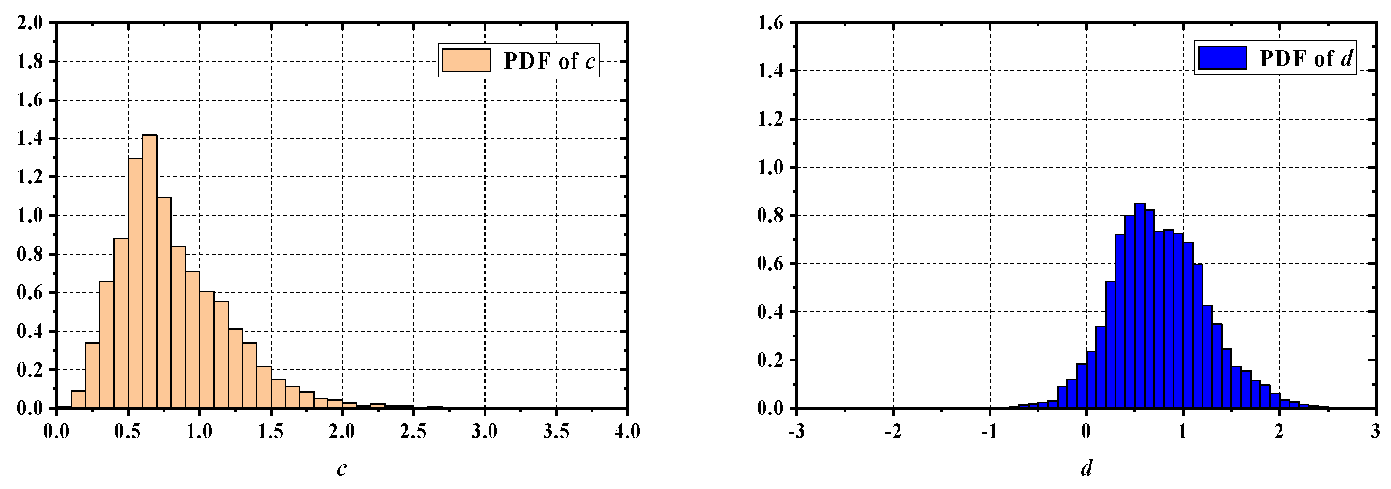
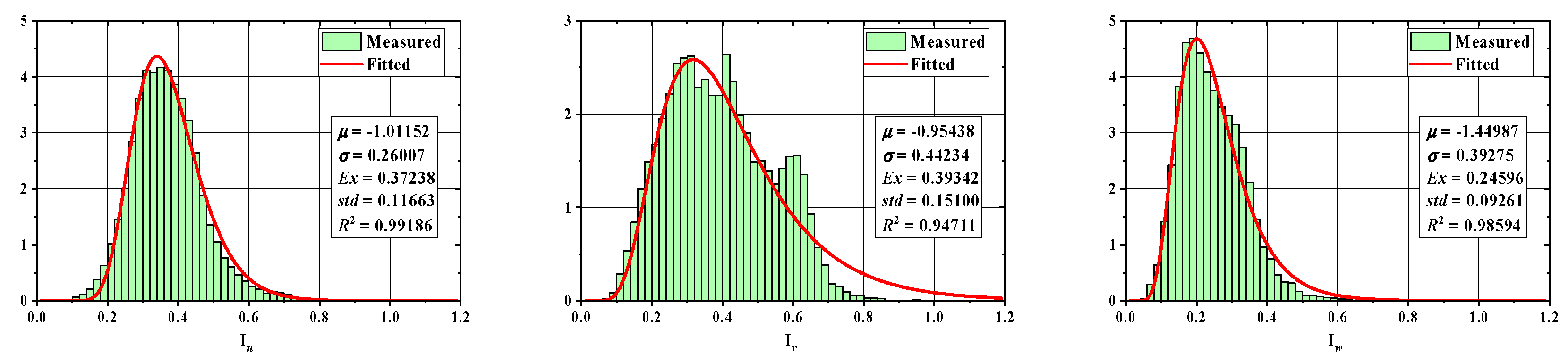
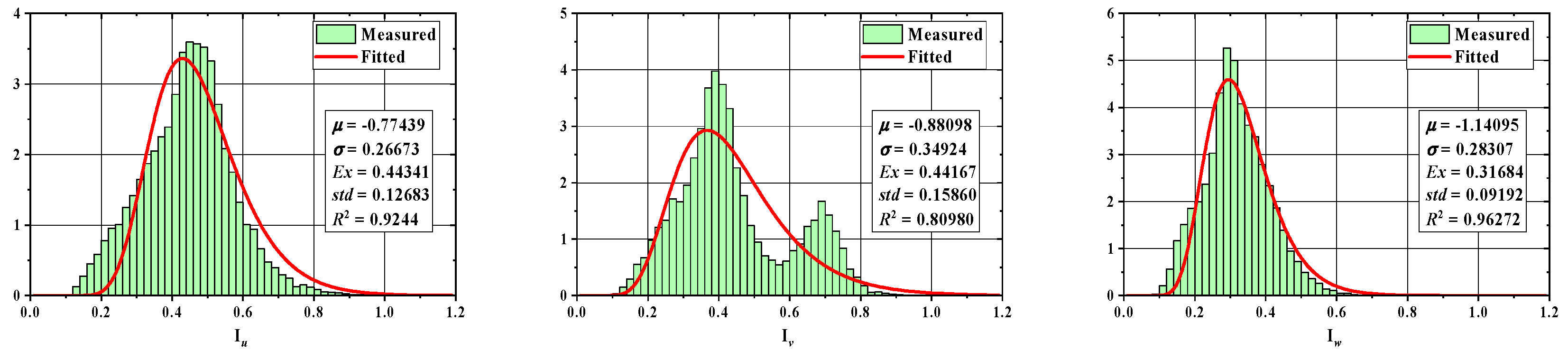
3.3.3. PDF Distribution

A large number of current academic studies and specifications show that the PDF distribution of turbulence intensity coincides well with the log-normal distribution, which is expressed as follows:

$$f\left(x\right)=\frac{1}{x\sigma \sqrt{2\pi }}{e}^{-\frac{{\left(\ln x-\mu \right)}^2}{2{\sigma }^2}};x>0$$

(10)

where μ and σ denote the mean and standard deviation of the natural logarithm of the variable x.

However, the turbulence in complex terrain forested regions is complicated and significantly influenced by the season. It is difficult to know whether the above expressions apply to this terrain type. Therefore, to study the distribution of turbulence intensity probability density function in complex terrain forest regions in detail, the wind speed data collected by ultrasonic anemometer (20 m, 35 m, and 50 m height from the ground, respectively) were studied exhaustively.

The PDF distribution of turbulence intensity at 20 m, 35 m, and 50 m heights for each season are shown in Figure 42, Figure 43, Figure 44, Figure 45, Figure 46, Figure 47, Figure 48, Figure 49, Figure 50, Figure 51, Figure 52 and Figure 53. The results show that the PDF distribution of the turbulence intensity in the longitudinal and vertical directions in different seasons can be expressed by lognormal distribution with appropriate parameter conditions, while the turbulence intensity in the lateral wind direction at 20 m and 35 m height is seriously affected by the disturbance of tree canopy and branches, the PDF distribution shows a bimodal trend, and the lognormal distribution cannot well represent the turbulence intensity in the lateral wind direction in each season. It indicates that the high turbulence intensity occupies a significant role in the lateral wind direction and low height, influenced by the complexity of the wind field in the forest region. Meanwhile, the bimodal trend of PDF distribution also confirms two trends of lateral turbulence intensity with wind speed. Especially, dense vegetation in summer causes the turbulence intensity in the lateral direction to be greater than the other three seasons and the PDF distribution expressed by the lognormal distribution fits better than the other three seasons. A 50 m height is less affected by the near-ground roughness, and the lateral PDF can be expressed by the lognormal distribution (R² > 0.9). Meanwhile, the fitted parameters μ and σ, as well as the standard deviations and mathematical expectations derived from μ and σ according to the lognormal distribution property are also shown in Figure 54, Figure 55, Figure 56 and Figure 57. It can be seen that, in general, the fitted parameter μ decreases faster with increasing height in spring, summer, and winter, the expectation and standard deviation decrease very slowly with increasing height, and the parameter σ increases with increasing height, while there is no obvious law for the fitted parameter, expectation, and standard deviation in autumn. This also demonstrates the importance of seasonal influences on the wind-resistant design of engineering sites in forested regions with complex terrain.

The ratios of each component of turbulence intensity are shown in

Table 2. Ratio amongst components of turbulence intensity in seasons.

Height	Season	Iu:Iv:Iw
20 m	Spring	1:0.998:0.75
	Summer	1:0.927:0.909
	Autumn	1:0.986:0.833
	Winter	1:1.038:0.748
35 m	Spring	1:1.07:0.6 71
	Summer	1:1.043:0.686
	Autumn	1:1.033:0.67
	Winter	1:1.115:0.644
50 m	Spring	1:1.099:0.674
	Summer	1:1.035:0.693
	Autumn	1:1.056:0.671
	Winter	1:1.165:0.639

. The results show that the ratio has no definite value with different heights and seasonal variations. It can be seen from the table that the ratio of vertical turbulence intensity to longitudinal turbulence intensity is the largest in summer and the smallest in winter. The ratio of lateral turbulence intensity to longitudinal turbulence intensity is the largest in winter and the smallest in summer. Meanwhile, the ratio of lateral turbulence intensity to longitudinal turbulence intensity increases with increasing height and the ratio of vertical turbulence intensity to longitudinal turbulence intensity decreases with increasing height in all seasons. The results showed that the greater the vertical to longitudinal ratio, the hotter the climate and the denser the canopy, and the greater the lateral to longitudinal ratio, the colder the climate and the sparser the canopy. This may be due to the fact that lateral and vertical turbulent winds are affected differently by the seasons. However, it is known that some specifications and standards propose a ratio between the various components of turbulence intensity. For example, the ratio suggested in the Chinese specification is 1:0.88:0.50. As can be seen from Table 2, the proposed ratios differ significantly from those obtained from the field measurements in each season. It follows that it is not appropriate to apply specifications and standards directly to forested regions. Therefore, it is necessary to obtain the turbulence intensity in each season in the forested region by field measurements or other methods.

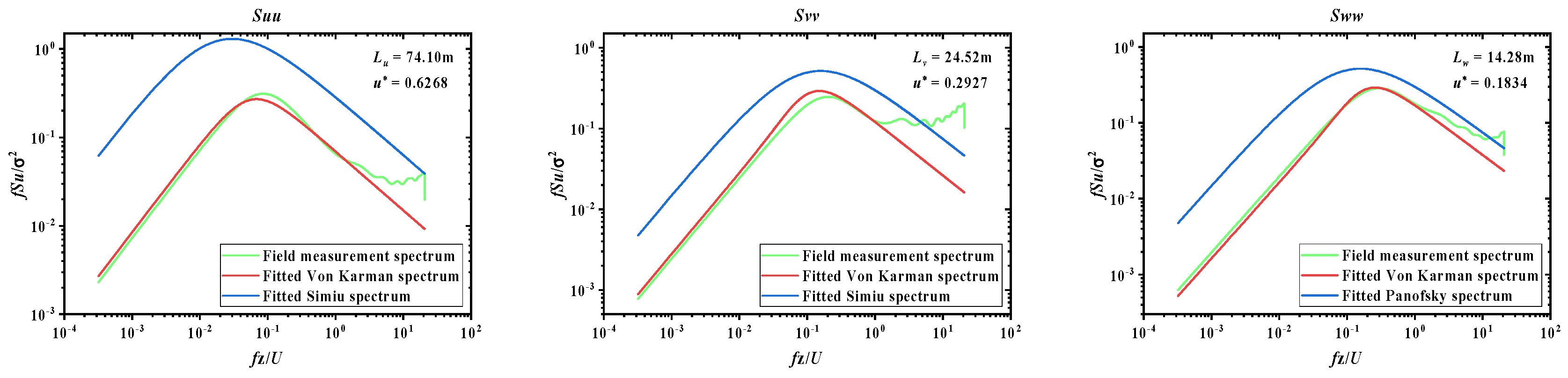
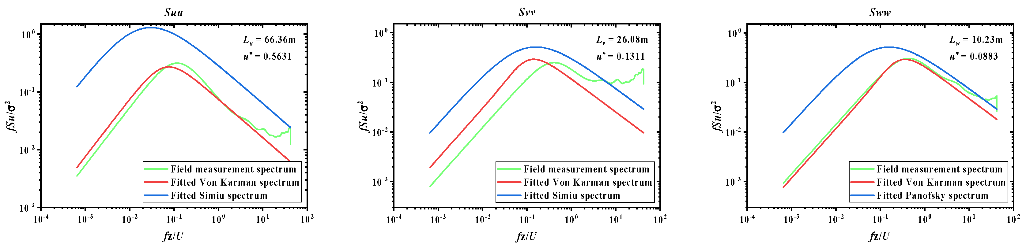
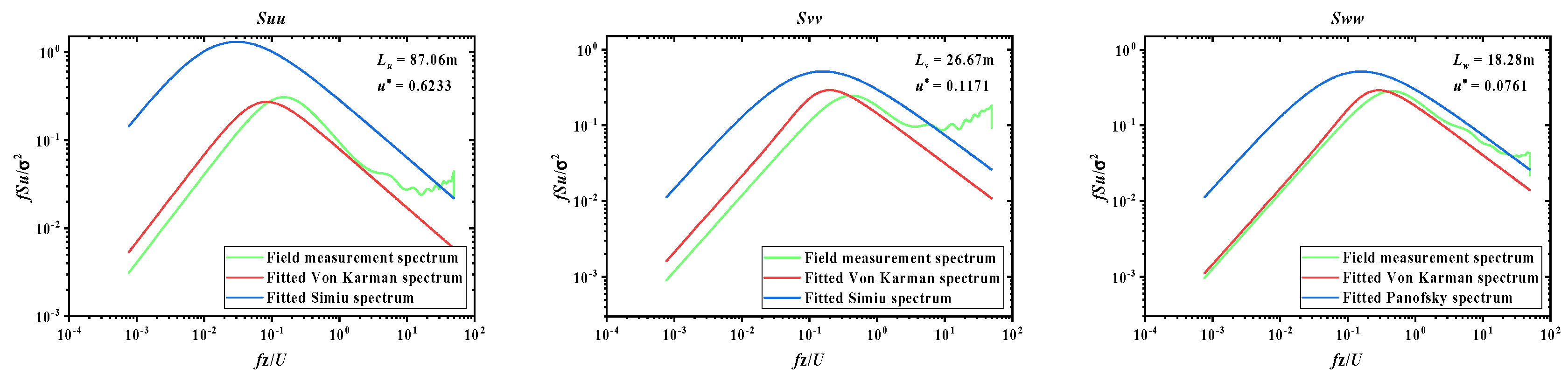
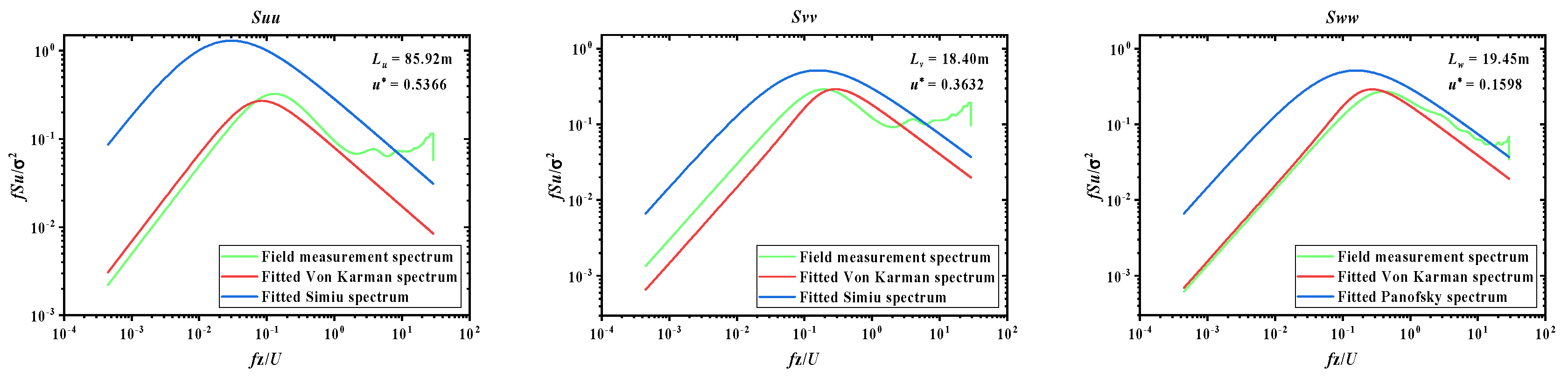
3.4. Turbulent Spectrum

The turbulent wind spectrum is another important parameter to describe the fluctuating wind characteristics, which can characterize the distribution profile of turbulent energy in each frequency domain. To obtain the functions of turbulent wind speed spectrum expressions, many scholars have conducted a large number of field measurements and wind tunnel experimental studies and proposed wind spectrum models such as the Von Kármán spectrum, Davenport spectrum, Simiu spectrum, Kaimal spectrum, and Panofsky spectrum [43,44,45,46,47,48]. For example, Chinese codes employ the Simiu spectrum [43] to depict the longitudinal and lateral wind spectra and the Panofsky spectrum [45] to the vertical [48]. The empirical formulas are as follows:

For the longitudinal wind spectrum, the Simiu spectrum is

$$\frac{f\cdot S_u\left(f,z\right)}{u_{\ast }^2}=\frac{200f_z}{{\left(1+50f_z\right)}^{5/3}}$$

(11)

For the lateral wind spectrum, the following modified spectrum is

$$\frac{f\cdot S_v\left(f,z\right)}{u_{\ast }^2}=\frac{15f_z}{{\left(1+9.5f_z\right)}^{5/3}}$$

(12)

For the vertical wind spectrum, the Panofsky spectrum is

$$\frac{f\cdot S_w\left(f,z\right)}{u_{\ast }^2}=\frac{6f_z}{{\left(1+4f_z\right)}^2}$$

(13)

where f is the frequency in Hz; S_u,v,w(f, z) is the turbulent wind spectrum at ground height z; u_* is the friction wind speed; and fz is the non-dimensional reduced frequency, which is expressed as

$$f_z=\frac{f\cdot z}{U\left(z\right)}$$

(14)

where U (z) is the mean wind speed at height z above ground.

Moreover, according to a large number of field measurement studies, the Von Kármán spectrum is considered one of the most suitable wind spectra for representing fluctuating wind speeds at high wind speeds, which is expressed as:

$$\frac{f\cdot S_u\left(f,z\right)}{{\sigma }_u^2}=\frac{\frac{4L_u\cdot f}{U}}{{\left[1+70.8{\left(\frac{L_u\cdot f}{U}\right)}^2\right]}^{5/6}}$$

(15)

$$\frac{f\cdot S_{v,w}\left(f,z\right)}{{\sigma }_{v,w}^2}=\frac{\frac{4L_{v,w}\cdot f}{U}\left[1+188.4{\left(\frac{2L_{v,w}\cdot f}{U}\right)}^2\right]}{{\left[1+70.8{\left(\frac{2L_{v,w}\cdot f}{U}\right)}^2\right]}^{11/6}}$$

(16)

where L_u,v,w are the longitudinal, lateral, and vertical turbulent integral length scales, respectively; σ_u,v,w are the standard deviations of the longitudinal, lateral, and vertical turbulent components, respectively; and U is the mean wind speed.

Considering the complex wind environment in various seasons in forested regions, the turbulent wind spectrum may not be characterized by a single Simiu spectrum, Panofsky spectrum, or Von Kármán spectrum. Therefore, since fluctuating winds play an important role in the design of structural wind resistance, this paper investigates the field measurements of ultrasonic anemometer records to obtain turbulent wind spectra.

To better study the variation law of turbulent power spectrum, the MATLAB pyulear function can be applied for power spectral density estimation. Liao [36] processed raw wind data by applying the pyulear function of order 15 and the pwelch function. It can be concluded that the wind spectrum obtained with the pyulear function is smoother than that obtained with the pwelch function, and it is very convenient to obtain the peak frequency. Therefore, the pyulear function of order 15 was chosen to analyze the measured data for the four seasons.

To investigate the applicability of the above spectra, the fitted Simiu, Panofsky, and Von Kármán spectra are also illustrated with the corresponding measured spectra. To unify coordinates, the height is used to normalize the frequency. Due to the forested region’s high complexity, the forest canopy has a blocking effect significantly impacts the near-ground turbulent spectrum. This effect may weaken with increasing height. Field-measured spectrums at different heights (20 m, 35 m, and 50 m) were calculated from the raw wind speed data in different seasons to further understand the turbulent spectrum variation with height.

Figure 58, Figure 59, Figure 60, Figure 61, Figure 62, Figure 63, Figure 64, Figure 65, Figure 66, Figure 67, Figure 68 and Figure 69 compare the field measurement spectra with the fitted spectra at 20 m, 35 m, and 50 m heights in different seasons. As can be seen from the figures, the Von Kármán spectral model can more accurately reflect the longitudinal and vertical field measurement spectra at three heights in different seasons. For the lateral field measurement spectra, only the winter, spring 35 m, and summer 20 m field measurement spectra are more closely matched to the Von Kármán spectrum. Because the winter is a leafless period in the northeastern forested region, the near-ground roughness is small compared with other seasons, and the lateral wind direction is less disturbed leading to a reduction in fluctuating wind amplitude, but as the spectrum moves toward the high-frequency domain, the lateral field measurement spectrum differs more from the Von Kármán spectrum. In contrast, the Simiu and Panofsky spectral models provided by the Chinese specification differ too much from the field measurement spectra and overestimate the field measurement spectra. It can also be seen that the shapes of the longitudinal, lateral, and vertical spectra are essentially constant at different heights, and that the Von Kármán spectrum increasingly fits the field measurement spectrum as the height increases, but the opposite trend is observed in the high-frequency domain after passing through the high-energy region (peak). Figure 58, Figure 59, Figure 60, Figure 61, Figure 62, Figure 63, Figure 64, Figure 65, Figure 66, Figure 67, Figure 68 and Figure 69 supplement the relevant parameters’ values. The turbulence integral length scale in the three directions increases with height, where it is severely disturbed by the dense forest canopy (due to compression, cutting, and other effects), and the turbulence integral length scale at 20 m height in summer is about 0.43 times higher than that in other seasons. Additionally, the friction velocity decreases with increasing height, but the friction velocity in summer, which is severely affected by surface roughness, is not large, probably because the observed wind speed is too small. Therefore, it is not appropriate to use a spectral model with definite parameters to calculate the vibration response of an engineered structure located in a forested region. The turbulent spectra are different in different seasons. However, they are at the same height point, which is interesting in calculating the vibration response of wind-sensitive structures in forested regions. In general, the wind spectrum model should be carefully selected concerning the field measurements.

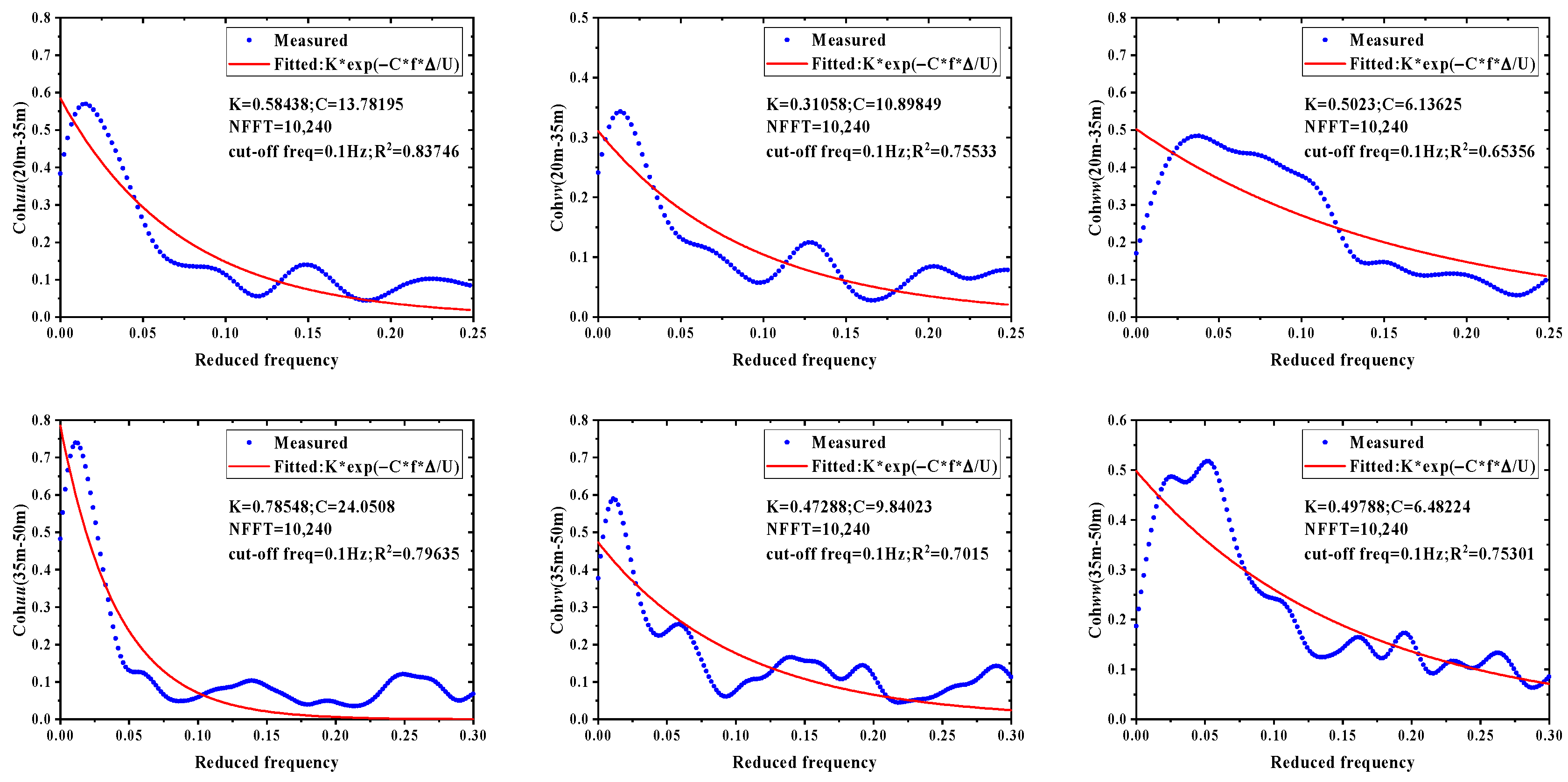
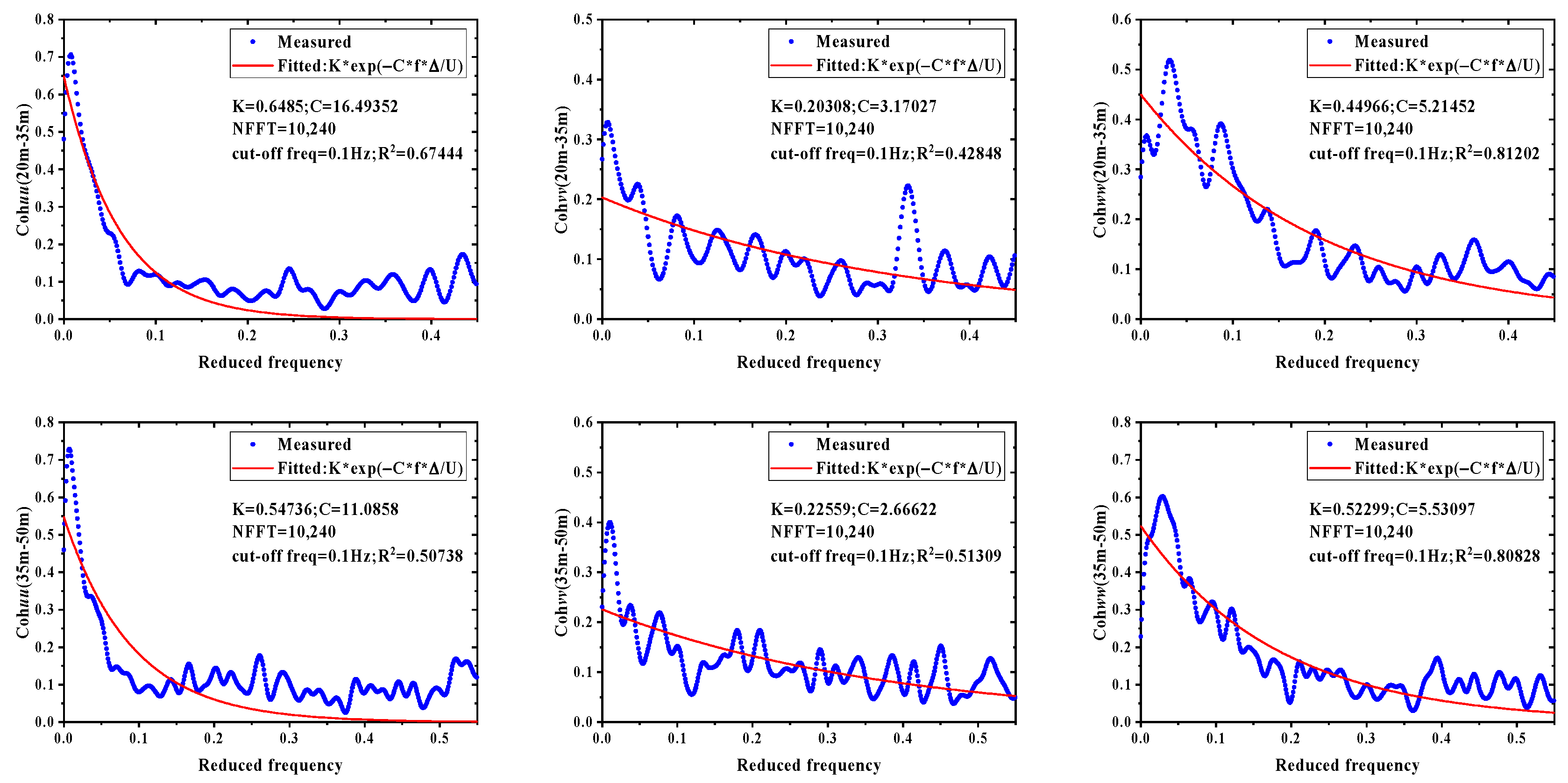
3.5. Vertical Spatial Coherence

The coherence function in the frequency domain can describe the statistical dependence of the fluctuating wind speed at any two points. It is usually defined as the ratio of the cross-spectral density to the auto-spectral density of the fluctuating wind speed at any two points [45,49]. The definition is as follows:

$$C_{xy}\left(f\right)=\frac{{\left|P_{xy}\left(f\right)\right|}^2}{P_{xx}\left(f\right)P_{yy}\left(f\right)}$$

(17)

where C_xy denotes the coherence estimates of the fluctuating wind speeds x (t) and y (t) using Welch’s averaged periodogram method; P_xy denotes the cross-spectral density of the fluctuating wind speeds x (t) and y (t); P_xx and P_yy denote the auto-spectral density of the fluctuating wind speeds x (t) and y (t), respectively.

In previous research, many empirical formulas for spatial coherence have been proposed. Davenport [44] suggested an exponential format of coherence formulas to represent horizontal and vertical coherence:

$$C_{xy}\left(f\right)=\frac{{\left|P_{xy}\left(f\right)\right|}^2}{P_{xx}\left(f\right)P_{yy}\left(f\right)}$$

(18)

where C is the decay coefficient; Δ is the separation distance between the two points. However, according to more field measurement studies, the coherence is not equal to 1 when the frequency is close to 0. Later, Mann [50] improved the above equation to better fit the measured data. The improved formula is:

$$Coh\left(f\right)=\sqrt{\left(1-B\cdot \frac{\Delta }{z}\right)}\exp \left(-C\cdot \frac{f\cdot \Delta }{U}\right)$$

(19)

In addition, for concision, a modified coherence formula is derived from the above equation as [47]:

$$Coh\left(f\right)=K\cdot \exp \left(-C\cdot \frac{f\cdot \Delta }{U}\right)$$

(20)

where B and K are parameters to be fitted; z is the height above ground.

In general, the above coherence equation may not be applicable due to the complex wind environment in forested regions. Therefore, to verify whether the above coherence Equation (20) can be used to represent the coherence of the forested region, the vertical coherence functions for measured data are calculated using MATLAB’s mscohere function with NFFT = 10,240 in this paper, a comparison between measured data and the above coherence model was performed. In addition, the coherence functions for measured data are also studied to further reveal the variation with height. Coherence analysis was performed on the field measurement data of 20 m, 35 m and 35 m, 50 m in the four seasons.

As seen from Figure 70, Figure 71, Figure 72 and Figure 73, Formula (20) can better represent the vertical coherence of the field measurements in the four seasons. In addition, when the frequency converges to zero, the measured coherence of the three components of the four seasons in the forested region does not converge 1. This indicates that Formula (18) is not applicable in complex terrain forest regions. Formulas (19) and (20) are appropriate, but Formula (20) is more concise. For different turbulence components in the same season and at the same two points, the fitted values K and C are not identical. For the same vertical distance, the fitted values K and C also differ. The fitted values K and C were more different in different seasons. The measured coherence indicates that the lateral fitted values K and C are the smallest, and lateral coherence drops slower than longitudinal and vertical coherence. This may be caused by the strong disturbances of lateral turbulent wind arising from rugged terrain and vegetation. This conclusion also has been proved in Section 3.3. Even when the distance between the two points is constant, the coherence of the components is not the same for both ascending and descending measured heights, which indicates that turbulent vortices are not consistent at different heights within the forested region. This conclusion also has been proved in the measured spectra.

To investigate the variation of the fitted values K and C with season and height, the results are shown in Figure 74 and Figure 75. For the longitudinal direction, the fitted parameters K and C increased with increasing height in spring and summer and decreased with increasing height in autumn and winter. For the lateral direction, the fitted parameter K increases with height, the fitted parameter C increases with height in spring and winter, and the opposite in summer and autumn. For vertical direction, the four seasonal-fitted parameters K and C increase with increasing height. This indicates that the fitted parameters K and C do not have a defined seasonal variation law; therefore, in engineering applications, we should not rely on the coherence function of the defined parameters, but on the seasonally fitted parameters calculated based on the field measurement data.

4. Concluding Remarks

Due to the wind field’s complexity, significant seasonal effects in forested regions and the lack of relevant studies, this paper presents comprehensive research on the wind field in forested regions using the on-site field measurement data. A comprehensive study of the mean and fluctuating wind characteristics was conducted using statistical methods. The results were compared between seasons and with the specifications and standards of many countries. The major conclusions of this study can be summarized as follows:

(1)

Due to the seasonal variation in the near-ground atmospheric boundary layer in the forested region, the mean wind speed profile exhibits different gradients in different seasons, while the mean wind direction also shows seasonal differences. Although the power-law model can capture the basic shape of mean wind speed profiles in forested regions in different seasons, the definite parameters in the standard cannot fully reflect the vertical distribution of wind speed, while the seasonally fitted parameters have higher applicability for better reproduction of mean wind profiles in forested regions where the roughness varies with season. The mean wind direction ranges from 270° to 300° in autumn and winter, 240° to 300° in spring, but 240° to 300° and 60° to 150° in summer, which indicates that the mean wind direction changes in summer due to temperature and pressure differences and canopy disturbances. It is also pointed out that the influence of season should be given priority for the mean wind direction.

(2)

The power-law function can predict the turbulence intensity profile in different seasons in the forested region. However, the fitted parameters differed significantly from season to season, while each turbulence intensity component converged at different values in different seasons at high wind speed conditions. This demonstrates the significant seasonal effects on the power-law function of turbulence intensity in forested regions. Meanwhile, the ratios of the three turbulence intensity components are significantly affected by the seasons, with low ratios in the vertical and longitudinal directions for the cold and canopy-sparse autumn and winter, and low ratios in the lateral and longitudinal directions for the hot and canopy-rich summer. This indicates that the ratio of turbulence intensity components proposed by specifications and standards is not adapted to the forest engineering sites. In addition, three directions’ PDF distributions have different μ and σ parameters in different seasons at different heights, while the log-normal distribution can better characterize the longitudinal and vertical turbulence intensity in each season and the PDF distribution at the lateral 50 m height. However, canopy and branch disturbances affect the lateral turbulence intensity at 20 m and 35 m height, and the log-normal distribution does not characterize the lateral PDF distribution well in each season with a bimodal trend.

(3)

The Simiu and Panofsky spectral model no longer applies to turbulent fields in the forested region in all seasons. However, the Von Kármán spectrum still has important applicability for such topographic sites. The longitudinal, lateral, and vertical component spectral models remained constant with increasing height each season but were not similar between the components. The turbulent spectrum differs in various seasons, although they are points at the same height. In addition, the turbulence integration length scale in all three directions increases with height. This paper shows that the turbulent flow spectrum with definite parameters no longer applies in the forested region.

(4)

The modified empirical coherence formula can better reflect the vertical spatial coherence in the four seasons in the forested region with appropriate parameters. In the forested region, the lateral coherence in seasons is weaker than the other two coherences, which corresponds to the PDF distribution of the turbulence intensity. Meanwhile, the fitted parameters K and C do not have consistent seasonal regularity in different directions. So, the seasonally fitted parameters fitted by field measurement data are essential for their vertical spatial coherence in engineering applications.

References

1. Giannaros, T.M.; Melas, D.; Ziomas, I. Performance evaluation of the Weather Research and Forecasting (WRF) model for assessing wind resource in Greece. Renew. Energy 2017, 102, 190–198. [Google Scholar] [CrossRef]
2. Hsiao, C.Y.L.; Sheng, N.; Fu, S.Z.; Wei, X.Y. Evaluation of contagious effects of China’s wind power industrial policies. Energy 2022, 238, 121760. [Google Scholar] [CrossRef]
3. Pena, A.; Floors, R.; Sathe, A.; Gryning, S.E.; Wagner, R.; Courtney, M.S.; Larsen, X.G.; Hahmann, A.N.; Hasager, C.B. Ten Years of Boundary-Layer and Wind-Power Meteorology at Hovsore, Denmark. Bound. -Layer Meteorol. 2016, 158, 1–26. [Google Scholar] [CrossRef] [Green Version]
4. da Silva, A.F.G.; de Andrade, C.R.; Zaparoli, E.L. Wind power generation prediction in a complex site by comparing different numerical tools. J. Wind Eng. Ind. Aerodyn. 2021, 216, 104728. [Google Scholar] [CrossRef]
5. Ying, C.; Wenyi, F.; Yibo, W. Study on Seasonal Dynamics of Leaf Area Index in Maoer Mountain. For. Eng. 2016, 32, 1–6. [Google Scholar] [CrossRef]
6. Liu, X.G.; Cao, J.L.; Xin, D.B. Wind field numerical simulation in forested regions of complex terrain: A mesoscale study using WRF. J. Wind Eng. Ind. Aerodyn. 2022, 222, 104915. [Google Scholar] [CrossRef]
7. Cao, J.L.; Xue, W.H.; Mao, R.; Xin, D.B. Wind power in forested regions: Power law extrapolation vs. lidar observation. J. Wind Eng. Ind. Aerodyn. 2023, 232, 105281. [Google Scholar] [CrossRef]
8. Zhou, L.; Li, H.H.; Tse, T.K.T.; He, X.H.; Maceda, G.Y.C.; Zhang, H.F. Sensitivity-aided active control of flow past twin cylinders. Int. J. Mech. Sci. 2023, 242, 108013. [Google Scholar] [CrossRef]
9. Wen, J.H.; Zhou, L.; Zhang, H.F. Mode interpretation of blade number effects on wake dynamics of small-scale horizontal axis wind turbine. Energy 2023, 263, 125692. [Google Scholar] [CrossRef]
10. Zhang, H.F.; Zhou, L.; Tse, T.K.T. Mode-based energy transfer analysis of flow-induced vibration of two rigidly coupled tandem cylinders. Int. J. Mech. Sci. 2022, 228, 107468. [Google Scholar] [CrossRef]
11. Tamura, T.; Okuno, A.; Sugio, Y. LES analysis of turbulent boundary layer over 3D steep hill covered with vegetation. J. Wind Eng. Ind. Aerodyn. 2007, 95, 1463–1475. [Google Scholar] [CrossRef]
12. Liu, Z.Q.; Ishihara, T.; He, X.H.; Niu, H.W. LES study on the turbulent flow fields over complex terrain covered by vegetation canopy. J. Wind Eng. Ind. Aerodyn. 2016, 155, 60–73. [Google Scholar] [CrossRef]
13. Li, Z.; Yu, S.; Wu, H.; Zhou, L. Numerical simulation of flow field around the tree in strong wind. J. Cent. South Univ. Sci. Technol. 2021, 52, 3970–3980. [Google Scholar]
14. Cao, J.X.; Tamura, Y.; Yoshida, A. Wind tunnel study on aerodynamic characteristics of shrubby Specimens of three tree species. Urban For. Urban Green. 2012, 11, 465–476. [Google Scholar] [CrossRef]
15. Lee, J.P.; Lee, S.J. PIV analysis on the shelter effect of a bank of real fir trees. J. Wind Eng. Ind. Aerodyn. 2012, 110, 40–49. [Google Scholar] [CrossRef]
16. Li, Z.; Li, F.; Chen, B.; He, D. Wind Tunnel Test on Wind Load and Flow Field Characteristics of Trees. Sci. Silvae Sin. 2020, 56, 173–180. [Google Scholar]
17. Ma, R.; Wang, J.H.; Qu, J.J.; Liu, H.J. Effectiveness of shelterbelt with a non-uniform density distribution. J. Wind Eng. Ind. Aerodyn. 2010, 98, 767–771. [Google Scholar] [CrossRef]
18. de Santana, R.A.S.; Dias, C.Q.; do Vale, R.S.; Tota, J.; Fitzjarrald, D.R. Observing and Modeling the Vertical Wind Profile at Multiple Sites in and above the Amazon Rain Forest Canopy. Adv. Meteorol. 2017, 2017, 5436157. [Google Scholar] [CrossRef] [Green Version]
19. Jiang, H.X.; Zhang, H.F.; Xin, D.B.; Zhao, Y.B.; Cao, J.L.; Wu, B.C.; Su, Y.K. Field measurement of wind characteristics and induced tree response during strong storms. J. For. Res. 2022, 33, 1505–1516. [Google Scholar] [CrossRef]
20. Xin, D.; Jiang, H.; Zhang, H. Measurement on wind field characteristics and wind-induced dynamic response in broadleaved forest. Acta Aerodyn. Sin. 2022, 40, 110–121. [Google Scholar]
21. ASCE/SEI 7–10; Minimum Design Loads for Buildings and Other Structures. American Society of Civil Engineers: Reston, VA, USA, 2010.
22. AIJ-RLB-2004; Recommendations for Loads on Building-Wind Loads. Architectural Institute of Japan: Tokyo, Japan, 2004.
23. JTG/T 3360-01; Wind-resistant Design Specification for Highway Bridges. Ministry of Communications of the People’s Republic of China: Beijing, China, 2018.
24. ESDU82031; Paraboloidal Antennas: Wind Loading. Part 1: Mean Forces and Moments. ESDU International: London, UK, 2012.
25. AS/NZS1170.2; Structural Design Actions, Part 2: Wind Actions. Jointly published by SAI Global Limited under license from Standards Australia Limited: Sydney, Australia, 2011.
26. Bastos, F.; Caetano, E.; Cunha, A.; Cespedes, X.; Flamand, O. Characterisation of the wind properties in the Grande Ravine viaduct. J. Wind Eng. Ind. Aerodyn. 2018, 173, 112–131. [Google Scholar] [CrossRef]
27. Fenerci, A.; Oiseth, O. Strong wind characteristics and dynamic response of a long-span suspension bridge during a storm. J. Wind Eng. Ind. Aerodyn. 2018, 172, 116–138. [Google Scholar] [CrossRef]
28. Jing, H.M.; Liao, H.L.; Ma, C.M.; Tao, Q.Y.; Jiang, J.S. Field measurement study of wind characteristics at different measuring positions in a mountainous valley. Exp. Therm. Fluid Sci. 2020, 112, 109991. [Google Scholar] [CrossRef]
29. Wang, X.C.; Wang, C.K.; Li, Q.L. Wind Regimes above and below a Temperate Deciduous Forest Canopy in Complex Terrain: Interactions between Slope and Valley Winds. Atmosphere 2015, 6, 60–87. [Google Scholar] [CrossRef] [Green Version]
30. Wang, H.; Wu, T.; Tao, T.Y.; Li, A.Q.; Kareem, A. Measurements and analysis of non-stationary wind characteristics at Sutong Bridge in Typhoon Damrey. J. Wind Eng. Ind. Aerodyn. 2016, 151, 100–106. [Google Scholar] [CrossRef] [Green Version]
31. Tao, T.Y.; Wang, H.; Wu, T. Comparative Study of the Wind Characteristics of a Strong Wind Event Based on Stationary and Nonstationary Models. J. Struct. Eng. 2017, 143, 04016230. [Google Scholar] [CrossRef]
32. Ren, W.M.; Pei, C.; Ma, C.M.; Li, Z.G.; Wang, Q.; Chen, F. Field measurement study of wind characteristics at different measuring positions along a bridge in a mountain valley. J. Wind Eng. Ind. Aerodyn. 2021, 216, 104705. [Google Scholar] [CrossRef]
33. Xu, Y.L.; Chen, J. Characterizing nonstationary wind speed using empirical mode decomposition. J. Struct. Eng. 2004, 130, 912–920. [Google Scholar] [CrossRef]
34. Chen, J.; Hui, M.C.H.; Xu, Y.L. A comparative study of stationary and non-stationary wind models using field measurements. Bound. -Layer Meteorol. 2007, 122, 105–121. [Google Scholar] [CrossRef]
35. Qin, Z.Q.; Xia, D.D.; Dai, L.M.; Zheng, Q.S.; Lin, L. Investigations on Wind Characteristics for Typhoon and Monsoon Wind Speeds Based on Both Stationary and Non-Stationary Models. Atmosphere 2022, 13, 178. [Google Scholar] [CrossRef]
36. Liao, H.L.; Jing, H.M.; Ma, C.M.; Tao, Q.Y.; Li, Z.G. Field measurement study on turbulence field by wind tower and Windcube Lidar in mountain valley. J. Wind Eng. Ind. Aerodyn. 2020, 197, 104090. [Google Scholar] [CrossRef]
37. Jung, C.; Schindler, D. The role of the power law exponent in wind energy assessment: A global analysis. Int. J. Energy Res. 2021, 45, 8484–8496. [Google Scholar] [CrossRef]
38. Shikhovtsev, A.; Kovadlo, P.; Lukin, V.; Nosov, V.; Kiselev, A.; Kolobov, D.; Kopylov, E.; Shikhovtsev, M.; Avdeev, F. Statistics of the Optical Turbulence from the Micrometeorological Measurements at the Baykal Astrophysical Observatory Site. Atmosphere 2019, 10, 661. [Google Scholar] [CrossRef] [Green Version]
39. Potekaev, A.; Krasnenko, N.; Shamanaeva, L. Diurnal Dynamics of the Umov Kinetic Energy Density Vector in the Atmospheric Boundary Layer from Minisodar Measurements. Atmosphere 2021, 12, 1347. [Google Scholar] [CrossRef]
40. Shikhovtsev, A.Y.; Kovadlo, P.G. Estimation of mean energy characteristics of atmospheric turbulence at various heights from reanalysis data. IOP Conf. Ser.: Earth Environ. Sci. 2018, 211, 012023. [Google Scholar] [CrossRef]
41. Lin, L.; Chen, K.; Xia, D.D.; Wang, H.F.; Hu, H.T.; He, F.Q. Analysis on the wind characteristics under typhoon climate at the southeast coast of China. J. Wind Eng. Ind. Aerodyn. 2018, 182, 37–48. [Google Scholar] [CrossRef]
42. Kikumoto, H.; Ooka, R.; Sugawara, H.; Lim, J. Observational study of power-law approximation of wind profiles within an urban boundary layer for various wind conditions. J. Wind Eng. Ind. Aerodyn. 2017, 164, 13–21. [Google Scholar] [CrossRef]
43. Simiu, E.; Scanlan, R.H. Wind Effects on Structures: Fundamentals and Applications to Design; John Wiley: New York, NY, USA, 1996; Volume 688. [Google Scholar]
44. Davenport, A.G. The spectrum of horizontal gustiness near the ground in high winds. Q. J. R. Meteorol. Soc. 1961, 87, 194–211. [Google Scholar] [CrossRef]
45. Panofsky, H.A.; McCormick, R.A. The spectrum of vertical velocity near the surface. Q. J. R. Meteorol. Soc. 1960, 86, 495–503. [Google Scholar] [CrossRef]
46. Cao, S.; Tamura, Y.; Kikuchi, N.; Saito, M.; Nakayama, I.; Matsuzaki, Y. Wind characteristics of a strong typhoon. J. Wind Eng. Ind. Aerodyn. 2009, 97, 11–21. [Google Scholar] [CrossRef]
47. Hui, M.C.H.; Larsen, A.; Xiang, H.F. Wind turbulence characteristics study at the Stonecutters Bridge site: Part II: Wind power spectra, integral length scales and coherences. J. Wind Eng. Ind. Aerodyn. 2009, 97, 48–59. [Google Scholar] [CrossRef]
48. Yu, C.J.; Li, Y.L.; Zhang, M.J.; Zhang, Y.; Zhai, G.H. Wind characteristics along a bridge catwalk in a deep-cutting gorge from field measurements. J. Wind Eng. Ind. Aerodyn. 2019, 186, 94–104. [Google Scholar] [CrossRef]
49. Peng, Y.B.; Wang, S.F.; Li, J. Field measurement and investigation of spatial coherence for near-surface strong winds in Southeast China. J. Wind Eng. Ind. Aerodyn. 2018, 172, 423–440. [Google Scholar] [CrossRef]
50. Mann, J.; Kristensen, L.; Courtney, M. The Great Belt Coherence Experiment. A Study of Atmospheric Turbulence Over Water; Risø National Laboratory: Roskilde, Denmark, 1991. [Google Scholar]
Figure 1. The topographic map of the measuring site.
Sustainability 15 10806 g001
Figure 2. The equipment and the location of the measurement system. (a) ultrasonic anemometer, (b) flux tower.
Sustainability 15 10806 g002
Figure 3. Wind speed history: (a) Spring, (b) Summer, (c) Autumn, (d) Winter.
Sustainability 15 10806 g003
Figure 4. Z-score: (a) Spring, (b) Summer, (c) Autumn, (d) Winter.
Sustainability 15 10806 g004
Figure 5. Power-law mean wind profiles in the four seasons.
Sustainability 15 10806 g005
Figure 6. Mean wind direction in Spring at heights of 20 m, 35 m, and 50 m.
Sustainability 15 10806 g006
Figure 7. Mean wind direction in Summer at heights of 20 m, 35 m, and 50 m.
Sustainability 15 10806 g007
Figure 8. Mean wind direction in Autumn at heights of 20 m, 35 m, and 50 m.
Sustainability 15 10806 g008
Figure 9. Mean wind direction in Winter at heights of 20 m, 35 m, and 50 m.
Sustainability 15 10806 g009
Figure 10. The variation in turbulence intensity with wind speed in Spring (height = 20 m).
Sustainability 15 10806 g010
Figure 11. The variation in turbulence intensity with wind speed in Spring (height = 35 m).
Sustainability 15 10806 g011
Figure 12. The variation in turbulence intensity with wind speed in Spring (height = 50 m).
Sustainability 15 10806 g012
Figure 13. The variation in turbulence intensity with wind speed in Summer (height = 20 m).
Sustainability 15 10806 g013
Figure 14. The variation in turbulence intensity with wind speed in Summer (height = 35 m).
Sustainability 15 10806 g014
Figure 15. The variation in turbulence intensity with wind speed in Summer (height = 50 m).
Sustainability 15 10806 g015
Figure 16. The variation in turbulence intensity with wind speed in Autumn (height = 20 m).
Sustainability 15 10806 g016
Figure 17. The variation in turbulence intensity with wind speed in Autumn (height = 35 m).
Sustainability 15 10806 g017
Figure 18. The variation in turbulence intensity with wind speed in Autumn (height = 50 m).
Sustainability 15 10806 g018
Figure 19. The variation in turbulence intensity with wind speed in Winter (height = 20 m).
Sustainability 15 10806 g019
Figure 20. The variation in turbulence intensity with wind speed in Winter (height = 35 m).
Sustainability 15 10806 g020
Figure 21. The variation in turbulence intensity with wind speed in Winter (height = 50 m).
Sustainability 15 10806 g021
Figure 22. The variation in turbulence intensity with height in Spring.
Sustainability 15 10806 g022
Figure 23. The variation in turbulence intensity with height in Summer.
Sustainability 15 10806 g023
Figure 24. The variation in turbulence intensity with height in Autumn.
Sustainability 15 10806 g024
Figure 25. The variation in turbulence intensity with height in Winter.
Sustainability 15 10806 g025
Figure 26. The PDF of c and d for Iu in Spring.
Sustainability 15 10806 g026
Figure 27. The PDF of c and d for Iv in Spring.
Sustainability 15 10806 g027
Figure 28. The PDF of c and d for Iw in Spring.
Sustainability 15 10806 g028
Figure 29. The PDF of c and d for Iu in Summer.
Sustainability 15 10806 g029
Figure 30. The PDF of c and d for Iv in Summer.
Sustainability 15 10806 g030
Figure 31. The PDF of c and d for Iw in Summer.
Sustainability 15 10806 g031
Figure 32. The PDF of c and d for Iu in Autumn.
Sustainability 15 10806 g032
Figure 33. The PDF of c and d for Iv in Autumn.
Sustainability 15 10806 g033
Figure 34. The PDF of c and d for Iw in Autumn.
Sustainability 15 10806 g034
Figure 35. The PDF of c and d for Iu in Winter.
Sustainability 15 10806 g035
Figure 36. The PDF of c and d for Iv in Winter.
Sustainability 15 10806 g036
Figure 37. The PDF of c and d for Iw in Winter.
Sustainability 15 10806 g037
Figure 38. Parameter d in Spring.
Sustainability 15 10806 g038
Figure 39. Parameter d in Summer.
Sustainability 15 10806 g039
Figure 40. Parameter d in Autumn.
Sustainability 15 10806 g040
Figure 41. Parameter d in Winter.
Sustainability 15 10806 g041
Figure 42. PDF distribution of turbulence intensity in Spring (height = 20 m).
Sustainability 15 10806 g042
Figure 43. PDF distribution of turbulence intensity in Spring (height = 35 m).
Sustainability 15 10806 g043
Figure 44. PDF distribution of turbulence intensity in Spring (height = 50 m).
Sustainability 15 10806 g044
Figure 45. PDF distribution of turbulence intensity in Summer (height = 20 m).
Sustainability 15 10806 g045
Figure 46. PDF distribution of turbulence intensity in Summer (height = 35 m).
Sustainability 15 10806 g046
Figure 47. PDF distribution of turbulence intensity in Summer (height = 50 m).
Sustainability 15 10806 g047
Figure 48. PDF distribution of turbulence intensity in Autumn (height = 20 m).
Sustainability 15 10806 g048
Figure 49. PDF distribution of turbulence intensity in Autumn (height = 35 m).
Sustainability 15 10806 g049
Figure 50. PDF distribution of turbulence intensity in Autumn (height = 50 m).
Sustainability 15 10806 g050
Figure 51. PDF distribution of turbulence intensity in Winter (height = 20 m).
Sustainability 15 10806 g051
Figure 52. PDF distribution of turbulence intensity in Winter (height = 35 m).
Sustainability 15 10806 g052
Figure 53. PDF distribution of turbulence intensity in Winter (height = 50 m).
Sustainability 15 10806 g053
Figure 54. Fitted parameters in Spring.
Sustainability 15 10806 g054
Figure 55. Fitted parameters in Summer.
Sustainability 15 10806 g055
Figure 56. Fitted parameters in Autumn.
Sustainability 15 10806 g056
Figure 57. Fitted parameters in Winter.
Sustainability 15 10806 g057
Figure 58. The field measurement spectra and fitted spectra in Spring (height = 20 m).
Sustainability 15 10806 g058
Figure 59. The field measurement spectra and fitted spectra in Spring (height = 35 m).
Sustainability 15 10806 g059
Figure 60. The field measurement spectra and fitted spectra in Spring (height = 50 m).
Sustainability 15 10806 g060
Figure 61. The field measurement spectra and fitted spectra in Summer (height = 20 m).
Sustainability 15 10806 g061
Figure 62. The field measurement spectra and fitted spectra in Summer (height = 35 m).
Sustainability 15 10806 g062
Figure 63. The field measurement spectra and fitted spectra in Summer (height = 50 m).
Sustainability 15 10806 g063
Figure 64. The field measurement spectra and fitted spectra in Autumn (height = 20 m).
Sustainability 15 10806 g064
Figure 65. The field measurement spectra and fitted spectra in Autumn (height = 35 m).
Sustainability 15 10806 g065
Figure 66. The field measurement spectra and fitted spectra in Autumn (height = 50 m).
Sustainability 15 10806 g066
Figure 67. The field measurement spectra and fitted spectra in Winter (height = 20 m).
Sustainability 15 10806 g067
Figure 68. The field measurement spectra and fitted spectra in Winter (height = 35 m).
Sustainability 15 10806 g068
Figure 69. The field measurement spectra and fitted spectra in Winter (height = 50 m).
Sustainability 15 10806 g069
Figure 70. The measured coherence functions in Spring.
Sustainability 15 10806 g070aSustainability 15 10806 g070b
Figure 71. The measured coherence functions in Summer.
Sustainability 15 10806 g071
Figure 72. The measured coherence functions in Autumn.
Sustainability 15 10806 g072
Figure 73. The measured coherence functions in Winter.
Sustainability 15 10806 g073
Figure 74. The parameter K in different seasons.
Sustainability 15 10806 g074
Figure 75. The parameter C in different seasons.
Sustainability 15 10806 g075