Article

A Novel Evolving Framework for Energy Management in Combined Heat and Electricity Systems with Demand Response Programs

1
Department of Electric Power Engineering, Fujian Vocational & Technical College of Water Conservancy & Electric Power, Yong’an 366000, China
2
State Grid Hubei Shiyan Power Supply Company, Shiyan 442000, China
3
Department of Electrical Engineering, University of Azad Jammu and Kashmir, Muzaffarabad 13100, Pakistan
4
WWSIS “Horyzont”, 54-239 Wrocław, Poland
5
Department of Industrial Engineering, College of Engineering, King Saud University, Riyadh 11421, Saudi Arabia
6
Department of Electrical Power and Machines, Faculty of Engineering, Kafrelsheikh University, Kafrelsheikh 33516, Egypt
*
Author to whom correspondence should be addressed.
Sustainability 2023, 15(13), 10481; https://doi.org/10.3390/su151310481
Submission received: 5 May 2023 / Revised: 22 June 2023 / Accepted: 29 June 2023 / Published: 3 July 2023

Abstract

:
In recent years, demand response programs (DRPs) have become an effective method of encouraging users to participate in energy system operations. The problem of optimal energy flow (OEF) is a complex challenge in multiple power systems. Accordingly, this study aims to propose a novel evolving framework for optimal OEF operation of an electricity, heat, and gas integrating system, taking into account flexible heat and electricity demands. To this end, a switching idea between input energy carriers has been introduced to combine the traditional DRP with demand-side energy supply management. Switching between the feeding energy carriers could change how power is supplied to the end users and thus would affect the total cost of the grid. Operators of integrated systems minimize the operational costs associated with supplying flexible power to users in this study. Considering the high nonlinearity of the problem, a novel optimization algorithm is presented for solving the complex OEF based on the improved teaching–learning-based optimization algorithm (ITLBOA). According to the outcomes, flexible DRP reduces operational prices and smooths power demand curves for power and heating networks.

1. Introduction

Societies and economies develop as a result of energy. As fossil fuels are depleted and pollution increases, technologies such as combined heat and power (CHP), gas turbines (GT), electric boilers (EB), photovoltaics (PV), power-to-gas (P2G), wind turbines (WT), and gas storage (GS) are beneficial in terms of reducing emissions and costs [1]. The multi-energy system (MES) was developed as a solution to the issues of efficient power usage, environmental friendliness, and optimal use of energy from renewable sources [2]. In the MES, a variety of energy carriers are integrated in order to interact with energy on diverse levels, offering great potential for advancement [3].
An MES is able to enhance power performance and provide more advantages to society by combining CHP, WT, PV GS, EB, GT, and P2G [4]. The coordination of electrical and heating systems significantly facilitates renewable energy (RE) utilization. P2G technology enhances the connection between gas and electrical systems, allowing RE to be accommodated. According to [1], wind energy can be a cost-effective way to generate heat in excess conditions; thus, the deployment of EBs may offer a viable option under continuous wind excess conditions. With EBs, wind power could be better exploited; in addition to producing useful heat, EBs could also decrease the operating limitations of CHPs and minimize CO2 emissions. As well as breaking the CHP thermoelectric coupling, storage facilities and EBs provide indirect interaction with RE, thus improving MES flexibility and economics [2]. The conversion of surplus electricity to different kinds of energy can maximize the use of RE, thereby minimizing the need to curtail wind and solar energy production. CHP units maximize power performance and environmental protection by utilizing energy cascades. P2G has been extensively researched by many experts in the field of MES. Ref. [3] examined the economic impact of P2G technology. A surplus of electricity could be converted into gas with P2G technology, providing a range of advantages to the power system, including decreasing wind power curtailments, utilizing new energy more efficiently, and offering auxiliary services. Ref. [4] indicated that P2G could reduce RE curtailment while easing gas and electrical transmission network limitations.
In order to ensure the MES’s security, uncertainties of renewable sources must also be taken into account. As the world moves toward green energy, RE exploitation is becoming increasingly important [5]. RE’s unpredictable nature presents serious reliability and protection concerns [6], limiting its expansion and application. As a result, RE production is subject to stochastic fluctuations, reducing the flexibility of supply for the power grid. A scheme is proposed in Ref. [7] that maximizes the social benefit for unpredictable cases by meeting safety requirements through hourly power demand response (DR). Ref. [8] examined a two-step, robust, centralized-optimum dispatch scheme that is resilient to PV production uncertainties. It is difficult to compute two-step, robust optimization schemes since the problem is NP-hard. A study has been conducted on two solution methods for overcoming the difficulty of computing. Approximation algorithms are used in the first method, where two-stage decisions assume easy functions, for example, affine functions, of uncertainty [9]. In the second kind of algorithm, the Benders decomposition technique [10] and column-and-constraint generation (CCG) technique [11] are used for obtaining accurate results. Based on ref. [11], CCG converges in fewer iterations due to its superior computing efficiency.
The concept of DR covers any intentional modification of power usage from users as well as incentive payments aimed at affecting usage time, overall demand, and instantaneous demand. DR can be realized through load regulation and control, as demonstrated in ref. [12]. As discussed in ref. [13], DR has proven crucial for enhancing performance and security. According to [14], DR may enhance the reliability of electrical systems and contribute to the scheduling of PV systems. Temperature variations do not affect the thermal inertia of thermodynamic systems and consumers, and a suitable temperature range can be maintained, thus allowing heat loads to be controlled. According to [15], electricity DR can decrease operational prices by providing reserves for managing predicted wind and solar generation uncertainties. A residential energy management controller that incorporates various types of home devices, such as deferrable, curtailable, and thermal devices, was presented in ref. [16], thereby reducing energy prices and ensuring user satisfaction. In ref. [17], a more feasible and effective household energy management planning scheme was proposed in order to reduce power prices without compromising a predetermined level of satisfaction.
There are a number of issues that should be properly considered according to the available studies: (1) Heat and power are strongly coupled in conventional CHP units. Generally, thermoelectric decoupling is obtained by considering storage. It takes extensive research to fully realize the possibilities of using energy conversion devices and energy storage for accommodating and storing additional renewable production for ensuring energy balance, especially when CHP power exceeds electrical demand due to high thermal loads. (2) In response to uncertainties about RE, the majority of research applies stochastic optimization, which may negatively affect the safety of the system [6,7]. In contrast, robust optimization is being investigated in power systems for ensuring safety, despite uncertainties [10,11]. There have been relatively few studies on the robust planning of MES. (3) A number of investigations were considered on electricity DR [13,14,15], but not enough has been done on integrated heat–electric DR.
The DR program (DRP) optimal energy flow (OEF) model influences outcomes in a complicated, non-convex optimization problem involving intricate computations for the integrated gas, electric, and heat system (IGEHS). In the present study, a new optimization algorithm called improved teaching–learning-based optimization algorithm (ITLBOA) is presented to lessen the OEF issue’s complexity of multi-carrier energy (MCE).
This study mainly focuses on the following contributions: (i) Developing a novel participating management system for flexible heat and electricity users’ demand-side energy (DSE). (ii) Proposing a new modification for the OEF model based on IGEHS, considering flexible electricity and heat requirements. (iii) Providing a new modified method called ITLBOA for solving the proposed non-linear and non-convex OEF problem in the MCE system.
Following are the remaining sections of this study. Part 2 outlines the suggested architecture for the OEF for a composed heating, power, and gas system in relation to the integrated disaster response (IDR) strategy. Part 3 models IGEHS. In addition, sub-network modeling is discussed in detail. Part 4 introduces the suggested ITLBOA. Part 5 examines the performance of the suggested OEF architecture using DR power users. Part 6 provides the conclusion.

2. The MCE System Operator’s Decision-Making Issue with Flexible DSE Activity

When reducing the overall system operating price of an MCE system, the OEF problem is typically considered. An MCE system’s overall price can be calculated by calculating the fuel costs of each production unit. The energy carriers are natural gas, coal, or biomass. The integrated MES is operated by a specific independent system operator (ISO). According to the ISO, Equation (1) is used to formulate the MCE’s OEF problem:
M i n   ( c o s t ) = M i n ( t = 1 24 q = 1 N f u e l ( U q · f u e l ( τ q , f u e l ( t ) ) 2 + V q , f u e l τ q , f u e l ( t ) + W q , f u e l + t = 1 24 r = 1 N h u b ( L e , o u t , r t · e + L h , o u t , r t · h )
Integrated system operating costs are minimized through the adjustment of the ISO parameters in the following manner:
X ( t ) = [ P E , j g e n , ϕ H , j c h p , ϕ H , j b o i l , T s , j c h p , T s , j b o i l , H j c o m p , L e , o u t , r t , L h , o u t , r t ]
OEF solves its price-minimizing problem using limitations Equation (21) to Equation (43) as follows:
P m i n , j g e n P E , j g e n P m a x , j g e n    j = 1 , 2 , , N g e n
Q m i n , j g e n Q E , j g e n Q m a x , j g e n    j = 1 , 2 , , N g e n
V j m i n V j V j m a x    j = 1 , 2 , , N E b u s
π j m i n π j π j m a x    j = 1 , 2 , , N G b u s
T s , j m i n T s , j T s , j m a x    j = 1 , 2 , , N H b u s
T r , j m i n T r , j T r , j m a x    j = 1 , 2 , , N H b u s
H j , m i n c o m p H j c o m p H j , m a x c o m p    j = 1 , 2 , , N c o m p
ϕ H , j c h p , m i n ϕ H , j c h p ϕ H , j c h p , m a x    j = 1 , 2 , , N C H P
ϕ m i n , j b o i l ϕ H , j b o i l ϕ m a x , j b o i l    j = 1 , 2 , , N b o i l
T m i n , s , j c h p T s , j c h p T m a x , s , j c h p    j = 1 , 2 , , N c o m p
T m i n , s , j b o i l T s , j b o i l T m a x , s , j b o i l    j = 1 , 2 , , N b o i l
| P E , i j l i n e | P E , i j l i n e , m a x   j = 1 , 2 , , N E l i n e
| F G , i j l i n e | F G , i j l i n e , m a x   j = 1 , 2 , , N G l i n e
| ϕ H , i j l i n e | ϕ H , i j l i n e , m a x   j = 1 , 2 , , N H l i n e
in which P m i n , j g e n represents minimal active power and P m a x , j g e n shows maximal active power of generators and Q m i n , j g e n shows minimal reactive power and Q m a x , j g e n shows maximal reactive power of generators. | P E ,   i j l i n e | shows the transmission flow of the electrical line, | F G ,   i j l i n e | represents the transmission flow of the gas line, and | H ,   i j l i n e | shows the transmission flow of the heat line.
The generators’ active and reactive powers are defined by the limitations Equations (3) and (4). In addition, the boundaries of magnitudes of voltage for the power networks, nodal pressures for the gas networks, and temperatures for the heat networks are represented by limitations Equations (5)–(8). Equation (9) defines the compressor ratio restrictions. Heat power produced by CHPs and boilers is limited by limitations Equations (10) and (11). A CHP and boiler’s temperature boundaries are determined by Equations (12) and (13). Equations (3)–(16) present the transmission line flow restrictions of electricity, gas, and heating systems.
In addition, in order to minimize OEF on any flexible DR hub, it is necessary to satisfy the below formulas for the incentive-driven DRP.
There is no change in the overall demand for heat and electricity over the course of the day, and these demands are shifting from one-period intervals to other periods. E r d a y and H r d a y represent the overall amounts for the flexible power and heating requirements per day for the r t h hub in the following way:
E r d a y = t T L e ,   o u t t      r = 1 , 2 , , N h u b
H r d a y = t T L h ,   o u t t      r = 1 , 2 , , N h u b
The demand for electricity and heat of the r t h hub fall between the minimal and maximal limitations L e ,   o u t t ,   m a x , L h ,   o u t t ,   m a x , L e ,   o u t t ,   m i n , and L h ,   o u t t ,   m i n for t . Thus:
L e ,   o u t t ,   m i n L e ,   o u t t L e ,   o u t t ,   m a x  
L h ,   o u t t ,   m i n L h ,   o u t t L h ,   o u t t ,   m a x
According to the simultaneous power flow scheme for the IGEHS, the electric voltages, gas pressures, starting and ending temperatures, and any line power flow can be computed to minimize Equation (1). The following part describes the gas, heat, and electrical subsystems in detail.

3. IGEHS Model

3.1. Electrical System

The AC power flow equations were employed in this study for modeling the power network. Every node’s reactive and active powers needed to satisfy the formulas below to be power balanced:
P i g e n + P i c h p = P i d e m + P i p u m p + P i c o m p + R e ( V i j = 1 N E Y i j * V j * )
Q i g e n + Q i c h p + Q i c h = Q i d e m + i m ( V i k = 1 N E Y i j * V j * )
It is important to note that the previous equations accounted for the equal generation of electricity and the equal load demand plus the grid losses.

3.2. Gas System

There are several types of devices that make up an inherent gas grid, such as gas sources, pipelines, compressor stations, storage facilities, and users. Natural gas frameworks for steady-state evaluation can be illustrated with the below formulas. This formula is used to calculate gas flow in pipelines based on the pressures at either end [18]:
F g k = s i g n ( F g k ) F g k ( | Π g 2 Π k 2 H p g k | ) 0.5
in which s i g n ( F g k ) represents a sign function of pressures, in which its amount equals + 1 when Π g Π k and power flow would transpose from node g to node k and 1 ; the reverse is also true. H p g k considers the altitude variation impacts over the gas pipeline and can be determined as follows:
H p g k = 0.0375 g ( H g H k ) ( P a g k ) 2 Z a T a g k
in which H g and H k represent the altitudes for the gas pipelines for the g t h and k t h gas nodes. The average pressure Π a g k considers the nonlinear pressure decrease using distance [18] and can be determined as follows:
Π a g k = 2 3 [ ( Π g + Π k ) ( Π g Π k Π g + Π k ) ]
g k shows one constant for the physical features for all pipelines obtained according to the information about the network and engineers’ experiences operating the gas assets and is determined as follows:
g k = 1.14 × 10 3 T 0 ( D g k G L ) 2.5 E p ( L g k γ G Z T a Θ g k G L ) 0.5
The gas pipeline friction factor ( Θ g k G L ) is determined according to the Colebrook formula [19]:
1 Θ g k G L = 2 log ( ε G 3.71 D g k G L + 2.51 R g k G L 1 Θ g k G L )
The gas pressure is maintained by the compressors in the gas network by consuming horsepower. In kW/h, the compressor consumes the below power:
E g k c o m p = 112.989 η g k c o m p Π O T O λ G λ G 1 × Z T a F g k ( ( H g k c o m p ) λ G λ G 1 1 )
H g k c o m p = Π k · o u t c o m p Π g · i n c o m p
Electric motors and gas-fired turbines can provide the compressor with energy. A power network’s electricity is calculated as follows:
P E , g c o m p = ( 745.7 × 10 6 3600 ) E g k c o m p
Natural gas consumption by gas-fired generators is typically determined in the following way:
f G G = 1 G H V ( a g e n ( P E g e n ) 2 + b g e n P E g e n + c g e n + | d g e n sin ( e g e n ( P E g e n , m i n P E g e n ) ) | )
For a gas system, the nodal gas flow balance can be represented by Equation (32):
F g · S = F g · L + F G G + F g k c o m p + F g c h p + F g b o i l e r + k = 1 N G F g k

3.3. Heating System

Water transports heat from heat sources to users in the heating system. Hot water or steam is circulated from production heat sources to heat load demands via the electric pumps in the system. A leading heat network infrastructure consists of heat sources, circulation pumps, heat users, and pipelines. Node   h   transfers heat power to node b in the following manner:
ϕ h b = m h b ˙ c p ( T s t a r t , h T e n d , b )
T e n d = ( T s t a r t T g ) exp ( l Γ m h b ˙ c p ) + T g
Based on the Darcy–Weisbach formula [20], friction within pipelines causes pressure changes in mass flows as a result of a loss of pressure. Losses due to pressure can be calculated as follows:
v h b H ,   L = K h b H ,   L s i g n m ˙ ( m h b ˙ ) s i g n m ˙ ( m h b ˙ ) · ( m h b ˙ ) 2
K h b H ,   L = 8 L h b H ,   L Θ h b H , L ρ W 2 π 2 g ( D h b H ,   L ) 5
in which K h b H ,   L shows the coefficient of resistance for the heating pipelines, g represents the gravitational acceleration, ρ W shows the density of water, and Θ h b H , L shows the friction factor for the heating pipelines and can be calculated via the Colebrook formula in the following manner:
1 Θ h b H , L = 2 log ( ε H 3.71 D h b H , L + 2.51 R h b H , L 1 Θ h b H , L )
R h b H , L = U h b H ,   L D h b H , L μ W
U h b H , L = 4 m h b · ρ W π D h b H , L 2
in which ε H shows the pipe roughness and R h b H L represents the Reynolds number. U h b H L shows the flow velocity and μ W represents the kinematic viscosity of water.
Water pumps consume the following amount of electric power:
P E H P = 4 m H H P ˙ g H p η H P
It is necessary to satisfy four formulas to balance the heat flow in the heating network. The hydraulic heating flow evaluation is based on two formulas, while the thermal heating flow evaluation is based on the other two formulas. As a result of the hydraulic formulas, each node and loop in the heating system is in balance with heat and pressure loss. Following is the formula for heat balance:
ϕ h , l o a d = h = 1 N h c p ( m h b ˙ + m ˙ H C H P + m ˙ H b o i l e r ) × ( T s t a r t T e n d , l o a d )
In contrast, pressure loss balance is defined as follows:
h = 1 N h b = 1 N h s i g n m ( m h b ˙ ) · v h b H · L = 0
Each node must satisfy supply and return temperature balance restrictions, excluding slack nodes. The return and supply temperature balances of all heating nodes can be expressed in Equations (43) and (44).
m ˙ H C H P ( T s t a r t , C H P T g ) + m ˙ H b o i l e r ( T s t a r t , b o i l e r T g ) + b = 1 N h s i g n m ( m h b ˙ ) · ( m h b ˙ ( T s t a r t T g ) exp ( l U m h b ˙ c p ) ) = ( T s t a r t T g ) ( m ˙ H C H P + m ˙ H b o i l e r + b = 1 N h s i g n m ( m h b ˙ ) · m h b ˙
in which indexes h and b are associated with the h t h and b t h nodes of the heat system. It should be noted that mass flows in the same node may be combined. A node’s leaving water temperature is calculated by taking the average of all entering pipeline temperatures and weighting them by mass flows. Therefore, the mixed mass node’s temperature depends on the associated node’s power conservation. Equation (44) defines the temperature of a mixed node as follows:
T o u t =   ( m ˙ i n T i n ) / ( o u t m ˙   )
It is noteworthy that for all energy flows in the OEF issue, the return and supply temperatures in every heat node are determined according to Equations (33) and (44).

4. Solution Methodology

4.1. State Variables Scheme and Decomposing Solution

In order to optimize the OEF problem, control variables must be identified. Using the ITLBOA approach, the overall cost function objective is optimized. Using ITLBOA, control variables are generated for OEF problems based on a predetermined objective cost. Afterward, upon determining the pressures in every gas node, angle, and magnitude of voltages in all electric nodes, and supply and return temperatures in all heating nodes, the decomposed power flow problem for the multi-energy carrier system can be analyzed. It is important to verify that the sub-networks restrictions Equations (5)–(8) and (14)–(16) are met following obtaining the energy flow solution.
A combined system power flow problem decomposes into an evaluation for the whole sub-system power flow, taking into account each device’s energy flow. As a result of avoiding creating a large Jacobian matrix to address the simultaneous power flow for a composed system, this suggested approach for determining the power flow for a composed system is quicker and more flexible. In the decomposed method, the power flow for electric and heating systems is solved using a graph method and a holomorphic embedding method, respectively.

4.2. Suggested Algorithm

An ITLBOA would be an effective meta-heuristic method that is greatly affected by the student–teacher learning procedure [21]. In the same way as various meta-heuristic methods, ITLBOA would be a population-driven approach that uses a variety of solutions to obtain the desired outcome. A set of learners constitute the population of the algorithm. There are two phases in the ITLBOA method: (1) the teacher phase and (2) the learner phase. In the teacher phase, a teacher is used to generate a set of potential solutions to the problem. This set is then evaluated using a fitness function to determine the best solution. This best solution is then used as the starting point for the learner phase. In the learner phase, the algorithm uses a set of learners to improve the solution generated in the teacher phase. Each learner is given a set of parameters to modify in order to improve the solution. These parameters are then evaluated using the fitness function to determine if the solution has been improved. If it has, the new solution is used as the starting point for the next iteration. This process is repeated until the best possible solution is found. The TLBO algorithm is an effective optimization technique for solving complex problems. It combines the power of evolutionary optimization with the advantages of teaching and learning to find the best possible solution. It is also relatively easy to implement and has been successfully used in a variety of applications. In this formulation, Xold shows the previous position of the students and Xteacher shows the position of the best student (called teacher). In fact, in each iteration, the most fitting solution (most knowledgeable student) is assigned as Xteacher to guide the class to a higher level of knowledge. Therefore, it must update in each iteration.
The algorithm can be enhanced in many ways. As a result, the notion of the ‘‘self-learning capability of the learners’’ is explored.
Having a self-propelled ability according to one’s own abilities is essential for achieving desirable outcomes. In this way, the self-based ability can be added to learners for optimizing the reproduction of populations, leading to a variety of variants. Table 1 summarizes the ITLBOA algorithm in detail.

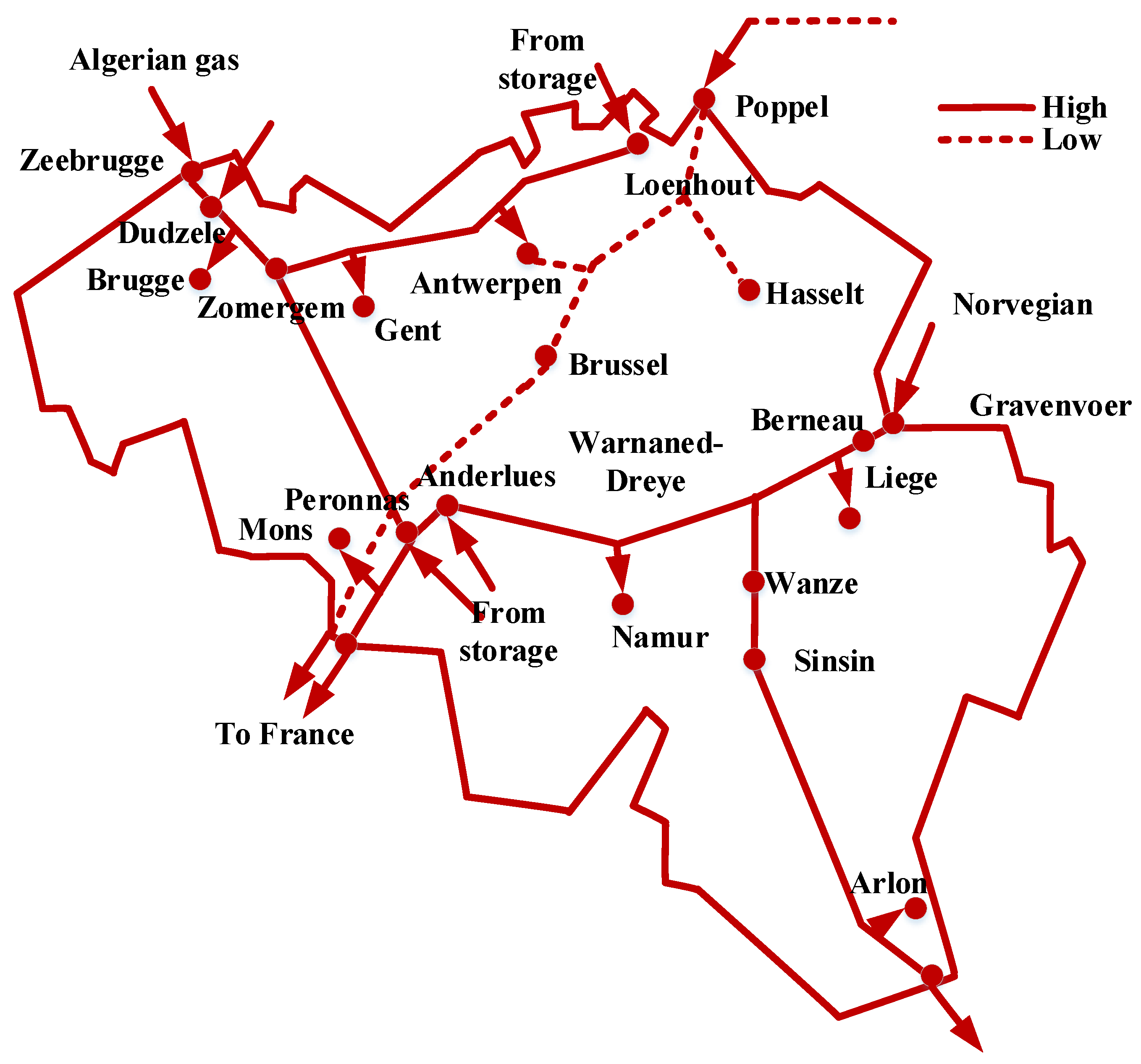
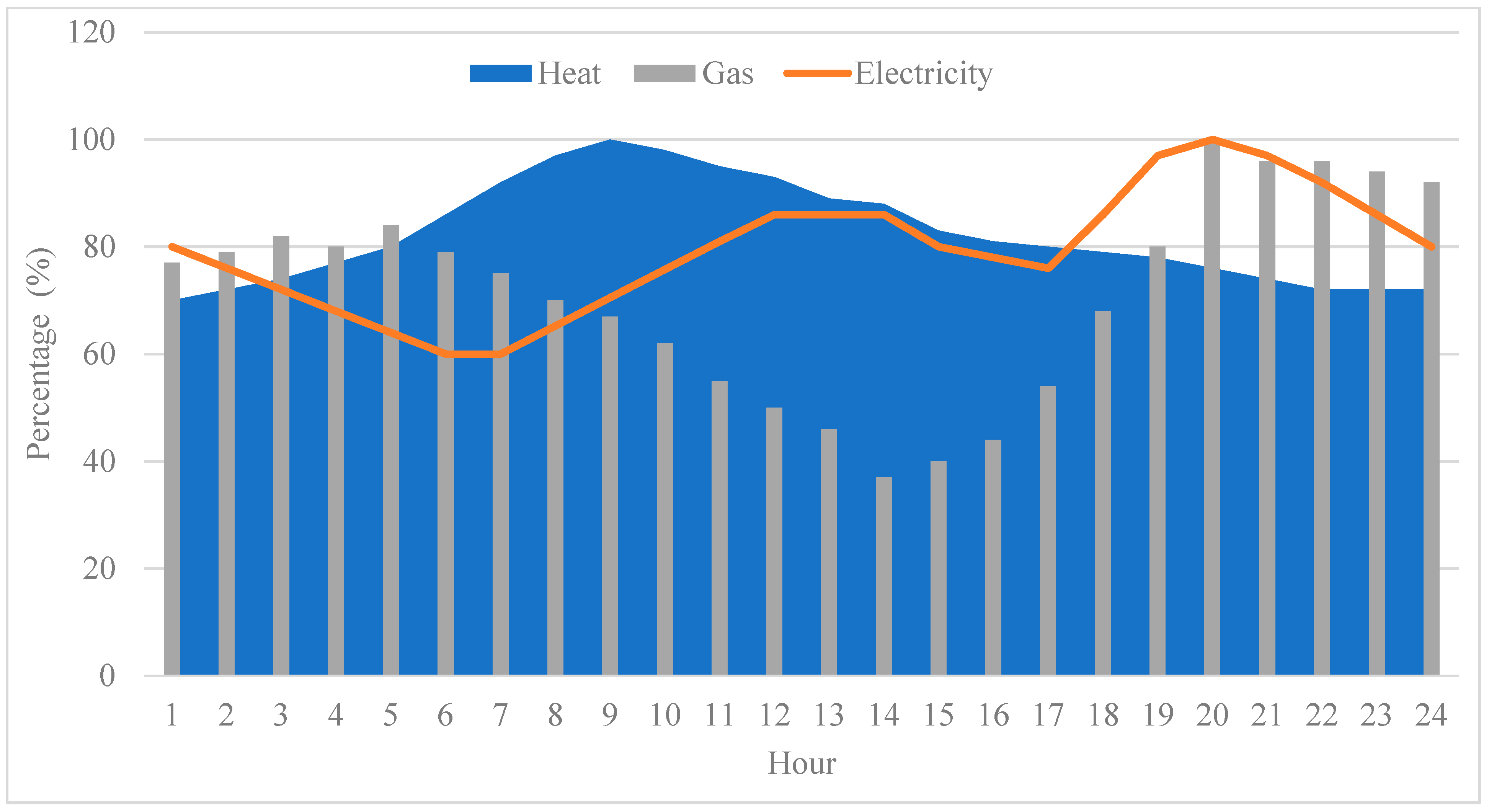
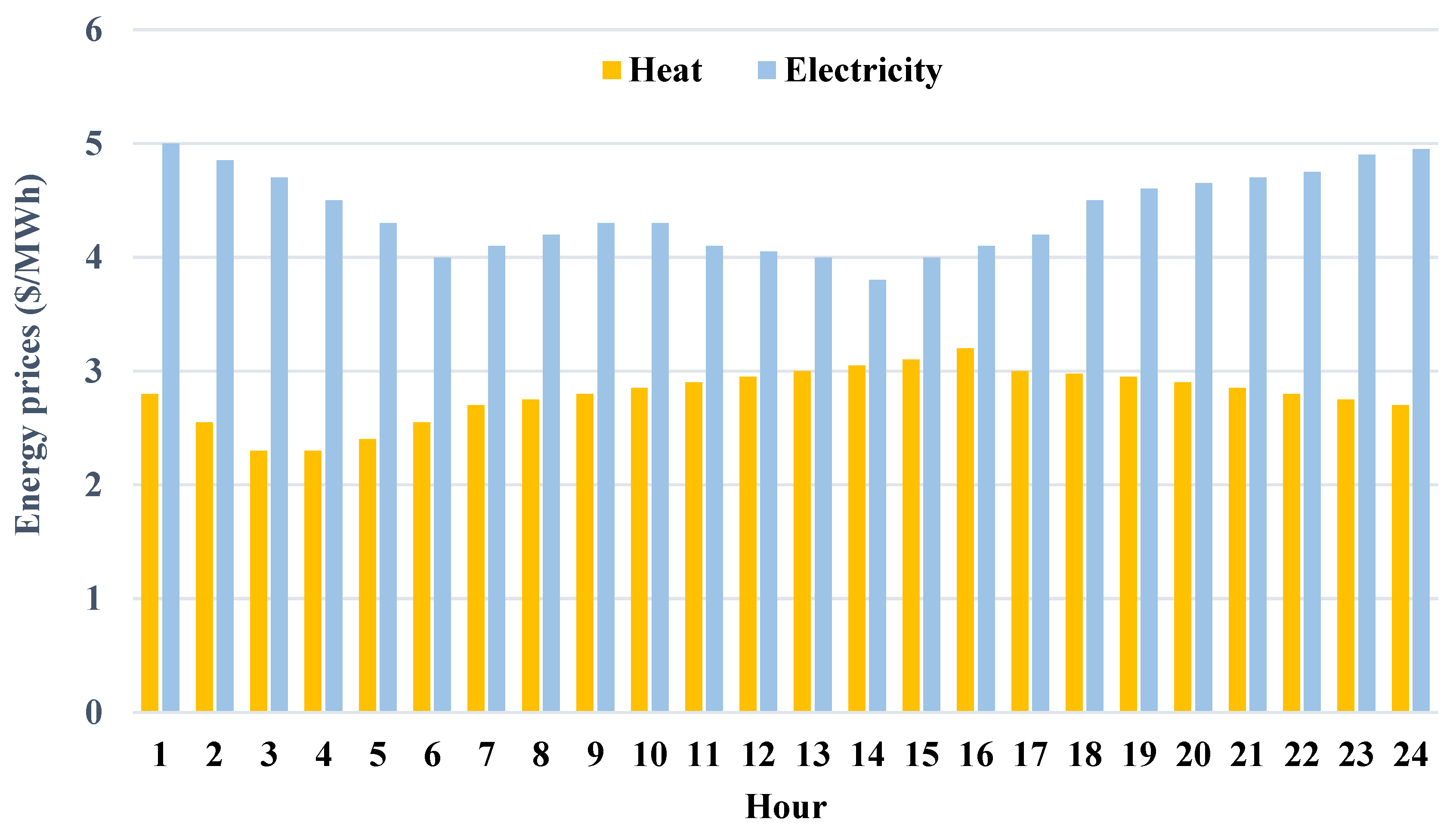
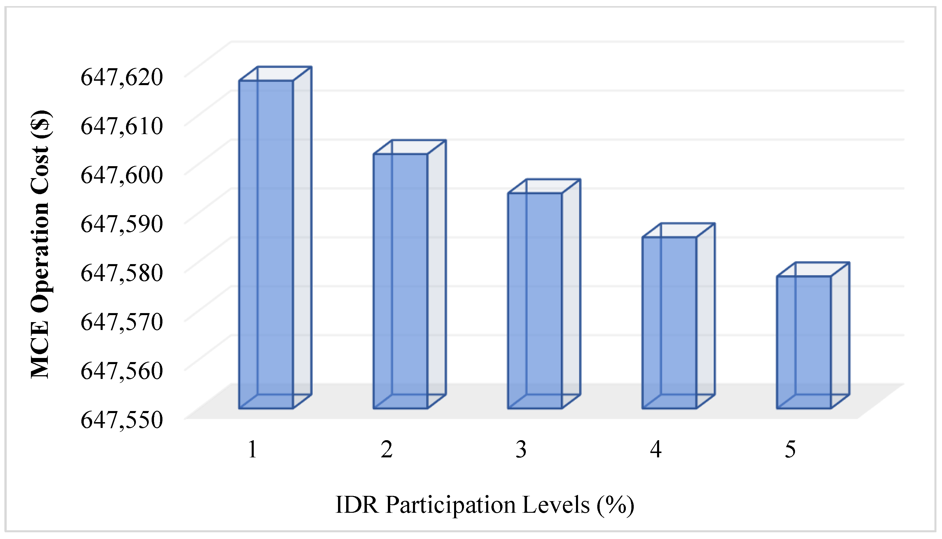
5. Numerical Evaluation

A numerical analysis of the suggested OEF taking into account DRP is presented in the following section. The outcomes examine the involvement of flexible energy users in the MCE’s OEF. The following part analyzes the advantages and features of the suggested OEF. The software and hardware needed are as follows: MATLAB (R2015a or later): Simulink and Simscape Power Systems; computer hardware requirements: processor: Intel Core i5 processor or equivalent; RAM: 8 GB or higher; hard disk: 500 GB or higher; graphics card: NVIDIA Quadro K4000 or equivalent; operating System: Windows 10. The proposed algorithm data are as below: primary learners: 10-20; count of population (NP): 50–100; teaching factor (α): 0.1–2; self-learning factor (β): 0.5–2; maximal count of iterations: 50–100.
For evaluating the suggested ITLBOA’s optimization capability, this paper compares the suggested algorithm with the outcomes of various non-linear optimization approaches. This paper then presents the outcomes of comparing the optimization algorithms for the MCE’s OEF. For traditional benchmark functions with different dimensions, Table 2 compares the suggested ITLBOA to a variety of different optimization algorithms. In this table, famous math benchmarks are deployed to measure the quality of the algorithms:
Schwefel: Schwefel’s function is a non-convex optimization benchmark used to test optimization algorithms. It is often used to evaluate the performance of global optimization algorithms as it is multimodal and has many local minima.
Ackley: The Ackley function is another non-convex optimization benchmark used to test the performance of optimization algorithms. It is often used to evaluate the performance of global optimization algorithms as it is multimodal and has many local minima.
Rosenbrock: The Rosenbrock function is a classic optimization benchmark used to test the performance of optimization algorithms. It is a convex optimization problem and is often used to evaluate the performance of local optimization algorithms.
Rastrigin: The Rastrigin function is a non-convex optimization benchmark used to test the performance of optimization algorithms. It is often used to evaluate the performance of global optimization algorithms as it is multimodal and has many local minima.
Griewank: The Griewank function is a non-convex optimization benchmark used to test the performance of optimization algorithms. It is often used to evaluate the performance of global optimization algorithms as it is multimodal and has many local minima.
In the experimental MCE system, there are 14-bus IEEE buses, 20-node gas networks, and 14-node heat networks [22,23]. In the sample MCE system, there are 2 electrical gas compressors, 5 boilers, 2 gas generators, 4 CHP units, 5 electric pumps, and direct links to gas, electrical power, and heat. Figure 1, Figure 2 and Figure 3 show a schematic diagram of sub-networks for the electrical network (Figure 1), gas network (Figure 2), and heat system (Figure 3). The integrated testing system considers four industrial IDR users as energy hubs, including flexible electricity and heat loads. Variables have the following minimums and maximums: V = [ 0.9 ,   1.1 ] pu, pressures = [ 5 ,   80 ] bar, supply temperatures [ 130 ,     110 ] 40 ° C , and return temperatures [ 55 ,     40 ] 40 ° C . Coefficients of heating ratio curves for gas-powered generators are a g e n = 0.008 ,   b g e n = 4 ,   c g e n = 150 ,   d g e n = 15 , and e g e n = 0.5 . Cost factors are u f u e l = 0 , v f u e l = 0.14126  $/m3, and v f u e l = 0 . of the gas. The information needed to optimize the proficiency of the integrated system is illustrated in Table 3. Table 4 provides the technical features of the three systems of the integrated system. For the ITLBOA algorithm, the size of the population is 80 and the overall number of iterations is 500. Flexible users’ shift of energy is limited to 25% of every hub’s energy demand. Figure 4 shows electricity and heat demand percentages for the integrated hubs over a 24 h period. Table 5 shows the interdependencies between the three heat, electricity, and gas systems within IDR hubs.
Figure 5 shows the power prices of the DRP per hour. Specifically, every hub’s needs are met by its devices or via the transmission sub-network within the MCE systems. When the hubs’ production power exceeds their loads, the excess energy is delivered to the associated network. An integrated system’s OEF problem poses a computational challenge due to the large-scale nature of gas, electricity, and heat sub-networks. It is, fortunately, possible to significantly minimize this problem with the suggested highly efficient approach. Since the proposed approach utilizes a combination of optimization techniques and machine learning algorithms to identify the optimal energy flows in the MCE system, it is capable of providing an accurate solution to the OEF problem while also reducing the computational complexity of the problem. Furthermore, the use of machine learning algorithms allows the system to adapt to changes in power prices and adjust the optimal energy flows accordingly. In addition, the proposed approach can be used to identify the most cost-effective energy sources for each hub in the MCE system, thus allowing for the most efficient use of energy resources. In the suggested OEF approach, the inverse of a variable Jacobian is not used for all iterations, as in Newton–Raphson approaches [24]. In addition, the holomorphic approach to address electric power flow can achieve a viable solution when all viable solutions exist; holomorphic methods do not require a primary guess of the system [25].
The holomorphic approach to addressing electric power flow in power systems is a mathematical approach that uses holomorphic functions to solve the equations of power flow in a power system. This approach is based on the fact that the power flow equations can be written as a set of holomorphic functions. This approach is advantageous because it allows for the solution of the equations without having to resort to numerical methods, which can be time-consuming and difficult to implement. Additionally, holomorphic functions can be used to analyze system behavior under different operating conditions, providing a more detailed understanding of system dynamics. This approach is also useful for detecting and diagnosing faults in power systems as it allows for the identification of potential issues that may not be visible with other methods. The main advantages of this method over the Newton–Raphson method are as below:
The holomorphic approach provides an exact solution to the power flow equations, while the Newton–Raphson method only provides an approximate solution.
The holomorphic approach is computationally efficient and does not require any iteration, while the Newton–Raphson method requires multiple iterations to reach a solution.
The holomorphic approach is more accurate as it takes into account the non-linearity of the power flow equations, while the Newton–Raphson method is based on linear approximations.
Figure 6 depicts the impact of DRP on the performance of the OEF of the experimental MCE system. According to the figure, the IDR program for the MCE systems reduces operational costs. The figure shows that with the greater flexibility of users’ involvement, the operational costs of the system are significantly decreased. A direct control method allows the ISO for managing flexible heat and electrical loads by means of an acceptable level of user involvement [26]. Incentives must be paid by the ISO to flexible users, though.
The load duration curves for the power and heating sub-systems in the presence and sans of the DRP are presented in Figure 7. To meet the heating and electricity needs of IDR users during peak times, the ISO consumes gas through CHP and hub boilers. The overall electrical loads of the system including and excluding the DRP during 24 h are shown in Figure 7a. The figures indicate that the total system electrical loads are decreased within peak durations. As a result of the DRP, the electrical load shape is better balanced as well. Due to the DRP per hour, the heat and electricity peak loads are shifted to times in which the price of providing electricity and heat is lower [27,28,29]. The DR led to a decrease in peak loads and a smoothing of the load curve of the heating system in Figure 7b.
For the purpose of investigating the DRP, three sub-networks were examined. Figure 8 shows the overall electrical power generated by generators in the MCE system in the presence and absence of DRP. The figure shows the reduction in electrical power generated by generators in the MCE in the presence of DRP.
Figure 9 shows the overall heat produced by the MCE system including and excluding DRP. The integrated heat DRP reduces the overall heat generated outside the energy hubs in the MCE. Heat network efficiency is improved by the DRP.
The overall gas produced by the system from the outside DR hubs in the presence and sans of DRP is depicted in Figure 10. A higher amount of gas is produced by the system in the presence of the DRP. This is because, in the DR hubs, equipment that is interdependent like CHPs and boilers consumes greater quantities of natural gas to provide both electricity and heat. Despite this, the overall operational prices of the multi-energy carrier system decreased because gas has a lower cost compared to various energy sources.
The losses of the networks in the presence of DRP and in the absence of DR in the two systems are depicted in Figure 11. It is concluded that the use of DRP diminishes electrical losses. Furthermore, if the DRP is incorporated into an integrated system, the overall heat loss decreases. In view of the assumption that the gas network is zero-loss, no gas loss is considered.
Figure 12 illustrates the change in nodal operations of the integrated network. When DRP is used, nodal voltages on the electrical system tend to be nearer the optimum voltage (1 pu), and such values tend to be near their maximum or minimum levels when not using DRP. Gas network nodal pressures in the absence of DRP outcomes are similar to those obtained in the presence of DRP outcomes. Gas network nodal operation is not affected significantly by flexible electricity and heat demands. According to Figure 12c, the nodal supply temperatures of the heating system in the absence of DRP tend to be closer to the maximum and minimum bounds than when DRP is utilized.
This paper compares the outcomes of the algorithm to the outcomes of other optimizer schemes to evaluate how the ITLBOA affects the OEF of the MCE experimental system. Table 6 illustrates this analysis.

6. Conclusions

The goal of the study was to peruse the involvement of integrated flexible users, a particular type of demand-side management activity, in MCE systems such as electricity, heat, and gas. This will be beneficial for both the energy provider and the customers as it will reduce the cost of energy. In addition, the coordination of multiple energy carriers will also help to reduce the environmental impact of energy production and consumption. This is because the coordination of multiple energy carriers will lead to more efficient use of energy, which will reduce the amount of energy wasted. This, in turn, will reduce the amount of greenhouse gases released into the atmosphere. Finally, the integration of multiple energy carriers will also make the energy system more resilient as it will be better able to cope with unexpected energy demand changes. An OEF scheme of the multi-power carrier system has been used for determining DR hubs’ impact. The OEF scheme considers electrical as well as heat loads in real time. The MCE is operated by elastic energy users. With the developed OEF scheme, electric, gas, and heat networks can be coordinated with industrial DR hubs while taking network security into consideration. Energy demand curves are smoothed by flexible energy users based on simulation outcomes. In addition, flexible energy users decrease the overall operational costs for integrated multi-power carrier systems. In addition, as the number of flexible electric and heat users increases, multi-energy carrier system operation prices decrease even further. As the number of flexible users in the system increases, DRP’s impact will become more evident.

Author Contributions

Conceptualization, T.C., L.G., S.I., M.J., M.A.E.-M., M.S. and S.G.A.; Methodology, S.I.; Software, S.I.; Validation, L.G., M.J. and M.S.; Formal analysis, T.C., L.G. and M.S.; Investigation, M.J.; Data curation, S.G.A.; Writing—review & editing, T.C., L.G., S.I., M.J., M.A.E.-M., M.S. and S.G.A.; Visualization, M.A.E.-M. All authors have read and agreed to the published version of the manuscript.

Funding

This research was funded by King Saud University through Researchers Supporting Program number (RSPD2023R704).

Institutional Review Board Statement

Not applicable.

Informed Consent Statement

Not applicable.

Data Availability Statement

Not applicable.

Acknowledgments

The authors present their appreciation to King Saud University for funding this research through Researchers Supporting Program number (RSPD2023R704), King Saud University, Riyadh, Saudi Arabia.

Conflicts of Interest

The authors declare no conflict of interest.

Abbreviations

DRPDemand response programOEFOptimal energy flow
ITLBOAImproved teaching–learning-based optimization algorithmCHPCombined heat and power
GTGas turbineEBElectric boilers
PVPhotovoltaicP2GPower-to-gas
WTWind turbineGSGas storage
MESMulti-energy systemDRDemand response
IGEHSIntegrated gas, electric, and heat systemCCGColumn-and-Constraint Generation
RERenewable energyMCEMulti-carrier energy
DSEDemand-side energyIDRIntegrated disaster response
ISOIndependent system operator

Nomenclature

VariableDefinition
U q , f u e l ,   V q , f u e l ,   W q , f u e l Fuel price’s ratio ($/ton)
τ q , f u e l Amount of fuel type consumed
L e , o u t , r t / L h , o u t , r t Output electrical/heat energy of every hub from the demand side (MW)
P E , j g e n Generators’ production active power (MW)
P m i n , j g e n / P m a x , j g e n Minimum/maximum generators’ production active power (MW)
Q E , j g e n Generators’ production reactive power (MVAR)
Q m i n , j g e n / Q m a x , j g e n Minimum/maximum generators’ production reactive power (MVAR)
V i ,   V j Voltage of the node in the system (pu)
ϕ H c h p CHP heat production (MW)
ϕ H b o i l e r Boiler heat production (MW)
T s , j c h p Initial temperatures of the CHP (K)
T s , j b o i l e r Initial temperatures of the boiler (K)
| P E ,   i j l i n e | Transmission flow of electrical line
| F G ,   i j l i n e | Transmission flow of gas line
| H ,   i j l i n e | Transmission flow of heat line
H r d a y Entire amounts of heat energy demand of the hub per day (MW)
E r d a y Entire amounts of electrical energy demand of the hub per day (MW)
F g · k Gas transmission from node g t h to k t h ( m 3 / d a y )
F g · L Gas demand at node ( m 3 / d a y )
F g · S Gas injection via node g t h  ( m 3 / d a y )
F g C H P / F g c o m p / F g b o i l e r CHP/turbo-compressor/boiler consumption gas ( m 3 / d a y )
m ˙ H b o i l e r / m ˙ H C H P Boiler/CHP ’s mass flow ratio ( k g / s )
m ˙ o u t / m ˙ i n Output/input mass flow via a pump ( k g / s )
m h b ˙ Mass flow via the pipeline among node h t h and b t h   ( kg / s )
m ˙ H H P Heat pump’s mass flow (kg/s)
m ˙ H l o a d Heat load’s mass flow (kg/s)
T e n d End of the pipeline’s temperature ( K )
T s t a r t Beginning of the pipeline’s temperature ( K )
l Heat pipeline’s length (km)
η c h p / η c o m p / η H P Efficiency of the CHP/compressor/pump
D h b H , L Pipeline’s diameter (mm)
L h b H , L Pipeline’s length (km)
Θ h b H , L Pipeline’s friction ratio
ρ W Water density/ k g / m 3
T i n / T o u t Input/output mass flow’s temperature in a mixed node ( K )
P k , i n c o m p / P k , o u t c o m p Pressure of input/output gas compressor
Q i d e m / g e n / P i d e m / g e n Reactive/active power demand
Q i C H P / P i C H P Reactive/active power production of CHP
Q i S H Shunt capacitors reactive production (MVAR)
P i c o m p Consumed electric power via compressor (MVA)
P i p u m p Consumed power via heating pump (MVA)
H p Network’s pump head (m)
N E Number of electrical bus
θ i Voltage angle
Y i j Electrical transmission line admittance
N h Number of heat nodes
a b o i l , a b o i l Partial boiler ratios
h / e Incentive cost that operator should pay to the flexible Heat/electric customers ( $ )
Γ Heat transition ratio ( W / mK )
T g Temperature of ground ( K )
c p Specific heat of the water ( k J / k g K )
α g k c o m p / α g k c o m p / α g k c o m p Compressor consumption ratio
γ G Gas’s gravity ratio
λ G Natural gas specific heat proportion
E p Gas pipelines’ absolute rugosity ratio ( m m )
L g k Length of pipeline (km)
Z Gas’s compressibility at the gas flow’s temperature
T a Gas flow’s temperature ( K )
T 0 Base temperature, ( K )
P 0 Base pressure ( k P a )
P E C H P CHP’s active power ( M W )
P E H P Heat power’s electrical demand ( M W )
P E , g c o m p Power demand of compressor  ( M W )
ϕ h , l o a d Customer point’s heat energy demand ( MW )
ϕ h b Heat energy flow via the heat pipeline  ( MW ) .
a g e n , b g e n , c g e n , d g e n , e g e n Consumption ratios of generator
R g k G L Reynolds number
K h b H , L Pipe’s resistance ratio
D g k G L Pipeline diameter ( m m )
Π a g k Pipeline mean pressure ( k P a )
Π g , i n c o m p Compressor’s input pressure ( k P a )
Π k , o u t c o m p Compressor’s output pressure ( k P a )
H p g k Pipeline’s slope pipeline correction ( kPa 2 )
H gk comp Compressor ratio among g t h node and k t h node
F G G Consumption gas via gas-fired power agent ( m 3 / day )
F t P 2 G Gas generation of P2G agent ( m 3 / d a y )
ϑ h b H , L Flow velocity ( m / s )
ϕ H b o i l , m a a x Maximum heat production of boiler ( M W )
ϕ h d e m Demand for heat energy at h t h node ( MW )

References

  1. Huang, X.; Xu, Z.; Sun, Y.; Xue, Y.; Wang, Z.; Liu, Z.; Li, Z.; Ni, W. Heat and power load dispatching considering energy storage of district heating system and electric boilers. J. Mod. Power Syst. Clean Energy 2018, 6, 992–1003. [Google Scholar] [CrossRef] [Green Version]
  2. Wang, H.; Wang, B.; Luo, P.; Ma, F.; Zhou, Y.; Mohamed, M.A. State Evaluation Based on Feature Identification of Measurement Data: For Resilient Power System. CSEE J. Power Energy Syst. 2021, 8, 983–992. [Google Scholar]
  3. Askari, M.; Dehghani, M.; Razmjoui, P.; GhasemiGarpachi, M.; Tahmasebi, D.; Ghasemi, S. A novel stochastic thermo-solar model for water demand supply using point estimate method. IET Renew. Power Gener. 2022, 16, 3559–3572. [Google Scholar] [CrossRef]
  4. Belderbos, A.; Valkaert, T.; Bruninx, K.; Delarue, E.; D’haeseleer, W. Facilitating renewables and power-to-gas via integrated electrical power-gas system scheduling. Appl. Energy 2020, 275, 115082. [Google Scholar] [CrossRef]
  5. Song, Y.; Mu, H.; Li, N.; Shi, X.; Zhao, X.; Chen, C.; Wang, H. Techno-economic analysis of a hybrid energy system for CCHP and hydrogen production based on solar energy. Int. J. Hydrogen Energy 2022, 47, 24533–24547. [Google Scholar] [CrossRef]
  6. Ma, H.; Liu, Z.; Li, M.; Wang, B.; Si, Y.; Yang, Y.; Mohamed, M.A. A two-stage optimal scheduling method for active distribution networks considering uncertainty risk. Energy Rep. 2021, 7, 4633–4641. [Google Scholar] [CrossRef]
  7. AlHajri, I.; Ahmadian, A.; Elkamel, A. Stochastic day-ahead unit commitment scheduling of integrated electricity and gas networks with hydrogen energy storage (HES), plug-in electric vehicles (PEVs) and renewable energies. Sustain. Cities Soc. 2021, 67, 102736. [Google Scholar] [CrossRef]
  8. Gan-yun, L.; Bin, C.; De-xiang, J.; Nan, W.; Jun, L.; Guangyu, C. Optimal scheduling of regional integrated energy system considering integrated demand response. CSEE J. Power Energy Syst. 2021. [Google Scholar] [CrossRef]
  9. Gabrel, V.; Murat, C.; Thiele, A. Recent advances in robust optimization: An overview. Eur. J. Oper. Res. 2014, 235, 471–483. [Google Scholar] [CrossRef]
  10. Yang, N.; Liu, S.; Deng, Y.; Xing, C. An improved robust SCUC approach considering multiple uncertainty and correlation. IEEJ Trans. Electr. Electron. Eng. 2021, 16, 21–34. [Google Scholar] [CrossRef]
  11. Wu, G.; Xiang, Y.; Liu, J.; Shen, X.; Cheng, S.; Hong, B.; Jawad, S. Distributed energy-reserve co-optimization of electricity and natural gas systems with multi-type reserve resources. Energy 2020, 207, 118229. [Google Scholar] [CrossRef]
  12. de Souza Dutra, M.D.; da Conceição Júnior, G.; de Paula Ferreira, W.; Chaves, M.R. A customized transition towards smart homes: A fast framework for economic analyses. Appl. Energy 2020, 262, 114549. [Google Scholar] [CrossRef]
  13. Zhang, Y.; Ai, X.; Wen, J.; Fang, J.; He, H. Data-adaptive robust optimization method for the economic dispatch of active distribution networks. IEEE Trans. Smart Grid 2018, 10, 3791–3800. [Google Scholar] [CrossRef] [Green Version]
  14. Qaeini, S.; Nazar, M.S.; Varasteh, F.; Shafie-khah, M.; Catalão, J.P. Combined heat and power units and network expansion planning considering distributed energy resources and demand response programs. Energy Convers. Manag. 2020, 211, 112776. [Google Scholar] [CrossRef]
  15. Yang, S.; Tan, Z.; Liu, Z.; Lin, H.; Ju, L.; Zhou, F.; Li, J. A multi-objective stochastic optimization model for electricity retailers with energy storage system considering uncertainty and demand response. J. Clean. Prod. 2020, 277, 124017. [Google Scholar] [CrossRef]
  16. Abdallah, W.J.; Hashmi, K.; Faiz, M.T.; Flah, A.; Channumsin, S.; Mohamed, M.A.; Ustinov, D.A. A Novel Control Method for Active Power Sharing in Renewable-Energy-Based Micro Distribution Networks. Sustainability 2023, 15, 1579. [Google Scholar] [CrossRef]
  17. Lu, Q.; Guo, Q.; Zeng, W. Optimization scheduling of home appliances in smart home: A model based on a niche technology with sharing mechanism. Int. J. Electr. Power Energy Syst. 2022, 141, 108126. [Google Scholar] [CrossRef]
  18. Mokhatab, S.; Poe, W.A.; Mak, J.Y. Handbook of Natural Gas Transmission and Processing: Principles and Practices; Gulf Professional Publishing: Houston, TX, USA, 2018. [Google Scholar]
  19. Lamri, A.A.; Easa, S.M. Computationally efficient and accurate solution for Colebrook equation based on Lagrange theorem. J. Fluids Eng. 2022, 144, 014504. [Google Scholar] [CrossRef]
  20. Yang, J.; Zhang, N.; Botterud, A.; Kang, C. On an equivalent representation of the dynamics in district heating networks for combined electricity-heat operation. IEEE Trans. Power Syst. 2019, 35, 560–570. [Google Scholar] [CrossRef]
  21. Rao, R.V.; Savsani, V.J.; Vakharia, D.P. Teaching–learning-based optimization: An optimization method for continuous non-linear large scale problems. Inf. Sci. 2012, 183, 1–15. [Google Scholar] [CrossRef]
  22. De Wolf, D.; Smeers, Y. The gas transmission problem solved by an extension of the simplex algorithm. Manag. Sci. 2000, 46, 1454–1465. [Google Scholar] [CrossRef] [Green Version]
  23. Ceseña, E.A.; Mancarella, P. Energy systems integration in smart districts: Robust optimisation of multi-energy flows in integrated electricity, heat and gas networks. IEEE Trans. Smart Grid 2018, 10, 1122–1131. [Google Scholar] [CrossRef]
  24. Cui, X.; Liu, Y.; Yuan, D.; Jin, T.; Mohamed, M.A. A Hierarchical Coordinated Control Strategy for Power Quality Improvement in Energy Router Integrated Active Distribution Networks. Sustainability 2023, 15, 2655. [Google Scholar] [CrossRef]
  25. Shi, Y.; Hou, Y.; Yu, Y.; Jin, Z.; Mohamed, M.A. Robust Power System State Estimation Method Based on Generalized M-Estimation of Optimized Parameters Based on Sampling. Sustainability 2023, 15, 2550. [Google Scholar] [CrossRef]
  26. Jasim, A.M.; Jasim, B.H.; Flah, A.; Bolshev, V.; Mihet-Popa, L. A new optimized demand management system for smart grid-based residential buildings adopting renewable and storage energies. Energy Rep. 2023, 9, 4018–4035. [Google Scholar] [CrossRef]
  27. Jasim, A.M.; Jasim, B.H.; Aymen, F.; Kotb, H.; Althobaiti, A. Consensus-based intelligent distributed secondary control for multiagent islanded microgrid. Int. Trans. Electr. Energy Syst. 2023, 2023, 6812351. [Google Scholar] [CrossRef]
  28. Tan, H.; Yan, W.; Ren, Z.; Wang, Q.; Mohamed, M.A. A robust dispatch model for integrated electricity and heat networks considering price-based integrated demand response. Energy 2022, 239, 121875. [Google Scholar] [CrossRef]
  29. Duan, Q.; Quynh, N.V.; Abdullah, H.M.; Almalaq, A.; Do, T.D.; Abdelkader, S.M.; Mohamed, M.A. Optimal scheduling and management of a smart city within the safe framework. IEEE Access 2020, 8, 161847–161861. [Google Scholar] [CrossRef]
Figure 1. Diagram of the electrical system.
Sustainability 15 10481 g001
Figure 2. Diagram of the gas system.
Sustainability 15 10481 g002
Figure 3. Diagram of the heat system.
Sustainability 15 10481 g003
Figure 4. Percentage of heat and electricity requirements of the combined hubs over a day.
Sustainability 15 10481 g004
Figure 5. Energy prices of the DRP per hour.
Sustainability 15 10481 g005
Figure 6. Operating costs of the MCE system in the presence of DR involvement levels.
Sustainability 15 10481 g006
Figure 7. Load duration curves for the heat and electricity sub-systems including and excluding the DRP. (a) Overall power curve for MCE systems; (b) overall heating curve for MCE systems.
Sustainability 15 10481 g007aSustainability 15 10481 g007b
Figure 8. Overall electricity produced via the electrical system.
Sustainability 15 10481 g008
Figure 9. Overall heat produced via the heating system.
Sustainability 15 10481 g009
Figure 10. Overall gas produced via the gas system.
Sustainability 15 10481 g010
Figure 11. Altering in loss power in the presence and absence of DRP. (a) Power system; (b) heating system.
Sustainability 15 10481 g011
Figure 12. Altering in nodal operation in the presence and absence of DRP. (a) Electrical system; (b) gas system; (c) heat system.
Sustainability 15 10481 g012
Table 1. ITLBOA algorithm.
1. Setting up parameters: The   step   defines   the   primary   learners   X o l d , i ,   count   of   the   population   ( NP ) ,   teaching   factor   ( T F ) , self-learning  factor   ( S F ) and   maximal   count   of   iterations   ( G m a x ).
2. Primary
population:
The primary randomly selected population of each learner is created within its bounds, as shown below:
X o l d , i = X o l d , i m i n + r a n d ( 0 , 1 ) ( X o l d , i m a x X o l d , i m i n )
X o l d , i = [ P E , j g e n , ϕ H , j c h p , ϕ H , j b o i l , T s , j c h p , T s , j b o i l , H j c o m p , L e , o u t , r t , L h , o u t , r t ]
in   which   i = 1 ,   ,   D ;   X o l d , i m i n   is   the   minimal   bound   of   the   i t h   learner   and   X o l d , i m a x   is   the   maximal   bound   of   the   i t h learner.
3. Teacher
step:
The updated learner vectors are created via achieving the knowledge from the trained teachers within the step. The created updated vector can be defined as follows:
X n e w 1 , i = X o l d , i + D i f f M e a n
in   which   D i f f M e a n   i = r a n d i ( M n e w _   T F M i )
in   which   M i  shows the mean knowledge level of the learners at time  i and   M n e w  shows the predicted knowledge level of learners;  T F   shows   the   teacher   factor   deciding   the   amount   of   M i  to be  1  or  0   and   r a n d i  shows a randomly selected number between  0  and  1 .
In   addition ,   T F can be defined as follows:
T F = r n d [ 1 + r a n d ( 0 , 1 ) ]
4. Learner
phase using
self-learning capability:
During this step, the newly acquired knowledge level of the learners is improved (i) through interacting with their peers or (ii) their self-learning capability:
X n e w 2 , i = { X n e w 1 , i + r 1 ( X o l d , i X o l d , j ) + r 2 ( X t e a c h e r S F X o l d , i ) i f   f ( X o l d , i ) > f ( X o l d , j ) X n e w 1 , i + r 1 ( X o l d , j X o l d , i ) + r 2 ( X t e a c h e r S F X o l d , i ) i f   f ( X o l d , j ) > f ( X o l d , i )
in   which   r 1   and r 2     are   the   randomly   selected   numbers   between   [ 0 ,   1 ]   and   S F , the self-driven learning factor, which can be determined as follows:
S F = r n d [ 1 + r a n d ]
5. Analyze/
choosing:
The   newly   created   learner   vector   X n e w 2 , i   at   stage   4   competes   with   its   previous   individuals   X o l d , i on the basis of the below evaluation criteria:
X i 1 = { X n e w 2 , i           i f           f ( X o l d , i ) f ( X n e w 2 , i ) X o l d , i                                                                       o t h e r w i s e
6. The end: The   procedure   is   repeated   until   the   preset   G m a x is reached.
Table 2. Comparing outcomes of algorithms in benchmark testing functions.
Benchmark Test FunctionAlgorithms
ITLBOATLBOPSO
SchwefelMean 1.6 × 10 3   ±   57 3.7 × 10 3 ± 284 5.2 × 10 3 ± 374
Time (s)0.890.931.04
AckleyMean 7.3 × 10 17 ± 1 × 10 19 8.5 × 10 10 ± 2 × 10 9 5.9 × 10 6 ± 7 × 10 7
Time (s)0.910.931.04
RosenbrockMean 28.75 ± 0.4 68.6 ± 3.7 256.8 ± 6.9
Time (s)1.311.221.3
RastriginMean0 82.4 ± 4.3 163.7 ± 5.8
Time (s)1.161.111.23
GriewankMean0 6.7 ± 16 × 10 2 25.2 ± 8 × 10 1
Time (s)1.171.141.21
Table 3. Technical information about energy sources in the MCE.
Unit Boiler   of   h u b 4 Boiler   of   h u b 3 Boiler   of   h u b 2 Boiler   of   h u b 1 Slack Boiler
T m i n , s , j b o i l , C 115115115115115
T m a x , s , j b o i l , C 125125125125125
Φ H , j b o i l e r , m i n , MW 00000
Φ H , j b o i l e r , m a x , MW 555515
UnitCHP of h u b 4 CHP of h u b 3 CHP of h u b 2 CHP of h u b 1
T m i n , s , j c h p , C 115115115115
T m a x , s , j c h p , C 125125125115
Φ H , j c h p , m i n , MW 0000
Φ H , j c h p , m a x , MW 30303030
UnitGenerator 2Generator 1
Q m a x , j g e n , j 5080
Q m i n , j g e n , j 00
P m i n , j g e n , MW 1015
P m a x , j g e n , MW 80332.4
Table 4. Information about the sub-networks.
Heat system c p = 4182   kJ / kg   K ρ w = 960   kg / m 3 g = 9.81   kgm / S 2 H p = 100   m η H P = 0.65
U = 0.2   W / m   K η t c h p = 0.88 Φ H b o i l , m a x =   5   MW b b o i l =   0.822 a b o i l =   0.0169 T g =   10   ° C
Electrical system a c h p =   0.463 b c h p =   0.0491 c c h p =   4.49
d 1 c h p =   0.8 d 2 c h p =   0.6 e 1 c h p =   0.0736 e 2 c h p =   0.0845
Gas system G H V = 40.611   MBTU / m 3 ε G =   0.05 mm Z a =   0.8 γ G =   0.6106 λ G =   1.309
π 0 =   1.0133   bar T G =   281.15   k T 0 =   273.2   k η G C = 0.8
Table 5. MCE configuration.
DevicesGeneratorSlack GeneratorMoto-CompressorMoto-CompressorSlack Boiler
and Pump
Heat node----1
Power bus215330
Gas node19129183
DevicesIDR  h u b 4 IDR  h u b 3 IDR  h u b 2 IDR  h u b 1
Heat node131094
Power bus7172314
Gas node106715
Table 6. Algorithm outcomes of OEF for testing MCE systems.
Method of SolutionITLBOATLBOPSO
Overall
operational
costs ($)
Time, s426843114401
SD0.1370.3140.529
Worst647,871647,893647,912
Mean647,859647,878647,887
Optimal647,858647,876647,884
Disclaimer/Publisher’s Note: The statements, opinions and data contained in all publications are solely those of the individual author(s) and contributor(s) and not of MDPI and/or the editor(s). MDPI and/or the editor(s) disclaim responsibility for any injury to people or property resulting from any ideas, methods, instructions or products referred to in the content.

