Abstract
Based on balanced panel data from 30 provinces and cities (excluding Hong Kong, Macao, Taiwan, and the Tibet Autonomous Region) from 2016 to 2020, this article empirically analyses the spatial effect of green credit (GD) on air quality index (AQI) and the regulatory mechanism between them and explores the differences in the impact of GD on AQI by dividing China into regions in terms of geographical distribution, financial development level, and air quality level. The empirical results found that AQI depends on significant spatial characteristics. GD has a significant inverted U-shaped impact on AQI and is currently at the stage of suppressing air quality. The inverted U-shaped impact is more remarkable in the eastern region, in areas with poor financial development, in areas with poor air quality and GD has entered the stage of promoting air quality levels in the eastern regions, and in areas with good financial development. Environmental regulation has a negative moderating effect on the relationship between GD and AQI, which is less pronounced in eastern regions, in areas with poorly financial development, and in areas with better air quality.
1. Introduction
Since the Industrial Revolution, more and more global environmental problems have come to the fore along with the rapid economic development of countries around the world. Global warming, rising sea levels, carbon dioxide, sulphur dioxide, smoke emissions, and other issues seriously threaten the future of human society. According to data from the International Energy Agency, global carbon emissions have been increasing since 2010, and China has been the world’s largest carbon emitter for many years in a row. In order to reduce greenhouse gas emissions, President Xi Jinping proposed the “Carbon Peaking and Carbon Neutral” strategy (hereinafter referred to as “Double Carbon”) at the 75th UN General Assembly.
China’s Ministry of Ecology and Environment (MOE) released the “Communiqué on the State of China’s Ecological Environment in 2020”, which states that only 59.9% of the 337 cities at prefecture level and above in China met the standard. In order to improve urban air quality level and achieve healthy development of ecological civilisation, the 14th Five-Year Plan proposes the establishment of a sound environmental governance system and collaborative promotion to reduce emissions. People’s concern about environmental quality, especially air quality, is gradually increasing, so this paper chooses AQI to measure air quality in order to include public perception. At present, under China’s predominantly indirect financing system, green credit plays a central role in the green financial system. As the most important part of China’s green financial system, green credit guides the flow of funds to low-pollution and low-energy industries by transforming the traditional financing environment and reducing the intensity of air pollutant emissions, thus promoting the improvement of China’s air environment quality and high-quality economic development. According to statistics, in 2015, China’s sulphur dioxide, nitrogen oxide, and smoke (dust) emissions were, respectively, 18.591 million tons, 18.518 million tons, and 16.279 million tons, while emissions from industrial production accounted for 88.1%, 67.6%, and 83.6%, respectively, of these emissions. Industrial activities have seriously affected the atmospheric environment. In 2016, China’s industrial added value accounted for 30.87%, the balance of green credit was 7.51 trillion CNY, and the average AQI of Chinese provinces was 80.11. In 2020, China’s industrial added value accounted for 32.87%, with a green credit balance of 11.95 trillion CNY and an AQI of 67.72. During the period from 2016 to 2020, the proportion of China’s industrial output value continued to grow, which inevitably caused damage to the environment. At the same time, the balance of green credit continued to increase, AQI showed a downward trend, and air quality level had improved overall.
Because the property rights of environmental resources are not clear and a market-based mechanism cannot work, negative environmental externalities can only be dealt with through administrative regulation and internalization of externalities. The intervention of the government is often based on punishment after the event and leads to “government failure” due to its low efficiency and incomplete information. Better investment and financing instruments and policies are needed to replace the current mode of operation, and green finance with environmental protection at its core is essentially a market-oriented ecological compensation mechanism which can not only promote economic growth, but also lead to sustainable economic development and harmonious coexistence between humans and nature. Enterprises and financial institutions should actively fulfil their social responsibilities, strengthen their business ethics, support environmental protection and circular economy, and practise green finance. Therefore, in order to help enterprises to grasp the progress of green transformation and achieve low pollution production, as well as to help the government find green financial methods to improve atmospheric problems, examine the effects of current environmental controls in the carbon context, and promote social benefits and improve the quality of life of the general public, it is necessary to study the impact of green credit on air quality levels.
Is there a spatial characteristic of air quality? How effective is the policy of green credit in improving air quality? What is the moderating effect of the “dual carbon” context on the impact of green credits on air quality levels? Do such policy effects vary across regions? If so, what is the specific impact in different types of areas? By exploring the above issues in depth, we can enrich the theoretical content of green credit and air quality studies and find suitable financial methods and approaches to solve the current air pollution problem.
2. Literature Review
Scholars’ research on the relationship between finance and air pollution has become more comprehensive, mainly focusing on the following three points. Firstly, financial development reduces air pollution. The support of financial resources can alleviate production pressure, promote green technology innovation, and reduce emission of pollutants, thereby optimizing air quality, which is manifested as the “emission reduction effect” [1,2,3]. Secondly, financial development will exacerbate the deterioration of air quality. With the booming financial industry, when financial resources are efficiently allocated, the scale of production expands, which increases energy resource consumption and pollution emissions, manifesting as an “increasing effect” [4,5]. Thirdly, there is a non-linear relationship between financial development and environmental pollution. Financial development can lead to both technological innovation to reduce air pollution and the expansion of production which exacerbates air pollutant emissions. The non-linear relationship is just the result of the interaction between the “increase effect” and the “reduction effect” [6,7,8,9]. “As an innovative development of traditional finance, green finance can promote environmental improvement, combat climate change and use resources efficiently”. Cowan [10] pointed out that green finance is a brand new path to combating environmental pollution and improving environmental quality, and based on this, he proposed that fund flow is a key research element of green finance, which can effectively reduce carbon emissions [11] and reduce air pollution emissions by promoting the energy-saving transformation of traditional industries and supporting the development of green industries [12,13,14]. “As an important part of green finance, green credit improves environmental pollution by providing loan support to green businesses and limiting loans to high energy-consuming and polluting enterprises.” Labatt et al. [15] argued that green credit, as an important element of the green financial system, is an important financial instrument to control environmental pollution and avoid environmental risks. Zhang et al. [16] used a panel dataset of 945 A-share listed companies from 30 provinces from 2004 to 2017 to construct a difference model to study changes in corporate investment and financing behaviour, and the results showed that green credit can reduce sulphur dioxide and wastewater emissions. Pan [17] used the Opinions on Implementing Environmental Protection Policies and Rules and Preventing Credit Risks in 2007 as a quasi-natural experiment to test the emission-reduction effect of credit instruments on highly polluting enterprises with the DID method; the results showed that green credit significantly inhibited the pollution emissions of highly polluting enterprises, and this inhibiting effect was mainly observed in large enterprises and areas with lower pollution levels and less regional development pressure. Kumar et al. [18] used the scientometric approach of VOSviewer to show the exact situation and trends in the field of “air pollution exposure and health”. It was found that health effects due to air pollution exposure has been the most researched topic in the last 5 years. There is the potential to change the structure of research networks and work in both developing and developed countries in order to make progress in the area of air pollution and strengthen measures of exposure and health. This means that the focus of scholars on air pollution is gradually shifting towards human health. AQI not only represents air pollution levels but also includes the public’s assessment of air quality based on how their health is affected. Qiao [19] constructed a bidirectional random effect model based on provincial AQI data from 2013 to 2017 to study the impact of green credit on air quality. The results show that green credit can significantly improve the air quality of each province. Mahato et al. [20] found a strong correlation between BC and PM2.5 concentrations during an assessment of black carbon (BC) and PM2.5 concentrations at municipal solid waste incineration sites in Jamshedpur. This suggests that municipal domestic waste also has a significant impact on air quality and that improvement of the atmospheric environment is urgent. We need financial measures to improve air quality levels. Regarding the study of “dual carbon” and green credit, Zhao et al. [21] constructed a model of double oligopoly competition in the ride-hailing procurement market in the context of “carbon peaking”, taking into account government subsidies and customers’ green preferences, and considered the reality of green credit policies and the general case of the ride-hailing procurement market to provide management suggestions for the sustainable development of the ride-hailing procurement market. He et al. [22] constructed a Richardson model based on data from 141 listed renewable energy companies in China to measure their investment efficiency. The results indicate that the overall development of green finance in China has suppressed the issuance of bank loans while also inhibiting the improvement of investment efficiency in renewable energy. This indicates that green finance reduces the improvement of energy efficiency and is not conducive to the implementation of energy-saving and carbon-reduction policies. In terms of the relationship between air pollution and carbon emissions, Zeng et al. [23] used the Kaya constant equation and LMDI decomposition model to analyse the synergistic emission reduction impacts and indirect drivers between air pollution and carbon emissions based on inter-provincial panel data in China from 2005 to 2019. The results show that the drivers of the synergistic effect between air pollution and carbon emissions are mainly energy efficiency and industrial structure, and that strengthening environmental regulation can improve the synergistic emission reduction impact of air pollutants and carbon emissions in the transport sector.
A review of the available literature reveals that while scholars are now well-established in their research on traditional finance and air pollution, there is less literature on green credit and air pollution and even less literature on green credit and air quality based on AQI. This paper empirically analyses the impact of green credit on air quality and the adjustment mechanism in the context of dual carbon based on balanced panel data of 30 Chinese provinces (excluding Hong Kong, Macao, Taiwan, and Tibet) from 2016 to 2020, as well as the specific differences of this impact in different regions, and proposes corresponding countermeasures.
3. Materials and Methods
3.1. Variables and Data
3.1.1. Dependent Variable
At present, scholars mostly use PM2.5 as a measure of air quality when studying air pollution and rarely take AQI into account, leading to incomplete measurement. In 2012, the Chinese government issued the Ambient Air Quality Standard (GB3095-2012), and AQI can be used to quantitatively evaluate air quality conditions more comprehensively. The results will also be closer to the public’s true perception. However, as the greater the AQI, the more serious the air pollution level and the worse the air quality level, this paper selects AQI as an inverse proxy for air quality, denoted as aqi. To prevent the effect of heteroskedasticity on the experimental results, AQI was logarithmised.
3.1.2. Core Explanatory Variable
Due to the lack of provincial data on the green credit balance of commercial banks and the balance of energy conservation and environmental protection loans, and because the data on the share of bank loans in industrial pollution control funds have not been counted since 2010, taking into account the completeness of the data and referring to Xie et al. [24], this paper selects the proportion of interest expenditure of non-six high energy consuming industries to measure green credit indicators (gd).
3.1.3. Adjustment Variable
Environmental regulation (ers): In the context of the dual carbon target, in order to explore the impact of environmental regulation on air quality, we, referring to the definition of constraint indicators in the national economic and social development plan and the practice of Mao et al. [25], weighted the binding indicators “reduction in energy consumption per unit of GDP” and “reduction in carbon dioxide emissions per unit of GDP”, and then, using the weighted energy-saving and carbon-reduction binding intensity index as an environmental regulation indicator. The specific formula is as follows:
where the subscript denotes province , denotes year , and denotes the lagged period of the corresponding variable; is total energy consumption (million TCE), is gross domestic product (billion CNY), and is total carbon dioxide emissions (million tons). If the value of the environmental regulation is greater than 1, it means that the intensity of the current energy saving and carbon reduction constraint is less than that of the previous period; if the value is less than 1, it means that the intensity of the current energy saving and carbon reduction constraint is greater than that of the previous period; if the value is equal to 1, it means that the intensity of the current energy saving and carbon reduction constraint is equal to that of the previous period. Since intensity is the opposite of the intensity index, the reciprocal of the energy saving and carbon reduction constraint intensity index is used as the energy saving and carbon reduction constraint intensity (ers) for ease of interpretation later on.
3.1.4. Control Variables
In order to avoid estimation bias by missing variables, referring to relevant theories of environmental pollution and drawing on research results from others, this paper selects indicators to control for social attribute variables affecting air quality from four perspectives: urbanisation, economic development, greening level, and industrial structure, where urbanisation is measured by ratio of urban population to total population (urb) (%); economic development is characterized by gross domestic product per capita (regdp) (CNY/person); industrial structure is measured by the proportion of secondary industry in GDP (is) (%) [26]; and greening level is measured by the formula that urban green space divided by resident population multiplied by 100 (green) (hundred hectares/person) [27]. In order to avoid the influence of heteroskedasticity, regdp is treated logarithmically in this paper.
3.1.5. Data Sources
Based on the provincial perspective, this paper selects panel data from 30 provinces in China from 2016 to 2020 (some indicators are seriously missing in Hong Kong, Macao, Taiwan, and the Tibet Autonomous Region, so they are excluded) as the research sample for the sake of data availability and completeness, and the missing data are filled in by linear interpolation. green credit data were selected from the China Industrial Statistics Yearbook, while air quality data were obtained from the China Air Quality Online Monitoring and Analysis Platform (https://www.aqistudy.cn/historydata/, accessed on 13 September 2022), and other data were obtained from the China Energy Statistics Yearbook, China Industrial Statistics Yearbook, the China Statistical Yearbook, and the statistical yearbooks of various provinces and cities in various years. The specific descriptive statistics are shown in Table 1. From the results, it is clear that the variance of each variable is small, indicating that the sample is relatively evenly distributed and there is no problem of extreme values. When provinces are categorised by geographical location, green credit is higher in the eastern regions than in the central and western regions, but air quality levels are relatively poor. When provinces are categorised by financial market level, higher-level areas have higher levels of green credit compared to low-level areas, but poorer levels of air quality. When provinces are categorised by air quality level, green credit is lower in areas with good air quality compared to areas with poor air quality. We can find that there are significant differences in the levels of green credit and air quality in areas of different geographical location, different levels of financial development, and different levels of air quality, so heterogeneity needs to be tested in subsequent studies.

Table 1.
Descriptive statistics.
As can be seen from Figure 1, nationally, during the five-year period from 2016 to 2020, the annual average value of AQI in China shows an “M” trend of “up–down–up–down”, with an overall downward trend. The percentage of these years with an annual average AQI value of excellent, respectively, is 6. 67%, 6.67%, 10%, 10%, 13.33%. This share rises slightly from 2019 and continues to rise in 2020; the percentages of light pollution for each year are 20%, 20%, 0%, 10%, and 0%, and the trend is an inverted “N” shaped curve of “down–up–down”. By region, the five-year trends in air quality in China’s eastern, central and western regions, low financial development regions, and high financial development regions are consistent with the national trend, all showing an “M” pattern, with a clear downward trend in 2018. In particular, the air quality conditions in the eastern region are consistently worse than those in the central and western regions, while the air quality gap between the high financial development area and the low financial development area narrowed each year over the five-year period.
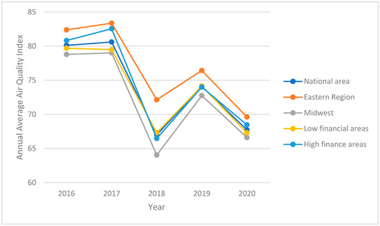
Figure 1.
Map of air quality trends.
3.2. Econometric Model
Considering the imbalance of air pollution in different countries and regions, the air quality level of a region may be affected by neighbouring regions. Therefore, this paper uses a spatial econometric model to explore the spatial effect of green credit on air quality index.
3.2.1. Weight Matrix
The spatial weight matrix is mainly used to quantitatively measure the closeness of the spatial connections between the variables on the region, which can effectively measure the corresponding spatial effects, which is crucial in the spatial model analysis. The spatial weight matrix is a matrix that represents the set of neighbours of each spatial unit, which specifies the connectivity between spatial units. Currently, available spatial weight matrices include neighbourhood matrices, spatial geographic distance matrices, economic distance matrices and economic–geographic nested matrices. The details of how these are constructed are shown below.
The adjacency matrix is assigned according to whether the spatial units are adjacent to each other and is constructed as follows.
The spatial geographic distance matrix is set based on the geographic distance of the spatial units and is calculated as follows.
where denotes the Euclidean straight-line distance between the central locations of province i and province j.
The economic distance weight matrix is set using the economic gap between regions, based on the level of economic development between regions, and is constructed in the following way.
where and are the GDP per capita of province and province between 2016 and 2020, with the inverse of the difference in means set as the weights.
The economic geographical weight matrix takes into account both the effects of economic and geographical interaction by organically combining the economic distance matrix with the spatial geographical matrix, which is constructed in the following way.
With reference to most scholars, this paper chooses the spatial adjacency matrix as the baseline spatial matrix. To further test the robustness of the effect of green credit on air quality, this paper considers the influence of different spatial weight matrices on the estimation results and constructs a spatial geographic matrix and a spatial economic geographic matrix.
3.2.2. Spatial Model
Prior to modelling, we need to make model assumptions, the conditions of which are shown below.
(1) The spatial error model (SEM) assumes the condition that there is an interaction between regions, and that this effect is realized through the error term.
(2) The spatial lag model (SAR) assumes the condition that there is an interaction between regions, and that this is achieved through the independent variables.
(3) The spatial Durbin model (SDM) assumes that there are interactions between regions, and that this is achieved through the independent and dependent variables.
Referring to Wang et al. [28], the model was constructed in the following specific form by considering the quadratic relationship between economic growth and environmental pollution in the EKC.
The SEM assumes that spatial correlations between areas arise primarily from spatial correlations between random disturbance terms and constructs the model in the following specific form.
where represents the air quality index of province in year ; denotes the level of green credit, and represents the quadratic side of the level of green credit; represents other control variables, including economic development (), urbanisation level (), industrial structure (), and greening level (). represents the regression coefficient of each explanatory variable; is an element on the standardised spatial weight matrix W, representing the strength of spatial association between regions; represents the spatial autocorrelation error term, denotes the spatial autocorrelation coefficient, and represents the random disturbance term.
Further considering the impact of the “dual carbon” context on green credit and air quality, environmental regulation () is added to the model as a moderating variable as well as an interaction term between green credit and environmental regulation) (). Referring to Wu et al. [29], the model is constructed in the following form:
where denotes the level of environmental regulation and is the interaction term between environmental regulation and green credit, and the other variables are consistent with the above.
For comparison, both a spatial lag model and a spatial Durbin model were constructed.
SAR assumes that the spatial correlation between regions stems primarily from the spatial correlation between the explanatory variables and constructs the model in the following specific form.
where denotes the spatial autoregressive coefficient, is an element on the normalised spatial weight matrix W, denotes the spatial lagged dependent variable, and denotes the random disturbance term.
Taking into account the effect of the dual carbon background, the model was constructed as follows.
SDM assumes that the spatial correlation between regions stems primarily from the spatial correlation between the explanatory and explanatory variables, constructing the model in the following specific form.
where represents the stochastic perturbation term. Taking into account the effect of the dual carbon background, the model is constructed as follows.
4. Results and Discussion
4.1. Spatial Effect Analysis
This paper uses the Stata17.0 software program to construct the SAR, SEM, and SDM, using short panel data with “large N and small T”. Regression analysis was conducted on the data from 2016 to 2020, and the regression results are shown in Table 2. In order to control for possible heteroskedasticity in the model, robust standard errors are used in the spatial regression process in this paper. As can be seen from the table, in terms of spatial effects, the spatial regression coefficient and spatial error coefficient among the three models are significantly positive and all pass the 1% significance test, indicating that there is a significant positive spatial correlation between provincial air quality and that the air quality of a region is subject to shocks and disturbances from neighbouring regions, and therefore the influence of spatial externalities should not be skimmed when studying the relationship between green credit and air quality. This also indirectly demonstrates the necessity of using spatial econometric models. The regression results of the SAR, SDM, and SEM models without control variables are shown in Table 2 for Models I, IV, and VII respectively, representing the total effect of green credit on AQI under the three models. We can see that the relationship between green credit and AQI shows a significant inverted “U” shape, that is, the air quality situation shows a “deterioration–improvement” development trend as the level of green credit increases. When the level of green credit is low, AQI tends to rise as the level of green credit increases and air quality deteriorates; when the level of green credit crosses the inflection point, AQI decreases as the level of green credit increases, and the air quality level gradually improves. As an important part of green finance, green credit is an important contemporary tool for achieving ecological environmental protection. Specifically, by directing the flow of bank funds, green credit increases support for loans to enterprises engaged in ecological protection and green production; furthermore, it promotes the development of green productivity and plays a role in environmental protection. Given the non-linear relationship between green credit and air quality in the empirical evidence, the SEM calculated the inflection point to be.0.5667, which is greater than the mean value of 0.492, indicating that most regions have not crossed the inflection point and the impact of green credits on air quality is still in the suppression stage which is not consistent with the study by Qiao [19], who confirmed that green credit directly improves air quality. A possible reason for this is that the local government did not invest in green credit or support green industries enough, which meant the capital-borrowing needs of customer groups were not met, causing the enterprises to turn to increased investment in non-green industries, further polluting the environment and worsening air quality. With the increase of green credit, enterprises are profitable and gradually increase their investment in green industries and green production. Thus, the increase of green credit can significantly reduce the average concentration of each pollutant in the atmosphere, reduce air quality index, and achieve the goal of improving air quality. This also demonstrates the validity of the national strategy of “utilizing the financing-oriented role of green finance”. Models II, V, and VIII are the regression results of the SAR, SDM, and SEM, respectively, after the addition of control variables. The positive and negative coefficients and significance of the core explanatory variables remain unchanged, further indicating the robustness of the inverted U shape of green credit and AQI.
Table 2.
Comparison of the three models.
Models III, VI, and IX are the regression results of the SAR, SDM, and SEM models with the introduction of the moderating variables and the interaction term between green credit and moderating variables, respectively. Compared to the regression results without the moderating terms and their interaction terms, the absolute values of the coefficients of the quadratic terms of green credit increase in all three models, and the coefficients of the environmental regulation and interaction terms are all significant at the 5% level, indicating that the moderating role of environmental regulation in the impact of green credit on air quality in the context of dual carbon is significant and cannot be ignored. In the LM test, we can see that SEM has the best test results in both states with control variables and with moderating variables, and it also has the relatively better regression results. From the results of the likelihood ratio LR test, it is known that the spatiotemporal fixed model of the SEM model does not degenerate into the spatial fixed model or the temporal fixed model; therefore, this paper revolves around SEM with spatiotemporal dual fixation.
The coefficient of the effect of environmental regulation on AQI is significantly negative at the 5% level, indicating that energy efficiency and carbon reduction policies can effectively reduce air pollution and harmful emissions. The interaction term between environmental regulation and green credit is significantly positive at the 5% level of significance, indicating that as the level of green credit increases, the introduction of environmental regulation has a weaker effect on improving air quality while the introduction of environmental regulation does not change the suppressive effect of green credit on air quality, which also illustrates that the current development of green credit in China does not have the advantage of “energy saving and carbon reduction”. Combining Models X and XIII, we can see that the stronger the improvement in air quality from environmental regulation, the more pronounced its inhibiting effect in the process of improving atmospheric quality with green credits, which is not what we expected. The possible reason for this is that the development of green credit, energy efficiency and carbon reduction is not yet coordinated, and the environmental policies of green credit, energy efficiency and carbon reduction have not yet formed a positive interaction across provinces. The “Porter hypothesis” emphasizes that strict environmental regulations force companies to focus on reducing emissions, and as environmental regulations tighten, the cost of environmental treatment increases and capital flows become difficult for companies. Under this pressure, highly polluting enterprises need more external funds to support improvements in capacity utilisation to maintain their existing market position and profit levels, while commercial banks and other financial institutions do not have enough green funds to lend to enterprises, especially the heavily polluting ones, to maintain their normal profitability, resulting in a mutual disincentive for green credit and environmental regulation to improve air quality.
4.2. Robustness Test
In order to test the robustness of the regression results, the spatial geographical weight matrix and the spatial economic geographical weight matrix were incorporated into the SEM, and regression analysis was conducted. The regression results are shown in Table 3. Combining Table 2 and Table 3, the Log-likelihood values of Model VII to Model IX 246.5057, 249.2969 and 251.7627, respectively, which are greater than the Log-likelihood values of Model X to Model XIII in the three spatial weight regressions, indicating that it is reasonable to choose the spatial adjacency weight matrix for regression analysis, and the direction and significance of the core variables, moderating variables and interaction terms of the spatial geographic matrix and the spatial economic geographic matrix are consistent with those of Model VII to Model IX, confirming the robustness of the adjacency matrix. The biggest difference between the regressions of the three weight matrices is shown by the different spatial error regression coefficient , with the results of the spatial geographic matrix being significantly positive at the 1% significance level, which is consistent with the regression results of the spatial model of the adjacency matrix. The results of the spatial economic geography matrix are negative and insignificant in contrast to the results of the SEM of the adjacency matrix and the spatial geography matrix, indicating that for regions with similar geographical locations, air quality conditions are a mutual achievement, and the better the environment in the foreign province, the higher the local air quality level and the greater the promotion effect on the improvement of the air quality level in the province. Under the influence of the level of economic development, air quality levels between regions are mutually suppressing, indicating that provinces with economic contacts and dependencies that are located close to each other show a relationship between the air quality levels. It can also be found that, regarding the absolute value of the spatial error regression coefficient, the spatial adjacency matrix > spatial geographic matrix > spatial economic geographic matrix, indicating that the spatial spill-over effect of air quality is greatest when using the spatial adjacency matrix, followed by the spatial geographic matrix. When the regression coefficients of the core variable green credit are looked at, the results of Model X to XI show that the primary coefficients of green credit are all positive and the secondary coefficients are all negative and significant at least at the 5% level of significance, and the conclusions are consistent with Models II to III. The results of Models XII to XIII show that the primary coefficients of green credit are all positive, the secondary coefficients are all negative, and the secondary coefficients are significant at the 1%. The results of Models XII to XIII show that the primary coefficients of green credit are all positive, the quadratic coefficients are all negative, and the quadratic coefficients are significant at the 1% level of significance. The conclusions are generally consistent with Models VIII to IX. In terms of the degree of influence, the absolute value of the quadratic term coefficient of the spatial geographic matrix is the largest, i.e., the greatest influence on AQI, due to the introduction of the squared term of distance in the spatial-geographic matrix, which leads to the rapid enhancement or decay of the influence effect due to the increase of distance, and this is consistent with the study of Li et al. [30].
Table 3.
Robustness tests.
4.3. Heterogeneity Test
In this paper, heterogeneity is tested from three perspectives: geographical differences, level of financial development, and level of air quality development. To ensure the accuracy of the empirical results, the heterogeneity characteristics of the baseline model and the moderating model are analysed separately.
4.3.1. Based on Geographical Distribution
In order to examine whether the impact of green credit on air quality varies across different locations, this paper divided the 30 provinces (municipalities and autonomous regions) under study into an eastern region and a central and western region to study the impact of the difference in geographical location on the relationship between green credit and air quality.
According to Table 4, there is a significant inverted U-shaped relationship between green credit and air quality in both the eastern and mid-western regions, i.e., an increase in the level of green credit deteriorates air quality when the level of green credit is low, but in the future, changes in green credit in the region will improve air quality to a greater extent. When the regression results are examined, it is clear that there are indeed regional differences in the impact of green credit on air quality. The mean value of green credit in the eastern region is 0.5811 and the inflection point is 0.5303, indicating that most provinces in the eastern region have now crossed the inflection point and entered the stage of improving air quality levels; the mean value in the central and western regions is 0.4407 and the inflection point is 0.5855, implying that most provinces in the region have not yet crossed the inflection point and the impact on air quality levels is still manifested as a suppression effect.
Table 4.
Geographically based tests of heterogeneity.
When the interaction term between green credit and environmental regulation are examined, it can be found that in terms of the degree of impact, the eastern region > the central and western regions > the national region, but the significance of the moderating effect in the eastern region is much smaller than that in the central and western regions, i.e., the inhibiting effect of environmental regulation on green credit is weaker in the eastern region. The possible reasons for this are that the eastern region implemented environmental policies earlier, the system of green credit and energy saving and carbon reduction policies is more complete, the economic game between the government and enterprises is more beneficial to environmental improvement, and the interaction between green credit and air quality in this region is more benign.
4.3.2. Based on Financial Market Development
In the process of green credit affecting air quality in each province, differences may arise due to the influence of regional financial market development; therefore, different groupings need to be set up for regression analysis.
As reported by Xing [31], the average financial development level of each province between 2016 and 2020 was first calculated, based on which the average value of all provinces and cities was calculated, and provinces with financial development levels higher than the average value were included in the group of good financial market development, while those with financial development levels lower than the average value were included in the group of poor financial market development, and then they were studied separately for spatial econometric analysis. With reference to most studies, the level of financial development is measured by total deposits and loans from banking financial institutions/GDP.
According to Table 5, the regression results for the underdeveloped and well-developed financial markets show an inverted U-shaped relationship between green credit and air quality index in both regions, with the impact on air quality levels showing a “suppression–promotion” characteristic. And there are differences in the regression results for the two regions. Comparing the two coefficients, we can find that the impact of green credit on air quality is significantly stronger and more significant in areas with poorly developed financial markets than in areas with well-developed financial markets, indicating that the increase in green credit in provinces with poorly developed financial markets is more likely to have an impact on air quality, but the calculated coefficient of the inflection point is 0.5639 in areas with poorly developed financial markets and0.3944 in areas with well-developed financial markets. However, the mean values for each region are 0.4875 and 0.5001, respectively, which implies that the current underdeveloped financial market regions are still in the suppression stage, while the well-developed financial market regions have entered the promotion stage.
Table 5.
Heterogeneity tests based on financial market development.
Looking at the interaction term between green credit and environmental regulation, we can see that in terms of degree of influence and significance, regions with well-developed financial markets are significantly stronger than regions with poorly developed financial markets. This is because the higher the level of financial development, the less external financing constraints firms will be subject to. Heavy polluters, under capital pressure from government environmental regulations, may be prompted to turn to other sources of financial support for their green credit, leading to a deterioration in the relationship between green credit and environmental regulations.
4.3.3. Based on Air Quality Level
Regional differences in level of air pollution may lead to different air quality conditions in each province after the implementation of the Green Credit Policy. Air quality regions were divided in the same way as above. First, the average AQI between 2016 and 2020 of each province was calculated, based on which the average value of all provinces was calculated, and provinces with AQI higher than this average value were included in the poorer air quality regions, while those with AQI lower than the average value were included in the better air quality regions, and then they were used respectively to conduct spatial metrological analysis.
In Table 6, the regression results show that there is a significant inverted U-shaped non-linear relationship between green credit and air quality in areas with poor air quality, and that poor air quality causes local governments and corporate participants to pay attention to green credit. With the combined costs and long-term profits, a range of green financing behaviours occur on the part of the companies involved, and the impact of green credit on air quality is greater in these areas. In areas with high levels of air quality, the impact of green credit on AQI shows an inverted U shape but is not significant, meaning that green credit in areas with poor air quality can have a significant impact on itself, while green credit in areas with good air quality does not have a significant impact. This is because good air quality may make green business leaders more likely to lack environmental awareness, reduce green R&D investment and reduce the proportion of green loans in corporate credit financing, resulting in no significant change in air quality with the expansion of green credit. Looking at the inflection point of the curve in areas with poor air quality, the value is 0.5828, which is greater than the mean of 0.5435, implying that the impact of green credit on air quality level in the region is still in the suppression stage.
Table 6.
Heterogeneity test based on air quality.
When the interaction term between green credit and environmental regulation is examined, it can be seen that the impact of environmental regulation on green credit is significantly stronger in areas with lower levels of air quality than in areas with higher levels of air quality. This may be because regions with higher air quality have a low share of secondary industries, fewer heavy polluters and less strong demand for green credit and environmental regulation, neither green credit nor environmental regulation has a significant effect on air quality, and there is no significant interaction between them. Areas with lower air quality, having a well-developed industrial structure and a high proportion of highly polluting industries, have a higher demand for green credit and environmental regulation, but the incompatibility between the two developments leads to a significant suppressive effect of green credit on air quality.
4.4. Applicability and Limitations of the Study
This paper applies a spatial model to extend the link between finance and air pollution to the spatial level, and adds a moderating effect from the perspective of dual carbon. The paper also explores the heterogeneous characteristics of the impact of green credit on air quality from different aspects, which provides some reference value for studies exploring spatial characteristics, interaction effects of key variables and heterogeneity analysis.
Although this paper provides useful insights, there are certain shortcomings and limitations, and further research should be conducted in the future. Firstly, this paper uses a spatial model and cannot conduct sensitivity analysis, nor can it explore the relationship between factors and dependent variables through a DoE experimental design, and then find the best conditional combination of factors. Secondly, due to the limitation of spatial model characteristics, we could not screen the panel samples with AQI less than or equal to 50, and then conduct the study of optimal inferred values of the factors. In the follow-up study, we will continue to explore these aspects and enrich the content and methodology of the article.
5. Conclusions and Policy Implications
This paper first used data from 30 provinces (excluding Hong Kong, Macao, Taiwan, and Tibetan regions) to analyse the spatial distribution pattern of air quality, selected the spatial adjacency matrix based on an objective perspective, and empirically analysed the impact of green credit on air quality using methods such as SEM and adjustment models, and then analysed the heterogeneous characteristics of the impact of green credit on air quality from three perspectives: geographical distribution, level of financial development, and level of air quality. The main findings of the study are as follows.
Firstly, there is a significant spatial characteristic and inverted U-shaped relationship between green credit and AQI, and there is a significant regulatory mechanism, i.e., environmental regulation mechanism. When green credit is in its formative years, an increase in credit levels will worsen air quality levels, while when green credit levels cross the inflection point, an increase in credit levels will boost air quality levels. At present, green credit in China as a whole is not yet at a stage where green credit contributes to the improvement of air quality, and the introduction of the dual carbon target has led to an adjustment of environmental regulations and a focus on energy saving and carbon reduction policies. The regression results of the moderation effect model show that although both environmental regulation and green credit can significantly reduce air pollution concentration and improve air quality at this stage, they do not form a good interaction mechanism, and constraints on carbon dioxide concentration do not better promote pollution reduction and emission reduction of green credit.
Secondly, there are significant heterogeneous characteristics in the impact of green credit on air quality. Regarding the east, central, and west regions, an increase in the level of green credit in the east is more likely to affect the air quality level in the region and is now at the stage of promoting the improvement of air quality, while the central and west regions are still at the inhibiting stage; the effect of environmental regulation on the regulation of green credit and air quality is better in the east. In terms of the level of financial market development, green credit is more likely to have an impact on air quality in areas with poorly developed financial markets than in areas with well-developed financial markets, but at present, areas with poorly developed financial markets are still in the suppression stage, while areas with well-developed financial markets have entered the promotion stage; in terms of the moderating effect, areas with poorly developed financial markets are significantly better than areas with well-developed financial markets. In terms of air quality level, the impact of green credit in areas with good air quality level is not obvious, while green credit in areas with poor air quality level has obvious impact on air quality but is still in the inhibiting stage; environmental regulations in areas with good air quality levels have a less pronounced and more effective disincentive to green credit.
This paper makes the following recommendations.
Firstly, As the interaction between green credit and environmental regulation has a negative impact on air quality levels, the government should pay attention to promoting the formation of a synergistic development mechanism between green credit and dual carbon to avoid overdevelopment of one side and to create a good interaction between them. In regions with different development and location characteristics, the level of development of air quality varies greatly, air quality has obvious spatial characteristics, and the impact of green credit and its interaction with environmental regulations on air quality in these regions has also been demonstrated to be significantly different. Local governments should formulate targeted plans to improve air quality according to their own development and location advantages, improve corresponding green credit policies, and at the same time pay attention to interregional linkage development in order to maximize the environmental benefits of green credit.
Secondly, we know that the “green credit” introduced by banks impacts the results of loan approval for enterprises in three aspects: the effect of pollution control, compliance with environmental testing standards, and ecological protection, which raises the threshold for enterprise loans and directs the flow of funds to environmental protection industries to achieve ex ante control and thus reduce air pollution. From the empirical results, at this stage, green credit in the national region is not yet able to promote the improvement of air quality, thus banks should further implement the implementation of green credit policy and increase the popularity of green credit. At the same time, since green credits do not form a good interaction mechanism with environmental regulation instruments that reduce carbon emissions, banks should appropriately adjust green credit approval criteria to include carbon emission standards in order to promote the synergistic development of green credit and energy conservation and carbon reduction.
Thirdly, as the main body producing and emitting air pollutants, enterprises have a responsibility to make their fair share of contributions in the process of cleaning up the air. Environmental regulations can significantly reduce air pollution levels while the implementation of green credits has been ineffective. Enterprises should improve energy efficiency, reduce excessive energy consumption and resource wastage, reduce pollutant gas emissions and carbon dioxide emissions, strengthen pollution control, accelerate the transformation of production models to green production, and obtain more green loans to better achieve energy saving and carbon reduction, thereby improving air quality levels and effectively promoting sustainable development.
Author Contributions
C.L. and X.S. are the co-first authors. X.S. is the corresponding author, and all authors contributed equally to this work. All authors have read and agreed to the published version of the manuscript.
Funding
This research was supported by Chinese National Funding of Social Sciences (No.18BJY081).
Institutional Review Board Statement
Not applicable.
Informed Consent Statement
Not applicable.
Data Availability Statement
China Industrial Statistics Yearbook (http://cnki.nbsti.net/CSYDMirror/trade/Yearbook/Single/N2021020054?z=Z012). China Air Quality Online Monitoring and Analysis Platform (https://www.aqistudy.cn/historydata/). China Energy Statistics Yearbook (http://cnki.nbsti.net/CSYDMirror/trade/Yearbook/Single/N2021050066?z=Z024). China Statis-tical Yearbook (http://www.stats.gov.cn/sj/ndsj/).
Acknowledgments
Thanks to the editors and reviewers for their comments; our article has been greatly improved. Moreover, we would like to thank Hebei GEO University (KJCXTD-2022-02) for providing us with the necessary financial support.
Conflicts of Interest
All authors declare that there are no competing interest in this paper.
References
- Gao, F.Y.; Shao, H.M. The impact of financial development and technological innovation on environmental pollution. Financ. Account. Mon. 2020, 148–156. [Google Scholar] [CrossRef]
- Fang, H.L.; Yang, S.Y. Financial technology innovation and urban environmental pollution. Econ. Dyn. 2021, 8, 116–130. [Google Scholar]
- Tan, Z.; Koondhar, M.A.; Nawaz, K.; Malik, M.N.; Khan, Z.A.; Koondhar, M.A. Foreign direct investment, financial development, energy consumption, and air quality: A way for carb on neutrality in China. J. Environ. Manag. 2021, 299, 113572. [Google Scholar] [CrossRef] [PubMed]
- Xu, Y.Z.; Guan, J.W. An empirical study on the impact of financial development on environmental quality in China:A complement to the EKC curve. Soft Sci. 2010, 24, 18–22. [Google Scholar]
- Song, K.Y.; Bian, Y.C. Does financial openness aggravate haze pollution. J. Shanxi Univ. Financ. Econ. 2019, 41, 45–59. [Google Scholar]
- Wang, W.; Yang, J.F.; Sun, F.C. Financial development and urban environmental pollution:aggravation or mitigation--based on data from 268 cities. J. Southwest Univ. Natl. 2019, 40, 96–106. [Google Scholar]
- Zheng, J.; Zhao, Q.Y.; Zhu, H.; Fu, C.H. Financial structure and environmental pollution:A preliminary theoretical investigation of new structural environmental finance. Explor. Econ. Issues 2021, 42, 165–172. [Google Scholar]
- Liu, G.B.; Fang, Y.; Yang, S.Y. Financial development, financial decentralization and urban environmental pollution suppression. J. Jinan Univ. 2021, 31, 91–102+159. [Google Scholar]
- Mesagan, E.P.; Olunkwa, C.N. Heterogeneous analysis of energy consumption, financial development, and pollution in Africa: The relevance of regulatory quality. Util. Policy 2022, 74, 101328. [Google Scholar] [CrossRef]
- Cowan, E. Topical Issues in Environment Finance. EEPSEA Special and Technical Paper, 1998, 43. Available online: http://www.idrc.ca/uploads/user-S/10536141350ACF346.pdf (accessed on 4 June 2023).
- Li, T.; Umar, M.; Mirza, N.; Yue, X.G. Green financing and resources utilization: A story of N-11 economies in the climate change era. Econ. Anal. Policy 2023, 78, 1174–1184. [Google Scholar] [CrossRef]
- Yang, C. Developing green finance to promote industrial upgrading. China Financ. 2013, 66–67. [Google Scholar] [CrossRef]
- Liang, G. On the coupled and coordinated development strategy of green finance and regional ecological environment. Environ. Eng. 2021, 39, 242. [Google Scholar]
- Wei, L.; Yang, Y. The evolutionary logic and environmental effects of green financial policies in China. J. Northwest Norm. Univ. 2020, 57, 101–111. [Google Scholar]
- Labatt, S.; White, R.R. Environment Finance: A Guide to Environmental Risk Assessment and Financial Products; John Wiley and Sons: New York, NY, USA, 2002. [Google Scholar]
- Zhang, S.; Wu, Z.; Wang, Y.; Hao, Y. Fostering green development with green finance: An empirical study on the environmental effect of green credit policy in China. J. Environ. Manag. 2021, 296, 113159. [Google Scholar] [CrossRef]
- Pan, Y. Research on the effect of green credit instruments on pollution reduction and emission reduction of highly polluting enterprises—An analysis based on the constraint mechanism of limiting loans to highly polluting enterprises. Price Theory Pract. 2022, 131–134. [Google Scholar]
- Kumar, R.P.; Perumpully, S.J.; Samuel, C.; Gautam, S. Exposure and health: A progress update by evaluation and scientometric analysis. Stoch. Environ. Res. Risk Assess. 2023, 37, 453–465. [Google Scholar] [CrossRef]
- Qiao, B. The impact of green credit on air quality. Soc. Sci. 2021, 6, 7–14. [Google Scholar]
- Mahato, D.K.; Sankar, T.K.; Ambade, B.; Mohammad, F.; Soleiman, A.A.; Gautam, S. Burning of Municipal Solid Waste: An Invitation for Aerosol Black Carbon and PM2.5 Over Mid–Sized City in India. Aerosol Sci. Eng. 2023. [Google Scholar] [CrossRef]
- Zhao, M.; Li, B.; Ren, J.L.; Hao, Z.H. Competition equilibrium of ride-sourcing platforms and optimal government subsidies considering customers’ green preference under peak carbon dioxide emissions. Int. J. Prod. Econ. 2022, 255, 108679. [Google Scholar] [CrossRef]
- He, L.Y.; Liu, R.Y.; Zhong, Z.Q.; Wang, D.Q.; Xia, Y.F. Can green financial development promote renewable energy investment efficiency? A consideration of bank credit. Renew. Energy 2019, 143, 974–984. [Google Scholar] [CrossRef]
- Zeng, Q.H.; He, L.Y. Study on the synergistic effect of air pollution prevention and carbon emission reduction in the context of “dual carbon”: Evidence from China’s transport sector. Energy Policy 2023, 173, 113370. [Google Scholar] [CrossRef]
- Xie, T.; Liu, J. How does green credit affect China’s green economic growth? China Popul.-Resour. Environ. 2019, 29, 83–90. [Google Scholar]
- Mao, J.H.; Wang, L.T. Energy saving and carbon reduction constraints, R&D investment and industrial green total factor productivity growth: An empirical analysis of urban clusters in the Yellow River basin in the context of “double carbon”. J. Northwest Norm. Univ. 2022, 59, 75–85. [Google Scholar]
- Ye, A.; Zheng, H. Study on the non-linear effects of FDI, economic development level on environmental pollution—A threshold spatial econometric analysis based on inter-provincial panel data in China. Ind. Technol. Econ. 2020, 39, 148–153. [Google Scholar]
- Zhuang, R.; Mi, K. Energy consumption, structural change and air quality—An empirical test based on inter-provincial panel data. Geogr. Stud. 2022, 41, 210–228. [Google Scholar]
- Wang, D. Research on the Economic Effect of Green Credit on Green Low-Carbon Technology Progress. Ph.D. Thesis, Jilin University, Changchun, China, 2020. [Google Scholar]
- Wu, S.; Zhang, K.; Huang, H. Research on the non-linear relationship between R&D tax incentives and innovation of high-tech manufacturing enterprises in China—An analysis of the moderating effect based on the size of enterprises and the degree of market competition. Mod. Econ. Explor. 2018, 61–69. [Google Scholar] [CrossRef]
- Li, G.; Li, X. Environmental regulation, industrial structure upgrading and high-quality economic development: The case of Beijing, Tianjin and Hebei. Stat. Decis. Mak. 2022, 38, 26–31. [Google Scholar]
- Xing, Y. A study on the dynamic relationship among economic growth, energy consumption and credit allocation--an empirical analysis of provincial panel based on carbon emission intensity grouping. Financ. Res. 2015, 426, 17–31. [Google Scholar]
Disclaimer/Publisher’s Note: The statements, opinions and data contained in all publications are solely those of the individual author(s) and contributor(s) and not of MDPI and/or the editor(s). MDPI and/or the editor(s) disclaim responsibility for any injury to people or property resulting from any ideas, methods, instructions or products referred to in the content. |
© 2023 by the authors. Licensee MDPI, Basel, Switzerland. This article is an open access article distributed under the terms and conditions of the Creative Commons Attribution (CC BY) license (https://creativecommons.org/licenses/by/4.0/).