Sustainable Soundscape Monitoring of Modified Psycho-Acoustic Annoyance Model with Edge Computing for 5G IoT Systems

Abstract

Next-generation IoT systems will allow sustainable performance in long-term monitoring systems. This sustainability concept applies to soundscape description, as it allows monitoring in urban environments. In this work, the implementation of psycho-acoustic annoyance models in a 5G-enabled IoT system is proposed, applying two edge-computing approaches. A modified Zwicker’s model is adopted in this research, introducing a term that takes into account the tonal component of the captured sound. These implementations have been validated in a measurement campaign where several IoT devices have been deployed to evaluate different sound environments of a university campus. Then, the analysis of the sound-quality metrics is conducted in a different location, showing that if tonality is present in a noisy environment, it results in greater subjective annoyance. Moreover, the Just-Noticeable Difference of these results is derived from Zwicker’s psycho-acoustic annoyance to establish a limitation for this metric.

1. Introduction

The concept of the soundscape inside the smart city plays a main role in the urban environment. According to ISO 12913-1:2014 [1], it is referred to as the “acoustic environment as perceived or experienced and/or understood by a person or people, in context” [1,2]. In this way, the soundscape means a paradigm change from noise control policies towards a new multidisciplinary approach, as it involves not only physical measurements but also a subjective assessment coming from humans and social sciences, which establishes the focus on how people experience an acoustic environment in context [3]. The taxonomy of sounds in the soundscape description, which is defined in ISO 12913-2:2018 [2], can be highly advantageous when implementing deep-learning methods for automatic sound classification, as stated in a study by Lopez-Ballester et al. [4].

Several authors have taken different perspectives on soundscape monitoring and psycho-acoustic annoyance, as demonstrated by studies by Montoya-Belmonte et al. [5], Castro et al. [6], and Yang et al. [7]. These studies have explored the use of various parameters based on psycho-acoustic models, with a focus on loudness [8], denoted as L, as the most relevant parameter. Other parameters such as sharpness, roughness, and fluctuation strength [9], denoted as S, R, and F, respectively, have also been considered. Moreover, in [10], the authors offered a thoughtful study of different research using psycho-acoustic metrics. More recently, alternative variations of the equivalent sound pressure level [11,12,13] have been proposed to describe the soundscape in different environments. In addition to traditional acoustic parameters, other authors have explored other factors that affect soundscapes. A study by Hong and Jeon [14] concluded that the main function of a venue influences the evaluation of soundscapes and should be taken into account in its design. Other works highlight the impact of visual stimuli on the overall environmental assessment [15]. It should also be noted that several researchers have studied in the past how the sound environment produces physiological alterations [16,17,18], such as electrodermal activity, EEG, and heart-rate variations. However, in this work, only auditory stimuli have been taken into account for soundscape evaluation.

In the conventional perspective, the description of a soundscape primarily focuses on measurements that are typically based on the equivalent sound level ($L_{eq}$). However, relying solely on $L_{eq}$ proves insufficient when assessing subjective annoyance or pleasantness, as similar $L_{eq}$ values can elicit different perceptions of noise among individuals. This limitation prevents the provision of comprehensive information related to environmental noise annoyance and its psycho-acoustic properties, as $L_{eq}$ fails to account for frequency characteristics. Furthermore, numerous noise sources with low $L_{eq}$ levels can still cause considerable discomfort and annoyance, surpassing the impact of sources with higher $L_{eq}$ values. For example, an isolated tone resulting from mechanical vibration can be particularly bothersome. To address this, researchers have conducted various studies and developed techniques to estimate subjective annoyance based on the human hearing system. These approaches include models such as Zwicker’s model [19] or Moore’s model [20]. However, implementing these methods incurs significant computational costs due to the complexity of the analysis and required signal processing. It is important to note that these types of models are typically obtained through experiments with healthy-hearing people with average psycho-social behavior. Some authors have found that the sound environment has a great impact on the comfort of people with autism spectrum disorder [21,22]. Autistic individuals with hearing impairment or hypersensitivity to sound need additional acoustic requirements in indoor facilities [23]. These issues could be of interest to future researchers by adding other psycho-social aspects to the classical models.

In the case of psycho-acoustic parameters, the subjective response produced by tonal sound is more annoying [24] and some authors have proposed penalty parameters. In [25], the authors proposed a modification of Zwicker’s psycho-acoustic annoyance model to weight the effect of tonal sounds in a subjective evaluation. The purpose of the current work is to modify the basic implementation established by the authors in [9] by adding Tonality as a weighting parameter, following the implementation by Aures (from [26]) and an improvement by Estreder et al. [27]. Moreover, a validation of this advanced implementation is carried out by several measurement campaigns in different sound environments and compared with results of the basic model, i.e., without Tonality.

Here, the aim is oriented toward evaluating the implementation of the psycho-acoustic annoyance model (PA) with both implementations (with and without tonality). We are not focused on assessing the subjective response using a survey, just evaluating different IoT implementations of the PA models.

This paper is organized as follows. After the introduction, in which the motivation and aim of this work are presented, the methodology and materials used in the proposed system setup are described in Section 2, together with Zwicker’s model and the modifications introduced in this work. Then, the use of these approaches in different environments is studied in Section 3, discussing the obtained results. The last section concludes the study by summarizing the discussion and focusing on the main output.

2. Materials and Methods

The development of the algorithms involved in the psycho-acoustic annoyance (PA) model, based on Zwicker’s model, has been mainly focused on the findings by the authors in [9]. In this work, a modification of the basic implementation of this model is created, to introduce Tonality as a parameter, which can be involved with higher nuisance environments. Moreover, the implementation of this advanced model is explained using two different approaches. Finally, experimental setups to evaluate this model are presented.

2.1. Zwicker’s Model and Tonality

As previously mentioned, Zwicker’s annoyance model [19] traditionally proposes the evaluation of four parameters (i.e., N, S, R, and F) to determine the $PA$ as a non-linear combination of the aforementioned parameters.

(1) Loudness (N): This magnitude describes the perceptual value of perceived loudness by the human ear. It is measured in Sones on a linear scale and represents the subjective loudness of a sound. It does not take into account any perceptual distinction between “pleasant” or “annoying” sounds. The calculation procedure is standardized in the DIN45631/A1 [28] or ISO 532-1:2017 [8] standards.

(2) Sharpness (S): This metric assesses the level of unpleasant sensory perception that a sound produces in humans, and considers the high-frequency components of the sound. It is often viewed as a representation of the center of the spectrum and is measured in Acums on a linear scale. Standardization for this metric is provided by DIN 45692 [29].

(3) Roughness (R): This metric describes the perceived fluctuation of a sound even when L or $L_{eq,T}$ remain unchanged. It analyses the effects with different degrees of frequency modulations (around 70 Hz) in each critical band (CB). The basic unit of R is $Asper$. In our implementation, the model used for R is the one defined by Jourdes [30] based on the optimized model of Daniel [31].

(4) Fluctuation Strength (F): This describes how strongly or weakly sounds fluctuate. It depends on the frequency and depth of loudness fluctuations, which are around 4 Hz in each equivalent rectangular bandwidth (ERB). It is measured in $Vacils$.

The traditional Zwicker’s model takes into account the S contribution as long as it is greater than 1.75 $acums$. Equation (1a–c) describe the determination of psycho-acoustic annoyance according to this model. In case Equation (1b) has a S lower than 1.75 $acums$, $w_S$ is 0. Additionally, in the case of N, it takes into account the contribution of the 5th percentile ($N_5$), which indicates, after sorting the data from lowest to highest, the value of N below which the 5th percentile of loudness observations is found.

$$PA=N_5·(1+\sqrt{w_S^2+w_F^2})$$

(1a)

where

$$w_S=\frac{(S-1.75)}{4}·log(N_5+10)$$

(1b)

$$w_F=\frac{2.18}{N_5^{0.4}}·(0.4F+0.6R)$$

(1c)

The modified Zwicker model, shown in [25], introduces a new term in Equation (1a) that takes into account the tonal component of the evaluated sounds. This term is seen in Equation (2a), where the term $w_T$ in Equation (2b) takes into account the tonality (T). This component extraction has been implemented using the Aures tonality model [32], from Terhardt’s algorithm [33] for the extraction of the pitch of complex tonal signals.

$$PA=N_5·(1+\sqrt{w_S^2+w_F^2+w_T^2})$$

(2a)

where

$$w_T=\frac{6.41}{N_5^{0.52}}·T$$

(2b)

(5) Tonality (T): According to [26], for the application of the Aures tonality model, after the spectrum analysis, the calculations are divided in two ways. One is the calculation based on the tonal components, which involves the calculation of the excess sound pressure level (SPL) for each tonal component and its tonal weighting function, and the other is the calculation of the total loudness of the whole spectrum and the loudness of the noise spectrum, where noise spectrum means the spectrum that removes the tonal components or narrowband components. Finally, the tonal loudness weighting is obtained, and the tonal weighting is calculated for all components with positive SPL excess levels. It is important to note that the Aures tonality model considers the level of dependence of the human auditory system through N [27]. It also shows a way to extract a single value by combining the tonal weighting and the tonal weighting of loudness.

In our implementation, the method defined by Zwicker and Fastl is used, which is the one on which the standard is based [9]. This is mentioned in a prior publication by the authors, upon which they aim to build by introducing tonality as a parameter to the whole model.

2.2. Study of JNDs in Sound-Quality Metrics

Just-Noticeable Difference (JND) is an important concept in psycho-acoustics. JNDs refer to the smallest change in a stimulus that a person can detect. This can be related to physical properties of sound such as loudness, pitch, and timbre, as well as more subjective qualities such as attractiveness and emotion.

JNDs are important in understanding the way people perceive sound. They are used to measure how sensitive people are to changes in sound, which is valuable for applications such as designing audio equipment, creating soundtracks for movies, or understanding how different types of music affect people.

The magnitude of a JND is determined by several factors, including the intensity of the sound, the duration of the sound, and the context of the sound. For example, a small change in a sound may be much more noticeable when it is played at a higher volume or when it is in a noisy environment. JNDs can also be used to compare different people’s sensitivity to sound. People with lower JND are more sensitive to sound changes, while people with higher JND require greater sound changes to perceive differences. There is no empirical evidence that individuals with developmental disorders have physiological differences in the auditory system [34], but it has been shown that these individuals, e.g., those with autism spectrum disorder, appear more sensitive to sounds perceived as annoying [35].

In this work, attending to the definition of JND provided by Ernst H. Weber [36], JND is a statistical quantity, rather than an exact one. Therefore, from trial to trial, the difference that a given person notices will vary somewhat, and it is, therefore, necessary to conduct many trials to determine the threshold. For this research, this statistical nature can be considered similar to the computation of a standard deviation, taking into account a reference sample instead of the mean value of the set of samples.

According to the study exposed in [37], the JNDs for the main psycho-acoustic metrics for a refrigerator are 0.5 $Sones$ for loudness ($\Delta N$), 0.08 $Acum$ for sharpness ($\Delta S$), 0.04 $Asper$ for roughness ($\Delta R$), and 0.012 $Vacil$ for fluctuation strength ($\Delta F$). These values were obtained after doing auditory experiments which were designed to determine the difference between the reference and compared to the stimulus in terms of each sound-quality characteristic. The duration of each pair of experiments was 10.5 s (5.0 s reference stimuli + 0.5 s silence + 5.0 s comparison stimuli). They had 40 participants, between 20 and 35 years old and with normal hearing. The stimuli were presented with a headphone system in a semi-anechoic chamber. This study is relevant for our study, as everyday sounds are generally categorized in terms of loudness and sharpness, as shown in [38], just as for JNDs. Our hypothesis here is that the perception thresholds in the referred study [37] will be the same for everyday sounds.

As Zwicker’s PA is a complex magnitude composed of all the previous metrics, we can obtain the JND by deriving the composed metric (in this case PA) and propagating the error with the related metrics, shown in Equation (3), of the JNDs of the previous metrics within Equation (1a).

$$\Delta f=\frac{\partial f}{\partial x}\Delta x+\frac{\partial f}{\partial y}\Delta y+\dots$$

(3)

Considering Equation (3) and taking into account the values from [37], we obtain

$$\Delta PA=\frac{\partial PA}{\partial N}\Delta N+\frac{\partial PA}{\partial S}\Delta S+\frac{\partial PA}{\partial R}\Delta R+\frac{\partial PA}{\partial F}\Delta F$$

(4)

where the different partial derivatives are

$$\frac{\partial PA}{\partial N}=1+\sqrt{11881·\frac{{(\frac{2F}{5}+\frac{3R}{5})}^2}{2500·N^{4/5}}+1.268 \times {10}^{30}\frac{{\left(ln(N+10)\right)}^2·{(\frac{3S}{4}-\frac{21}{16})}^2}{6.721 \times {10}^{30}}}-\frac{N·\frac{11881·{(\frac{2F}{5}+\frac{3R}{5})}^2}{3125·N^{9/5}}-\frac{2.535 \times {10}^{30}·ln(N+10)·{(\frac{3S}{4}-\frac{21}{16})}^2}{6.721 \times {10}^{30}·(N+10)}}{2·\sqrt{\frac{11881·{(\frac{2F}{5}+\frac{3R}{5})}^2}{2500·N^{4/5}}+\frac{1.268 \times {10}^{30}·{\left(ln(N+10)\right)}^2·{(\frac{3S}{4}-\frac{21}{16})}^2}{6.721 \times {10}^{30}}}}$$

(5)

$$\frac{\partial PA}{\partial S}=\frac{6.338 \times {10}^{30}·N·{\left(ln(N+10)\right)}^2·(\frac{9S}{8}-\frac{63}{32})}{6.721 \times {10}^{30}·\sqrt{\frac{11881·{(\frac{2F}{5}+\frac{3R}{5})}^2}{2500·N^{4/5}}+\frac{1.268 \times {10}^{30}·{\left(ln(N+10)\right)}^2·{(\frac{3S}{4}-\frac{21}{16})}^2}{6.721 \times {10}^{30}}}}$$

(6)

$$\frac{\partial PA}{\partial R}=\frac{11881·N^{1/5}·(\frac{12F}{25}+\frac{18R}{25})}{5000·\sqrt{\frac{11881·{(\frac{2F}{5}+\frac{3R}{5})}^2}{2500·N^{4/5}}+\frac{1.268 \times {10}^{30}·{\left(ln(N+10)\right)}^2·{(\frac{3S}{4}-\frac{21}{16})}^2}{6.721 \times {10}^{30}}}}$$

(7)

$$\frac{\partial PA}{\partial F}=\frac{11881·N^{1/5}·(\frac{8F}{25}+\frac{12R}{25})}{5000·\sqrt{\frac{11881·{(\frac{2F}{5}+\frac{3R}{5})}^2}{2500·N^{4/5}}+\frac{1.268 \times {10}^{30}·{\left(log(N+10)\right)}^2·{(\frac{3S}{4}-\frac{21}{16})}^2}{6.721 \times {10}^{30}}}}$$

(8)

According to Equation (4), the JND of Zwicker’s psycho-acoustic annoyance depends on N, S, R, and F, but the most complex value is N and it will have a major contribution to JND.

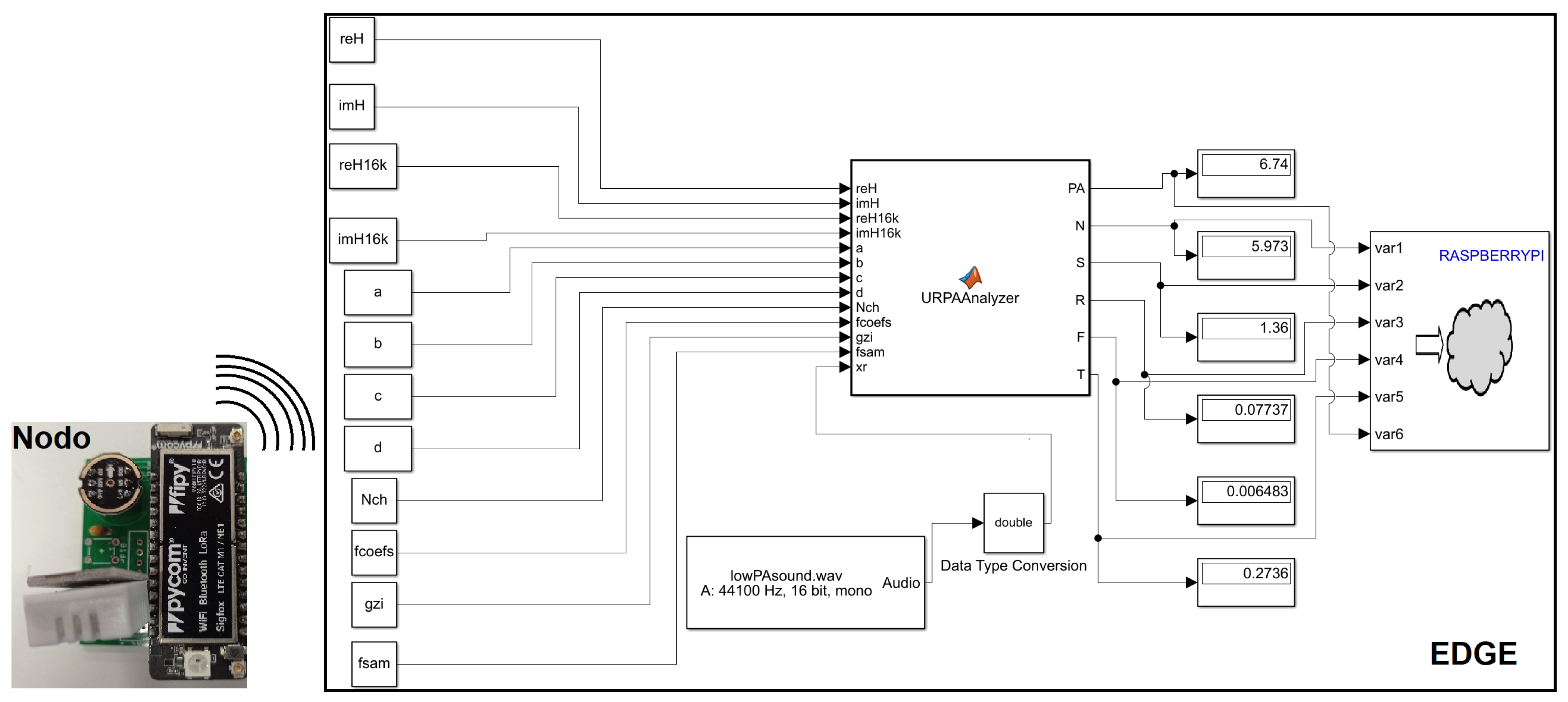
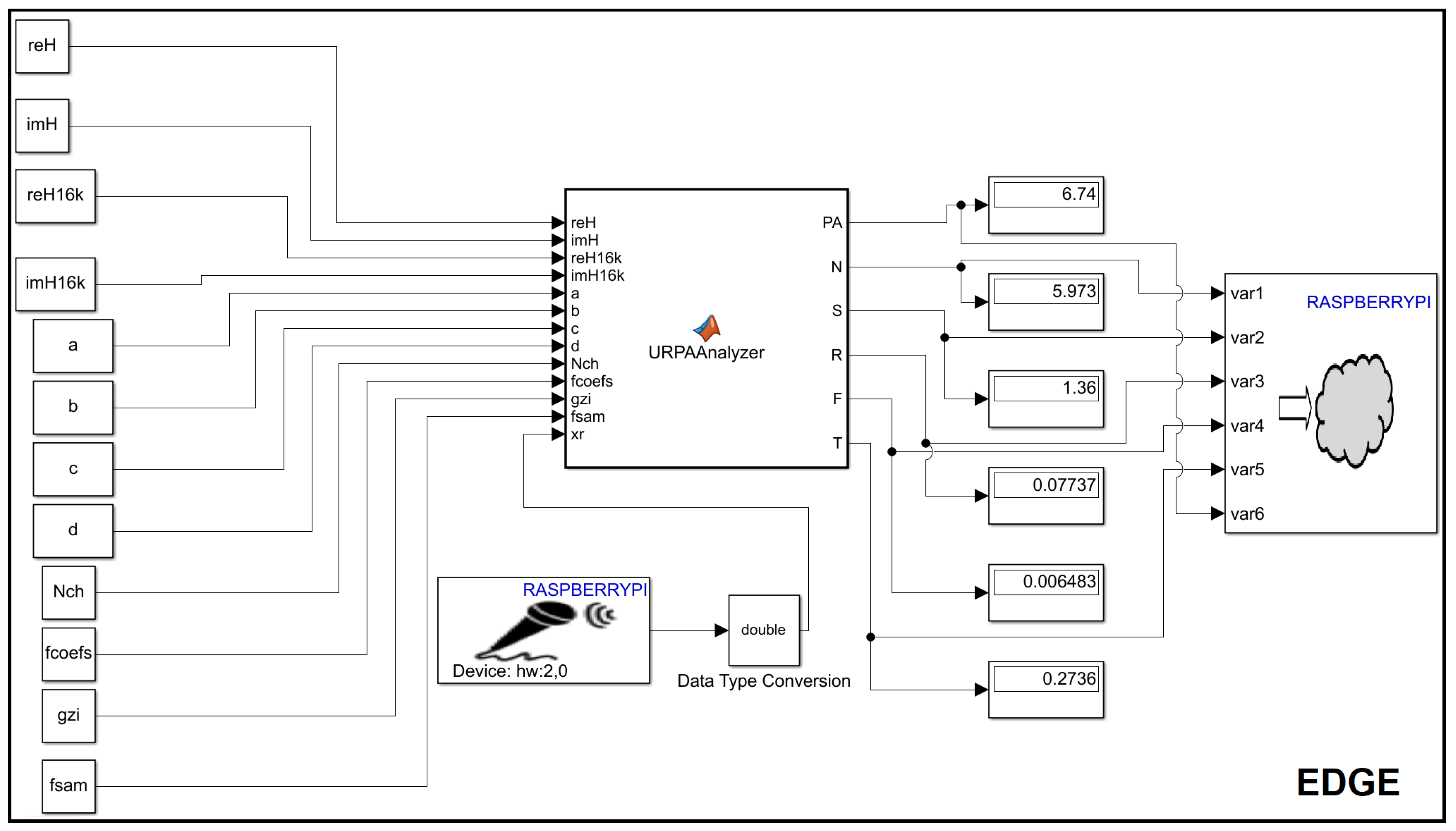
2.3. Implementation of the Architecture of the System

The methodology used in this work to design the system follows a double strategy: (a) acquisition and sample of the sound signal, together with the computation of the psycho-acoustic metrics is performed in the edge node of the network, and (b) acquisition and a sample of the sound signal in an external device, e.g., implementation in a Fipy node [39], and then transmission of the audio file to the edge node through the Message Queuing Telemetry Transport (MQTT) protocol for the computation of the metrics.

The different algorithms of the psycho-acoustic metrics N, S, R, F, and T have been implemented in Matlab [9]. Similarly, these algorithms have been integrated into Simulink models that allow their conversion to C/C++ code using the Matlab “coder” tool and their direct installation in Single-Board Computer (SBC)-type platforms. In our case, it has been integrated into a Raspberry Pi 4B+ with 4GB of RAM (RPi4). This platform acts as the edge node of the system, which allows the calculation of the psycho-acoustic metrics from the recorded audio.

Figure 1 (considering Fipy with a microphone and sending the audio to the edge) and Figure 2 (integrating the microphone in the edge) show the Simulink schematic of the complete algorithm that determines the different psycho-acoustic metrics, as well as the modified psycho-acoustic annoyance [25], taking into account the two strategies explained in this section. Both have been implemented.

In Figure 1, the option with Fipy (MCU+modems) from Pycom, where an ESP32 MCU node with various wireless connectivity options (i.e., Wi-Fi, BLE, Lora, Sigfox, and LTE-M/NB-IoT) connected to an INMP441 MEMS microphone, samples audio, performs windowing and sends the audio to the Rpi4, which allows the calculation of the different metrics, is shown. Figure 2 shows the option in which the RPi4 itself, which acts as an Edge, has a USB microphone connected.

In both options, the output, which is an array with different metrics, is sent to an online Cloud. In this work, the Thingspeak platform [40] is used, with MQTT protocol for data communication, because of its quick integration in Matlab.

2.4. Calibration Procedure

The calibration is carried out using a file with sinusoidal tone at 1kHz in the scheme of Figure 1. The result of the loudness with this file is N 40 sones, measuring a sound pressure level of 40 dB (as is stated in the definition of loudness). Additionally, the other parameters are fixed according to its definition in the Matlab-generated code.

2.5. Experiments to Evaluate the Model

Two different experiments were carried out to evaluate the performance of the implemented model. First, a comparison of both models’ results was made in a laboratory scenario, and second, the sound was acquired by deploying acoustic nodes in a real scenario.

In the first experiment, after the calibration procedure, the psycho-acoustic parameter values of a pneumatic hammer from a digital recording (https://www.youtube.com/watch?v=_MDzFgznDxg&t=34s –pneumatic hammer recording–(accessed on 13 April 2023)) were measured for 17 min. This sound source was rendered using a Behringer MS16 loudspeaker and the sound was captured with the RPi4, sending values in the cloud every 1 s.

In the application of the proposed system to a real scenario, a set of single-board computers (SBC), in particular Raspberry Pi 4B+, was used to deploy a wireless acoustic sensor network across the campus of the Universidad Católica de Murcia (UCAM), located in Murcia, Spain. Figure 3 shows the location of the seven nodes distributed in three different soundscapes, both indoors, a canteen, and a monastery cloister, and outdoors, in a square called pergolas.

Results are presented and discussed in the following Section 3.1 and Section 3.2, respectively.

3. Results and Discussion

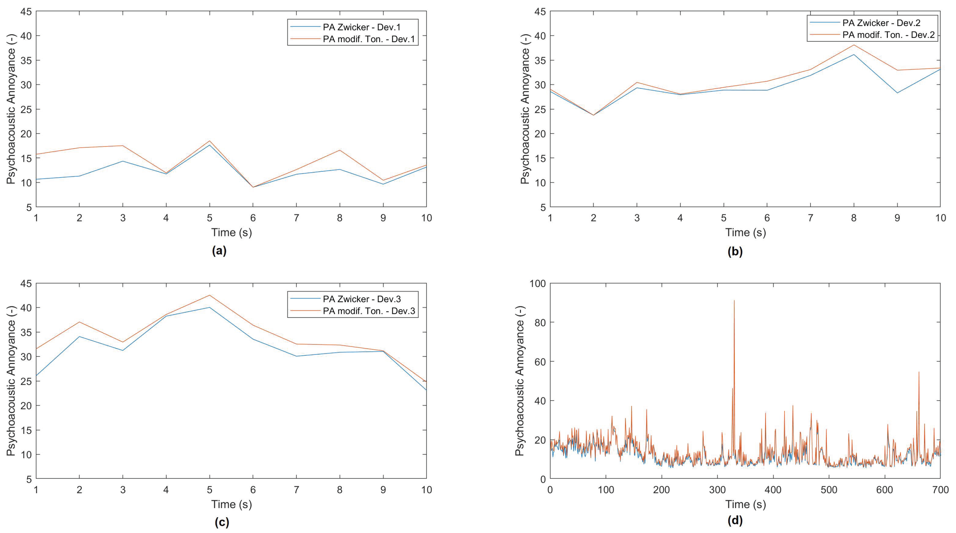
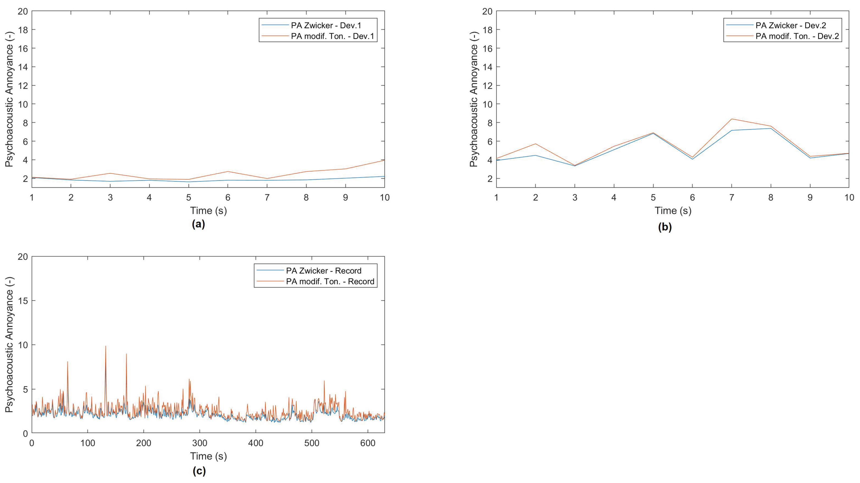
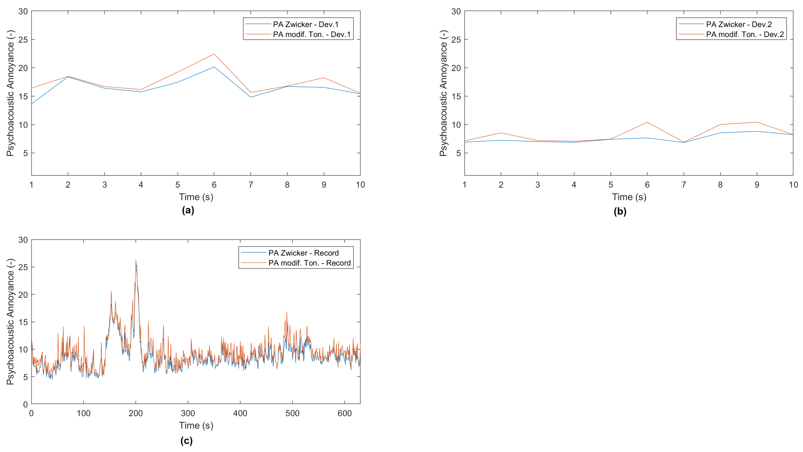
3.1. Application of the System to Compare Models’ Results

The produced PA by the pneumatic hammer sound emission has been calculated using both the basic Zwicker model, Equation (1), and the modified model with tonality, Equation (2a,b). Figure 4 shows the values calculated with these two models (Zwicker’s PA and modified PA with tonality), showing that the appearance of tonal sounds in a noisy environment produces greater subjective annoyance. The calculation of the annoyance model with the tonality was launched, and it can be seen in this figure with increased values. It is also observed that this noise, although annoying at certain levels, is not very tonal, so a large percentage of the measurements of the two models coincide.

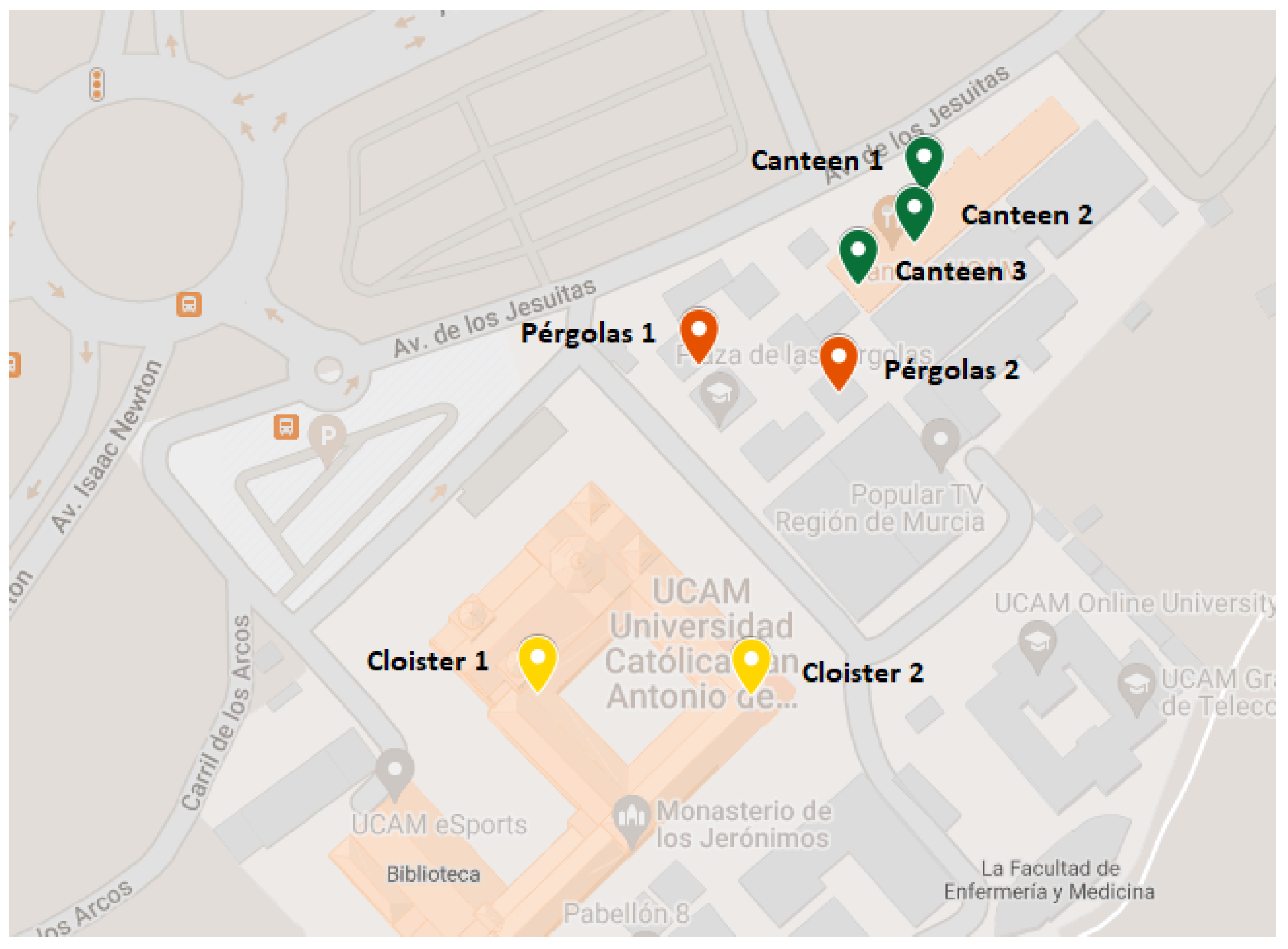
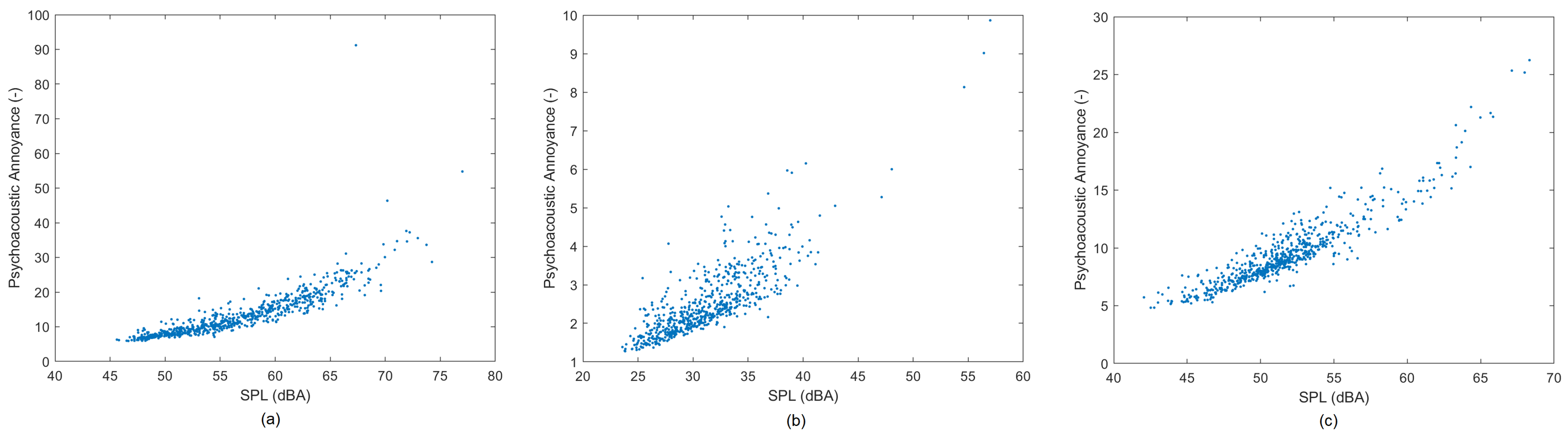
3.2. Application of the System to a Real Scenario: UCAM Campus

Figure 5 shows the results of a 10 s measurement (one shot) in the three devices located at the canteen (Figure 5a–c). Moreover, results from a long recording (700 s) in an intermediate location within the canteen are shown in Figure 5d. This zone is one of the busiest areas of the campus; therefore, it is observed that the psycho-acoustic annoyance is higher at specific moments due to a higher concentration of people.

Additionally, Figure 6 shows the plots of 10 s measurement in two devices located in the cloister of the monastery of the UCAM (Figure 6a,b). The low annoyance is one of the main characteristics in this location, as shown in the long recording (630 s) (Figure 6c).

The third environment, pergolas square, is an outdoor zone that can be both crowded and quiet depending on the time of day since staff and students can use the space during break times. Figure 7 shows the psycho-acoustic annoyance of a 10 s measurement of two deployed devices in this square (Figure 7a,b). At the moment when the measurement was made, the outdoor environment was quite calm, and the nuisance was not too high, as it is shown in the long recording (640 s) (Figure 7c).

Figure 8 shows the relationship between SPL, in dBA, and the psycho-acoustic annoyance in the three locations on the UCAM campus, the canteen (Figure 8a), the cloister (Figure 8b) and the outdoor pergolas (Figure 8c). The three cases show a quasi-linear relationship, as the main contribution is made with the loudness, as shown in [38], although there are slight differences generated by tonality, roughness, and fluctuation strength, as shown in Figure 5, Figure 6 and Figure 7.

3.3. JND in the UCAM Campus

With the values obtained in the error propagation considered in Section 2.2, the application of $\Delta PA$ produces a range of JNDs for Zwicker’s psycho-acoustic annoyance in the canteen of the campus with an average value for $\Delta PA$ of 0.3553 and a variance value of 0.1012, which determines a mean percentage of 4.2% of relative variation for the PA ($\Delta PA/PA$) to have perceptual a change in this environment. In the cloister area of the campus, the mean value for the PA JND is 0.7489 and the variance is 0.0044, which determines a mean percentage of 38.7% of relative variation for the PA ($\Delta PA/PA$) to have perceptual a change in this environment. This value means that silent places can have a higher variation in the perception of annoyance. In the case of the outdoor pergolas, the PA JND has a mean value of 0.5008 and a variation value of 0.0289, which determines a percentage of 6.6% of relative variation for the PA ($\Delta PA/PA$) to have a perceptual change in this environment.

4. Conclusions

This paper presents different implementation options for a modified psycho-acoustic annoyance algorithm and compares it with Zwicker’s psycho-acoustic annoyance, introducing a term that weights the tonality of sounds. These algorithms were implemented in a different Raspberry Pi 4B+ and applied to different locations in the UCAM Campus in Murcia (Spain). According to the authors in [37], the JNDs of PA values computed from sound-quality metrics obtained in these measurements are kept in a range between 4% and 38% depending on the environment. According to our experience in this study, silent places can have a higher variation in the perception of annoyance.

The model exported to an SBC (RPi4B) has been applied to measure noise generated by a recorded pneumatic hammer and different locations on the campus. It has been observed that from the values calculated with the two models, the occurrence of tonal sounds in a noisy environment produces greater subjective annoyance. The MATLAB implementation to integrate into the RPI4B+ with the codegen command has been published in https://github.com/jausegar/urbauramon/tree/master/URPAA_Rasp_simulink (accessed on 20 June 2023).

Both implementations, the one from Figure 1 and the one from Figure 2, showed a good performance in computing all the metrics in real time, but the offloading in the first case allowed a better performance as the computing load in the sampling and windowing was carried out in the external node.

For future work, it is intended to extend this study to a larger number of noisy environments to describe other soundscapes for classification purposes.

References

1. ISO 12913-1:2014; Acoustics—Soundscape—Part 1: Definition and Conceptual Framework. ISO: Geneva, Switzerland, 2014.
2. ISO 12913-2:2018; Acoustics—Soundscape—Part 2: Data Collection and Reporting Requirements. ISO: Geneva, Switzerland, 2018.
3. Dunbavin, P. ISO/TS 12913-2:2018—Soundscape—Part 2: Data collection and reporting requirements—What’s it all about? Acoust. Bull. 2018, 43, 55–57. [Google Scholar]
4. Lopez-Ballester, J.; Pastor-Aparicio, A.; Felici-Castell, S.; Segura-Garcia, J.; Cobos, M. Enabling Real-Time Computation of Psycho-Acoustic Parameters in Acoustic Sensors Using Convolutional Neural Networks. IEEE Sens. J. 2020, 20, 11429–11438. [Google Scholar] [CrossRef]
5. Montoya-Belmonte, J.; Navarro, J.M. Long-Term Temporal Analysis of Psychoacoustic Parameters of the Acoustic Environment in a University Campus Using a Wireless Acoustic Sensor Network. Sustainability 2020, 12, 7406. [Google Scholar] [CrossRef]
6. Castro, F.L.; Brambilla, G.; Iarossi, S.; Fredianelli, L. The LIFE NEREiDE project: Psychoacoustic parameters and annoyance of road traffic noise in an urban area. In Proceedings of the Euronoise Conference (Euronoise 2018), Heraklion, Greece, 27–31 May 2018. [Google Scholar]
7. Yang, X.; Wang, Y.; Zhang, R.; Zhang, Y. Physical and Psychoacoustic Characteristics of Typical Noise on Construction Site: “How Does Noise Impact Construction Workers’ Experience?”. Front. Psychol. 2021, 12, 3143. [Google Scholar] [CrossRef] [PubMed]
8. ISO 532:2017; Acoustics—Methods for Calculating Loudness—Part 1: Zwicker Method; Part 2: Moore-Glasberg Method. ISO: Geneva, Switzerland, 2017.
9. Pastor-Aparicio, A.; Segura-Garcia, J.; Lopez-Ballester, J.; Felici-Castell, S.; García-Pineda, M.; Pérez-Solano, J.J. Psychoacoustic Annoyance Implementation With Wireless Acoustic Sensor Networks for Monitoring in Smart Cities. IEEE Internet Things J. 2020, 7, 128–136. [Google Scholar] [CrossRef]
10. Engel, M.; Fiebig, A.; Pfaffenbach, C.; Fels, J. A Review of the Use of Psychoacoustic Indicators on Soundscape Studies. Curr. Pollut. Rep. 2021, 7, 359–378. [Google Scholar] [CrossRef]
11. Arce, P.; Salvo, D.; Piñero, G.; Gonzalez, A. FIWARE based low-cost wireless acoustic sensor network for monitoring and classification of urban soundscape. Comput. Netw. 2021, 196, 108199. [Google Scholar] [CrossRef]
12. Chen, C.Y. Monitoring time-varying noise levels and perceived noisiness in hospital lobbies. Build. Acoust. 2021, 28, 35–55. [Google Scholar] [CrossRef]
13. Bonet-Solà, D.; Martínez-Suquía, C.; Alsina-Pagès, R.M.; Bergadà, P. The Soundscape of the COVID-19 Lockdown: Barcelona Noise Monitoring Network Case Study. Int. J. Environ. Res. Public Health 2021, 18, 5799. [Google Scholar] [CrossRef]
14. Hong, J.Y.; Jeon, J.Y. Influence of urban contexts on soundscape perceptions: A structural equation modeling approach. Landsc. Urban Plan. 2015, 141, 78–87. [Google Scholar] [CrossRef]
15. Jo, H.I.; Jeon, J.Y. Overall environmental assessment in urban parks: Modelling audio-visual interaction with a structural equation model based on soundscape and landscape indices. Build. Environ. 2021, 204, 108166. [Google Scholar] [CrossRef]
16. Masullo, M.; Toma, R.A.; Maffei, L. Effects of Industrial Noise on Physiological Responses. Acoustics 2022, 4, 733–745. [Google Scholar] [CrossRef]
17. Manohare, M.; Garg, B.; Rajasekar, E.; Parida, M. Evaluation of change in heart rate variability due to different soundscapes. Noise Mapp. 2022, 9, 234–248. [Google Scholar] [CrossRef]
18. Li, Z.; Kang, J. Sensitivity analysis of changes in human physiological indicators observed in soundscapes. Landsc. Urban Plan. 2019, 190, 103593. [Google Scholar] [CrossRef]
19. Fastl, H.; Zwicker, E. Psychoacoustics: Facts and Models; Springer Series in Information Sciences; Springer: Berlin/Heidelberg, Germany, 2007. [Google Scholar]
20. Moore, B.C.J.; Glasberg, B.R.; Baer, T. A Model for the Prediction of Thresholds, Loudness, and Partial Loudness. J. Audio Eng. Soc. 1997, 45, 224–240. [Google Scholar]
21. Caniato, M.; Zaniboni, L.; Marzi, A.; Gasparella, A. Evaluation of the main sensitivity drivers in relation to indoor comfort for individuals with autism spectrum disorder. Part 1: Investigation methodology and general results. Energy Rep. 2022, 8, 1907–1920. [Google Scholar] [CrossRef]
22. Caniato, M.; Zaniboni, L.; Marzi, A.; Gasparella, A. Evaluation of the main sensitivity drivers in relation to indoor comfort for individuals with autism spectrum disorder. Part 2: Influence of age, co-morbidities, gender and type of respondent on the stress caused by specific environmental stimuli. Energy Rep. 2022, 8, 2989–3001. [Google Scholar] [CrossRef]
23. Bettarello, F.; Caniato, M.; Scavuzzo, G.; Gasparella, A. Indoor Acoustic Requirements for Autism-Friendly Spaces. Appl. Sci. 2021, 11, 3942. [Google Scholar] [CrossRef]
24. Yonemura, M.; Lee, H.; Sakamoto, S. Subjective Evaluation on the Annoyance of Environmental Noise Containing Low-Frequency Tonal Components. Int. J. Environ. Res. Public Health 2021, 18, 7127. [Google Scholar] [CrossRef]
25. Di, G.Q.; Chen, X.W.; Song, K.; Zhou, B.; Pei, C.M. Improvement of Zwicker’s psychoacoustic annoyance model aiming at tonal noises. Appl. Acoust. 2016, 105, 164–170. [Google Scholar] [CrossRef]
26. Shrestha, M.; Zhong, Z. Sound Quality User-Defined Cursor Reading Control-Tonality Metric. Master’s Thesis, IMM (Informatics and Mathematical Modelling), DTU (Technical University of Denmark), Brüel & Kjær, Naerum, Denmark, 2003. [Google Scholar]
27. Estreder, J.; Piñero, G.; de Diego, M.; Rämö, J.; Välimäki, V. Improved Aures tonality metric for complex sounds. Appl. Acoust. 2023, 204, 109238. [Google Scholar] [CrossRef]
28. DIN45631/A1:2010; Calculation of Loudness Level and Loudness from the Sound Spectrum-Zwicker Method-Amendment 1: Calculation of the Loudness of Time-Variant Sound. Deutsches Institut Fur Normung E.V. (German National Standard), Beuth Verlag GmbH: Berlin, Germany, 2010.
29. DIN45692/A1:2009; Measurement Technique for the Simulation of the Auditory Sensation of Sharpness. Deutsches Institut Fur Normung E.V. (German National Standard), Beuth Verlag GmbH: Berlin, Germany, 2009.
30. Jourdes, V. Estimation of Perceived Roughness. Master’s Thesis, Technische Universiteit Eindhoven, Eindhoven, The Netherland, 2004. [Google Scholar]
31. Daniel, P.; Weber, R. Psychoacustical Roughness: Implementation of an Optimized Model. Acustica 1997, 83, 113–123. [Google Scholar]
32. Aures, W. Procedure for Calculating the Sensory Euphony of Arbitrary Sound Signals. Acustica 1985, 59, 130–141. [Google Scholar]
33. Terhardt, E.; Stoll, G.; Seewann, M. Algorithm for extraction of pitch and pitch salience from complex tonal signals. J. Acoust. Soc. Am. 1982, 71, 679–688. [Google Scholar] [CrossRef]
34. Stiegler, L.N.; Davis, R. Understanding Sound Sensitivity in Individuals with Autism Spectrum Disorders. Focus Autism Other Dev. Disabil. 2010, 25, 67–75. [Google Scholar] [CrossRef]
35. Lucker, J.R. Auditory Hypersensitivity in Children with Autism Spectrum Disorders. Focus Autism Other Dev. Disabil. 2013, 28, 184–191. [Google Scholar] [CrossRef]
36. Just Noticeable Difference. Available online: https://en.wikipedia.org/wiki/Just-noticeable_difference (accessed on 18 April 2023).
37. You, J.; Jeon, J.Y. Just noticeable differences in sound quality metrics for refrigerator noise. Noise Control Eng. J. 2008, 56, 414. [Google Scholar] [CrossRef]
38. Segura-Garcia, J.; Felici-Castell, S.; Perez-Solano, J.J.; Cobos-Serrano, M.; Navarro, J.M. Low-Cost Alternatives for Urban Noise Nuisance Monitoring Using Wireless Sensor Networks. IEEE Sens. J. 2015, 15, 836–844. [Google Scholar] [CrossRef]
39. Pycom.io. Fipy, Five Network Development Board for IoT. 2022. Available online: https://pycom.io/product/fipy/ (accessed on 28 December 2022).
40. ThingSpeak. IoT Analytics-ThingSpeak Internet of Things. 2023. Available online: https://thingspeak.com/ (accessed on 13 April 2023).
Figure 1. Simulink model for the determination of psycho-acoustic annoyance from an audio file in the Edge. Sampling is performed by the Fipy node.
Sustainability 15 10016 g001
Figure 2. Simulink model for the determination of psycho-acoustic annoyance from a microphone connected to the Edge. Sampling is performed by the Edge itself.
Sustainability 15 10016 g002
Figure 3. Location of the nodes for the measurement campaign in UCAM Campus—Murcia.
Sustainability 15 10016 g003
Figure 4. Representation of psycho-acoustic annoyance (PA) measurements with the Zwicker model (blue) and with the modified model (orange) of a pneumatic hammer.
Sustainability 15 10016 g004
Figure 5. Recording of psycho-acoustic annoyance (PA) measurements with the Zwicker model (blue) and with the modified model (orange) in the canteen in UCAM Campus-Murcia. Subfigures (ac) correspond to 10 s record with each device in the canteen. Subfigure (d) corresponds to a long recording (with a Zoom recorder) in the canteen.
Sustainability 15 10016 g005
Figure 6. Recording of psycho-acoustic annoyance (PA) measurements with the Zwicker model (blue) and with the modified model (orange) in the cloister in UCAM Campus-Murcia. Subfigures (a,b) correspond to 10 s record with each device in the cloister area. Subfigure (c) corresponds to a long recording (with a Zoom recorder) in the cloister area.
Sustainability 15 10016 g006
Figure 7. Recording of psycho-acoustic (PA) annoyance measurements with the Zwicker model (blue) and with the modified model (orange) in the outdoor pergola in UCAM Campus-Murcia. Subfigures (a,b) correspond to 10 s record with each device in the pergolas area. Subfigure (c) corresponds to a long recording (with a Zoom recorder) in the pergolas area.
Sustainability 15 10016 g007
Figure 8. Graphics of the relationship of Sound Pressure Level versus psycho-acoustic annoyance. Subfigure (a) corresponds to the canteen area, (b) to the cloister area and (c) to the outdoor pergolas area.
Sustainability 15 10016 g008
Disclaimer/Publisher’s Note: The statements, opinions and data contained in all publications are solely those of the individual author(s) and contributor(s) and not of MDPI and/or the editor(s). MDPI and/or the editor(s) disclaim responsibility for any injury to people or property resulting from any ideas, methods, instructions or products referred to in the content.