Prediction of Daily Temperature Based on the Robust Machine Learning Algorithms

Abstract

Temperature climate is an essential component of weather forecasting and is vital in predicting future weather patterns. Accurate temperature predictions can assist individuals and organizations in preparing for potential weather-related events such as heat waves or cold snaps. However, achieving precise temperature predictions necessitates thoroughly comprehending the underlying factors influencing climate patterns. The study utilized two models, LSTM and DLSTM, to forecast daily air temperature using 1097 data points gathered from central and southern regions of Tabriz city of Iran in Asia from 2017 to 2019. The results indicated that the proposed model had a high accuracy rate for predicting daily air temperature for test data, with RMSE_DLSTM = 0.08 °C and R-Square_DLSTM = 0.99. The DLSTM algorithm is known for its high speed, accuracy, time series prediction, noise reduction capabilities for data, the large volume of data processing, and improved performance of predicted data. In summary, while both LSTM and DLSTM are used for predicting data points, DLSTM is a more advanced version that includes multiple layers of memory cells and is better suited for handling complex sequences of events.

1. Introduction

Weather research is of global interest to scientific centers because of its essential role in human life, agriculture, and industry. The weather directly impacts the economy, human health, food security, and energy consumption [1]; the likelihood of disasters, such as severe droughts and urban floods, increases with weather change [2]. Additionally, when the temperature of the weather changes, the water quality of rivers worldwide is affected by this change [3]. These issues made the need for a new approach, including an important matter such as weather forecasting, to be felt more than ever. Forecasting temperature is crucial and helpful in understanding climate factors. By predicting weather conditions, it is possible to minimize the negative impact of weather and enhance various social benefits such as safeguarding lives and property, promoting public health and safety, improving economic prosperity, and enhancing the overall quality of life [4,5]. Improved weather prediction can have significant social, health, environmental, and economic benefits, including enhanced disaster preparedness, increased agricultural productivity, and reduced energy consumption [6]. In addition, air temperature fluctuations can have significant health implications, including respiratory problems (changes in air temperature can worsen respiratory conditions such as asthma and chronic obstructive pulmonary disease (COPD). Cold air can also trigger bronchospasms in people with asthma) [7], cardiovascular problems (extreme temperatures can put a strain on the heart and increase the risk of heart attacks and other cardiovascular problems) [8], and mental health issues (extreme temperatures can also affect mental health, causing anxiety, depression, and other mood disorders) [9]. Improved prediction models can provide short-term benefits, such as better agricultural planning, and long-term benefits, such as improved infrastructure planning for vulnerable populations living in regions with high climate variability [10].

Numerical weather prediction (NWP) is a commonly used temperature forecasting method involving simulating the atmosphere [11]. By the authors [12] conducted a study using models, satellite remote sensing, and reanalysis products to illustrate droughts in South Asia from 1982 to 2019 using a standardized index/anomaly approach. They found that MERRA-2, CPC, FLDAS, GPCC, and CHIRPS were constant over the entire region, while GLDAS and ERA5 were poor compared to other soil moisture products. TWS products such as MERRA-2 TWS and GRACE TWS showed irregular drought patterns, and VCI was less responsive in certain regions. The results of this investigation have facilitated the forecasting of drought occurrences and the surveillance of agricultural activities [13].

The study by the authors [14] uses global climate models and population projections to assess the future changes in high-temperature extremes and exposure to the population in Africa by the mid-21st century. The intensity of high-temperature extremes is expected to increase between 0.25 to 1.8 °C and 0.6 to 4 °C under two different scenarios, with Southern Africa projected to warm faster than other regions. By the mid-21st century, continental population exposure is expected to increase by ~25%, with the highest increase in exposure expected in most parts of West Africa, followed by East Africa [14]. The authors [15] investigated the projected heat stress and associated socioeconomic exposure across South Asia using climate models, population, and GDP projections. They found that the region has the potential for widespread changes to wet bulb globe temperature (WBGT), which can exceed human tolerance by the mid-21st century. The exposure of the population and GDP is expected to significantly increase during mid-term and long-term periods under different scenarios, with the highest upsurge in exposure anticipated for southern Pakistan and southwestern India [15]. The authors [15] studied the projected heat stress and associated socioeconomic exposure across South Asia and its subregions using 23 global climate models. They found that the region has the potential for widespread changes in wet bulb globe temperature (WBGT), which can exceed the theoretical limits of human tolerance by the mid-21st century. They also found that the GDPt causes changes in climate change [13].

In the last few years, many researchers have been able to predict essential parameters for different industries and areas using artificial intelligence [16,17,18,19]. Some researchers who have been able to predict the amount of resin by using artificial intelligence algorithms include the following:

The authors [20] utilized two machine learning models, support vector regression (SVR) and extreme gradient boosting (XGBoost), to forecast surface air temperature (SAT) during winter in North America. The authors compared the performance of these models with the linear regression (LR) model and found that both SVR and XGBoost models outperformed the LR model [20]. The authors [21] employed two models, neuro fuzzy inference system (AN-FIS) and support vector regression (SVR), to predict rainfall using relative humidity, wind, and temperature data obtained from the Meteorological Maritime Station, Meteorological Climatological and Geophysics Agency Perak II Surabaya. The results revealed that the SVR method performed better with an MSE error value of 0.0928 [21]. Hanoon’s study in 2021 used gradient boosting tree (G.B.T.), random forest (R.F.), linear regression (LR), and different artificial neural network architectures such as multi-layered perceptron and radial basis function for forecasting air temperature (T) and relative humidity (Rh). The study concluded that MLP-NN had the best performance for predicting temperature and humidity compared to other models [22]. Gad and Doreswamy’s research in 2022 compared various methods such as linear regression, support vector machine, decision tree, linear discriminant analysis, Gaussian NB, random forest, k-nearest neighbors, AdaBoost, extreme gradient boosting ensemble method, artificial neural networks such as multi-layer perceptron MLP and deep learning for predicting weather conditions. The experimental results demonstrated that the decision tree CART, XGBoost, and AdaBoost models exhibited better classification accuracy when compared with other methods. For regression tasks, the linear regression method performed better in terms of R² metric [23]. According to [24], various methods, including autoregressive integrated moving average (ARIMA), Error–Trend–Seasonality (ETS), exponential smoothing state space model with Box–Cox transformation (TBATS), dynamic harmonic regression (DHR), neural network autoregression (NNAR) method, support vector regression (SVR), and long short-term memory (LSTM) were compared to forecast future weather patterns in central Croatia. The study revealed that SVR is the most effective method, while DHR and NNAR methods outperformed other evaluated methods regarding forecasting accuracy. The DHR method was more suitable for predicting temperature and air pressure, whereas the NNAR method was better for predicting precipitation [24].

The current study has been presented to predict the critical parameter of climate fluctuations and changes, daily air temperature. This article utilizes 1097 data points gathered from the central and southern regions of Tabriz city of Iran in Asia from 2017 to 2019. The data was obtained from the world weather website. The input data related to the prediction of this critical parameter includes the time series Tt-3, Tt-2, and Tt-1. The developed LSTM deep learning algorithm has been used to predict this critical parameter. The use of this algorithm distinguishes this work from other researchers’ articles. The DLSTM algorithm has several advantages over other recurrent neural networks. Firstly, it has multiple memory cells that enable it to store information longer, making it ideal for long-term memory tasks. Secondly, it can make accurate predictions even when dealing with complex and large datasets by learning patterns and relationships in the data. Thirdly, it is robust to noise and missing data, allowing it to handle missing values by interpolating them based on the available data. Fourthly, it allows for parallel processing, making it faster than other recurrent neural networks.

Additionally, the deep LSTM algorithm is flexible and can be used in various applications such as speech recognition, image captioning, natural language processing, and more. It also has mechanisms that reduce the vanishing gradient problem during backpropagation, making it easier to train deep networks. Lastly, the DLSTM algorithm can extract features from raw data without requiring manual feature engineering, which saves time and effort in the development process.

2. Materials and Methods

2.1. Proposed Models Using a Deep Learning Approach

To accurately predict the proposed model, the time series dataset has been given to the network in a sliding manner [25]. In the machine learning technique, the supervised learning method is usually used, where there are input variables (x) and an output variable (y), an algorithm is used to learn the mapping function from input to output, and its goal is to perform correctly and accurately [26]. The mapping is accurate so that as long as there is new input data (x), the output variables (y) are predicted for that data. In this method, the algorithm repeatedly makes predictions related to the training data., corrects them with updates, and stops learning when the algorithm achieves an acceptable level of performance [27]. Therefore, previous observations (for example, t-1) are used as input variables to predict the desired time step (t) in time series predictions. In this article, the observations are named Var, the time step of the input observations is t-1, and the output time step is t, among the characteristics that influence forecasting [28]. As seen in Figure 1, the data from the beginning to the end includes the influential features, and the last data is related to the patient’s blood sugar level at a time interval of 5 min. In the following, the internal structure of the LSTM cell and details are discussed first, and then two deep neural network models are examined in detail.

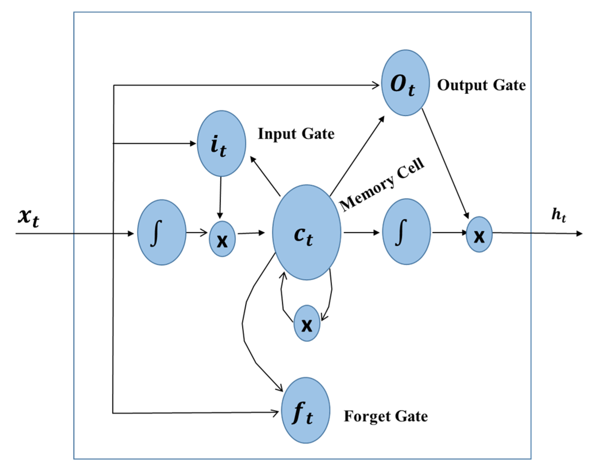
2.2. LSTM Neural Network

Each LSTM cell can easily remember a specific feature in the input stream if necessary for subsequent long-time steps [29]. Therefore, this section discusses the LSTM cell’s internal structure and details [30]. This cell has three gates to control the data flow [31]. These gates include the forgetting gate (ft), update gate (input gate) (it), and output gate (not), and the memory cell is also shown as (ct) Figure 2.

The input data of the LSTM cell is a separate vector of input data xt and new data from ht-1 of the previous cell [32]. The oblivion gate controls the flow of information in the last time step [33]. This gate specifies the problem of using/not using the memory information from the previous time step and the amount of input data from the last time step. It is calculated using the following equation (Equation (1)) [34].

$$f_t=\sigma \left(W_{xf}x+W_{xf}{h}_{t-1}+b_f\right)$$

(1)

The update gate ($i_t$) controls the flow of new information. This gate specifies the use/non-use of further details in the current time step and its amount [35]. This gate, also known as the entrance gate, is calculated as follows (Equation (2)).

$$i_t=\sigma \left(W_{xi}+W_{hi}{h}_{t-1}+b_i\right)$$

(2)

A new vector can be added to the previous memory to update information. For this purpose, Equation (3) is used, and the memory is updated according to Equation (4).

$$c_t^{\prime }=tanh\left(W_{hc}{h}_{t-1}+W_{xc}{x}_t+b_c\right)$$

(3)

$$c_t=f_i{c}_{t-1}+i_t{c}_t^{\prime }$$

(4)

Finally, to specify the content used in the output (h_t), the output gate (o_t) is used in Equations (5) and (6).

$$o_t=\sigma \left(W_{oc}{c}_t+W_{oh}{h}_{t-1}+b_0\right)$$

(5)

$$h_t=o_t\sigma \left(c_t\right)$$

(6)

An LSTM neural network consists of several LSTM cells, receives different input (x_t) in each time step, can produce output (o_t) in each time step, and also has a memory state (h_t) that contains the information [36]. It stores what has happened in the network up to time t.

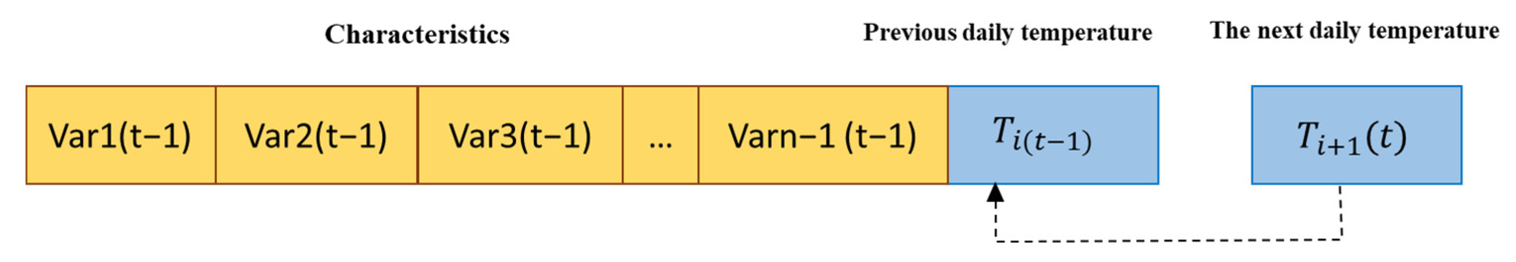
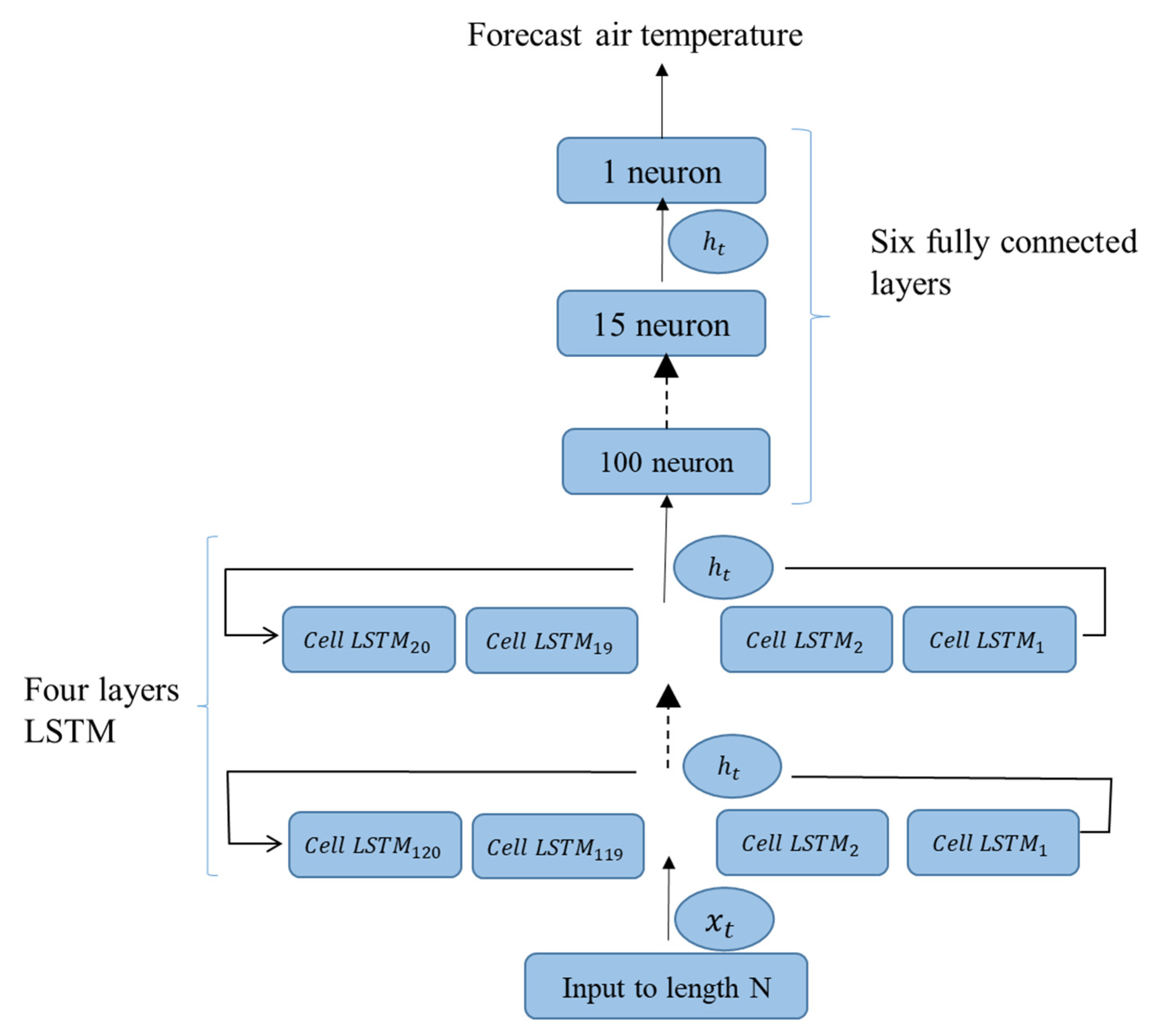
2.3. The Structure of the Neural Network of the First Model

The architecture of the first proposed model is shown in Figure 3, which is designed based on LSTM neural network and feedforward. After several trial-and-error approaches according to the dataset’s size, the first proposed model includes four LSTM and six fully connected layers [37]. First, data is entered into LSTM layers; the first to fourth layers contain 120, 60, 50, and 30 LSTM cells, respectively, and then six completely connected layers are considered. The number of cells of the LSTM layer and the neurons of the fully connected layer is a meta-parameter whose appropriate value can be obtained by trial and error. Therefore, fully connected layers include 100, 85, 60, 30, 15, and 1 neuron, respectively.

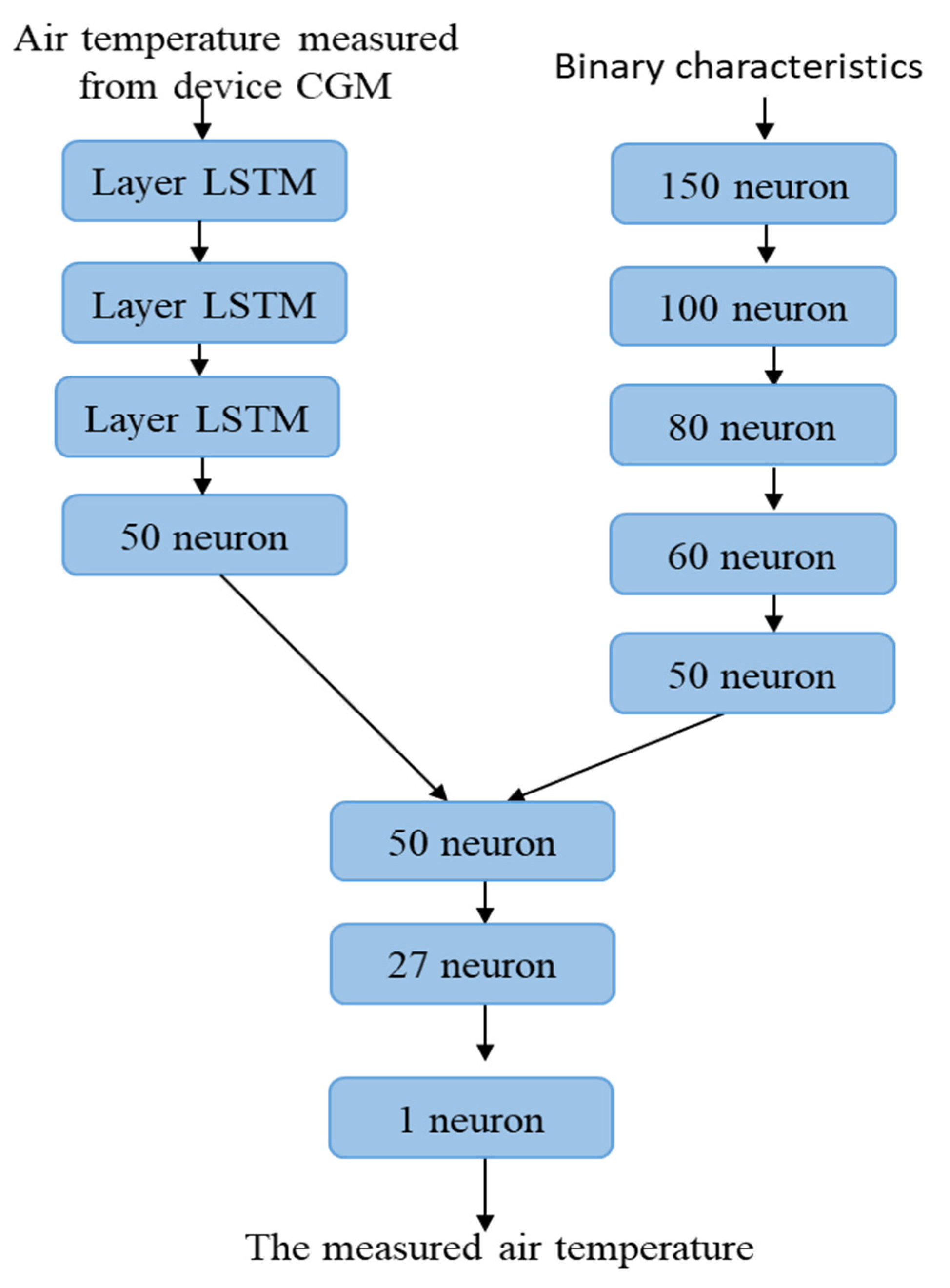
2.4. Examining the Structure of the Neural Network of the Second Model

A view of the architecture of the second model is shown in Figure 4, which is designed based on LSTM neural network and feedforward. It can be seen that the measured air temperature is given as input to the LSTM neural network section [38]. All 27 binary characteristics affecting the air temperature are given as input to the feedforward neural network, and the output of these two networks is entered as input to another feedforward network. This model consists of three separate parts. The part of the proposed model whose input is the air temperature of the patients consists of four layers; the first three layers contain 128, 100, and 60 LSTM cells, respectively, and the last layer contains 50 neutrons.

The other part of the network, whose input is binary characteristics, consists of five fully connected layers that contain 150, 100, 80, 60, and 50 neurons, respectively. The output of these two parts is entered as input to the third part consisting of three wholly connected layers, which include 50, 27, and 1 neuron, respectively.

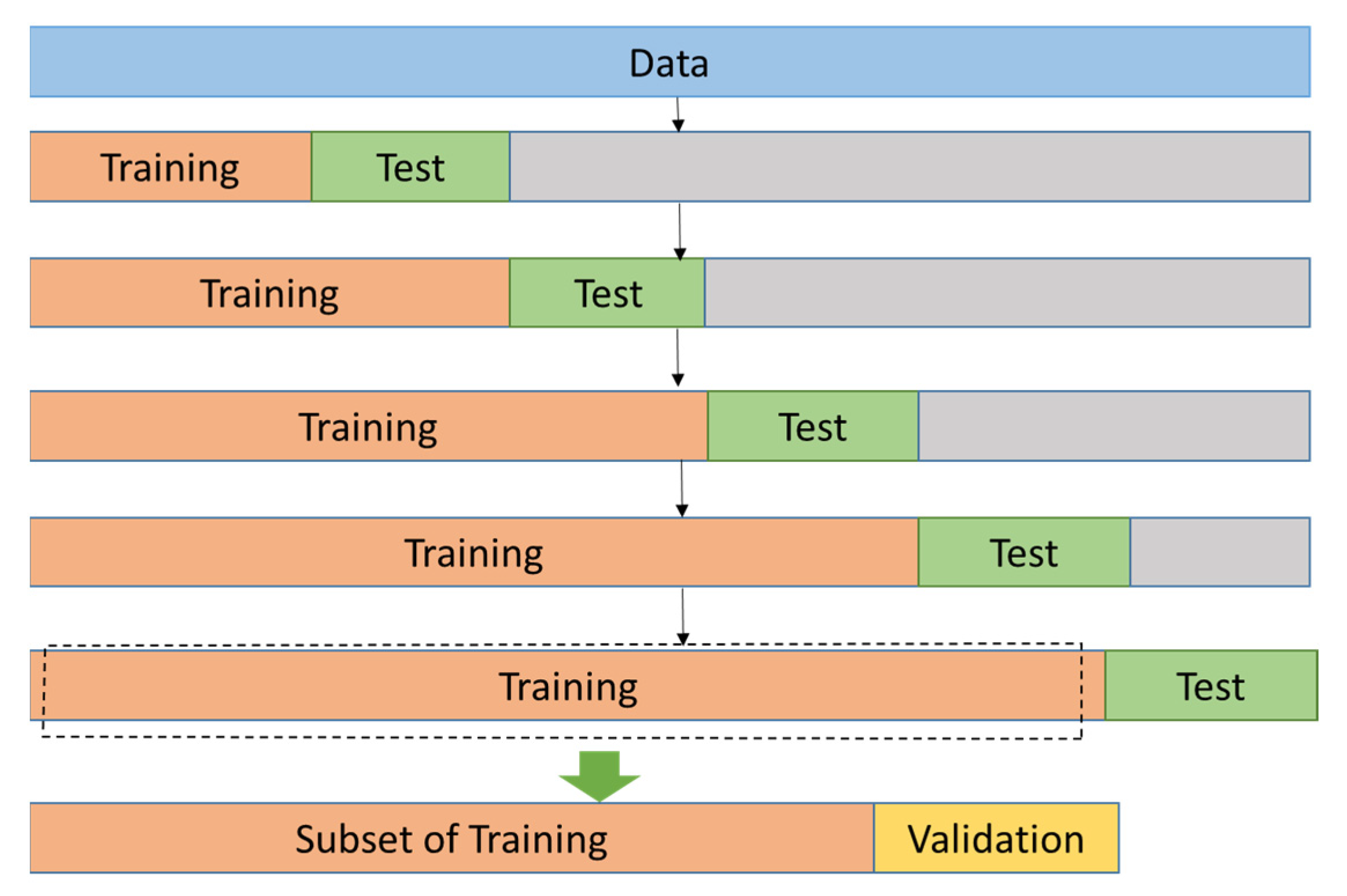
2.5. Neural Network Training of Proposed Models

Based on the investigations carried out in the research conducted in the field of time series prediction using machine learning algorithms, the dataset is divided into two categories, the training and test set, and the set of training has been used to train algorithms [39]. Additionally, the training data is divided into two categories, training and validation, which have been used to evaluate the amount of training obtained from the dataset [40]. Therefore, to accurately assess and reach relevant results, these proposed models have used the k-fold method (an example of cross-validation) [41,42]. However, it is possible to use in time series due to time dependencies and arbitrary test set selection. There is no traditional cross-validation [43]. Therefore, the steps of the validation method used in the time series are as follows.

In the first step, the whole data is divided into several parts. Usually, the default value of this division in conventional implementations is equal to three. In this article, after several testing times, the value of five is considered for data division. As a result, the data is divided into five parts, and one part is selected in each step. In the second stage, the selected part of five parts is divided into training, and test sets and validation are done. In the third stage, another part of the five parts was selected, the domain validated in the second stage was added to this part, and the training and test set was specified and validated. Figure 5 shows that this process continues until all five elements are evaluated. Additionally, the training data has been divided into two parts for accurate evaluation and to achieve satisfactory results: training data and validation data. Approximately 20% of the training data was validated in each step. For example, in the fifth stage of cross-validation, the number of data samples in the training, validation, and test sets is 45,470, 11,370, and 24,360, respectively.

2.6. Meta Parameters

One critical step to achieving the expected results is the right choice of meta-parameters [44]. The selection and quantification of these meta-parameters are usually made experimentally; therefore, most of the parameters in these models are set by trial and error [45].

The MSE cost function is used in the network training process. The MSE function is a statistical tool to find the accuracy of the prediction made in the modeling, which calculates the mean square of the distance between the predicted and the actual value [46].

In deep learning networks, parameters are updated using gradient descent to minimize the value of the cost function. The optimization algorithm based on the cost function and the data determines the direction in which the network weights should be updated so that the network reaches the optimal state [47]. Adam’s optimizer function is used in these models. The learning rate η represents the speed of updating the weights, which can have a constant value or change adaptively. The Adam function is a method to adjust the learning rate in the training process according to the parameters. In the models, the learning rate parameter in the Adam optimizer is equal to 0.001. The parameters with a higher occurrence rate have fewer changes, and the ones that occur less often have more updates [47].

Usually, for training neural networks, the data is grouped to be more accessible regarding speed and parallelism. The batch size meta parameter indicates the number of samples from the training dataset used in the error gradient estimation and the number of data samples based on the updated network weights. The batch size parameter is an important parameter affecting the learning algorithm’s dynamics. Choosing the wrong value for this meta-parameter causes poor network performance [48]. Using the trial-and-error approach, the size of this data category is considered equal to 72 in the models. Additionally, this model uses the accuracy evaluation criterion, which expresses the ratio of correctly predicted observations to all data. Among other meta-parameters, we can mention the number of neurons in each layer, discussed in the neural network structure review section. The final settings of the meta-parameters of the proposed models are presented in

Table 1. Free parameter settings in the network of the first and second models.

Meta Parameter	Settings
Activation function	SELU, ReLU
Cost dependent	MSE
Batch size	72
Learning rate	0/001
Optimizer	Adam
Maximum number of iterations	100
The number of network layers	The first model:10 The second model:12

.

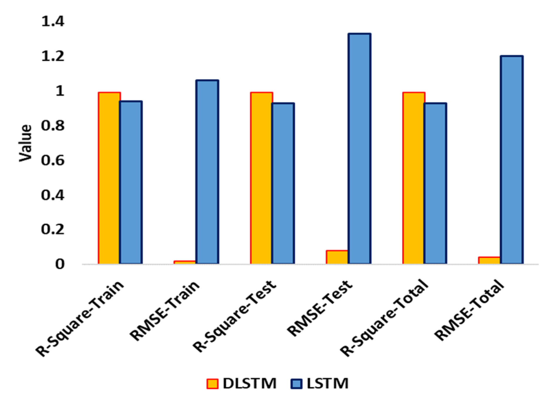
2.7. Error Parameters

One of the essential parameters for determining the statistical error for predicting statistical data and determining the performance accuracy of algorithms is the use of mean square (MSE), standard deviation (SD), absolute average relative (AARE), square error (RMSE) and R-square, average relative error (ARE), parameters.

$$ARE=\frac{{{\sum }_{i=1}^n(\frac{T_M - T_P}{T_M})}_i}{n}$$

(7)

$$AARE=\frac{{\sum }_{i=1}^n\left|{(\frac{T_M - T_P}{T_M})}_i\right|}{n}$$

(8)

$$SD=\sqrt{\frac{{\sum }_{i=1}^n{(({\frac{1}{n}{\sum }_{i=1}^n\left({T_M}_i - {T_P}_i\right)}_i)-({\frac{1}{n}{\sum }_{i=1}^n\left({T_M}_i - {T_P}_i\right)}_{mean}))}^2}{n-1}}$$

(9)

$$MSE=\frac{1}{n}\sum _{i=1}^n{\left({T_M}_i - {T_P}_i\right)}^2$$

(10)

$$RMSE=\sqrt{MSE}=\frac{1}{n}\sum _{i=1}^n{\left({T_M}_i-{T_P}_i\right)}^2$$

(11)

$$\mathrm{R}-\mathrm{s}\mathrm{q}\mathrm{u}\mathrm{a}\mathrm{r}\mathrm{e}=1-\frac{{\sum }_{i=1}^N{({T_P}_i-{T_M}_i)}^2}{{\sum }_{i=1}^N{({T_P}_i-\frac{{\sum }_{i=1}^n{T_M}_i}{n})}^2}$$

(12)

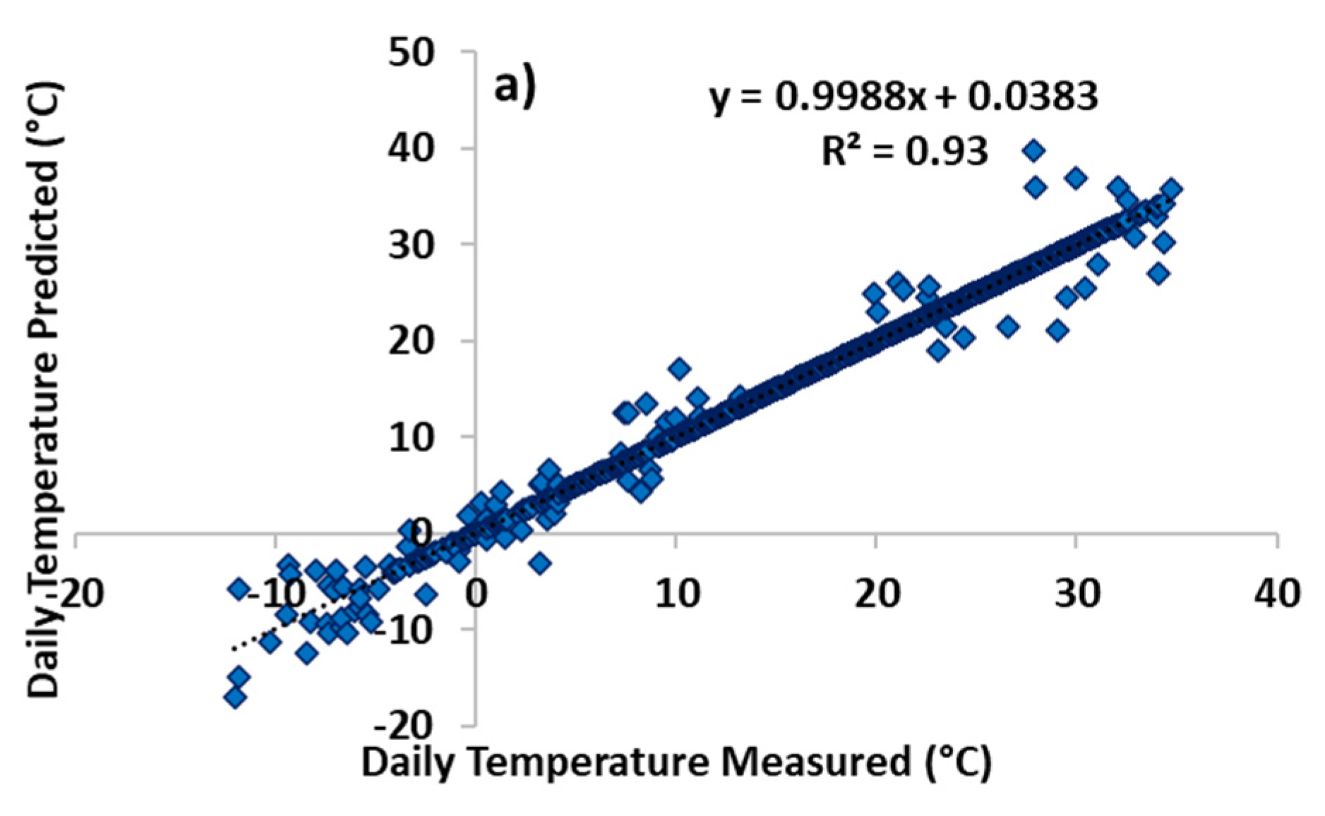
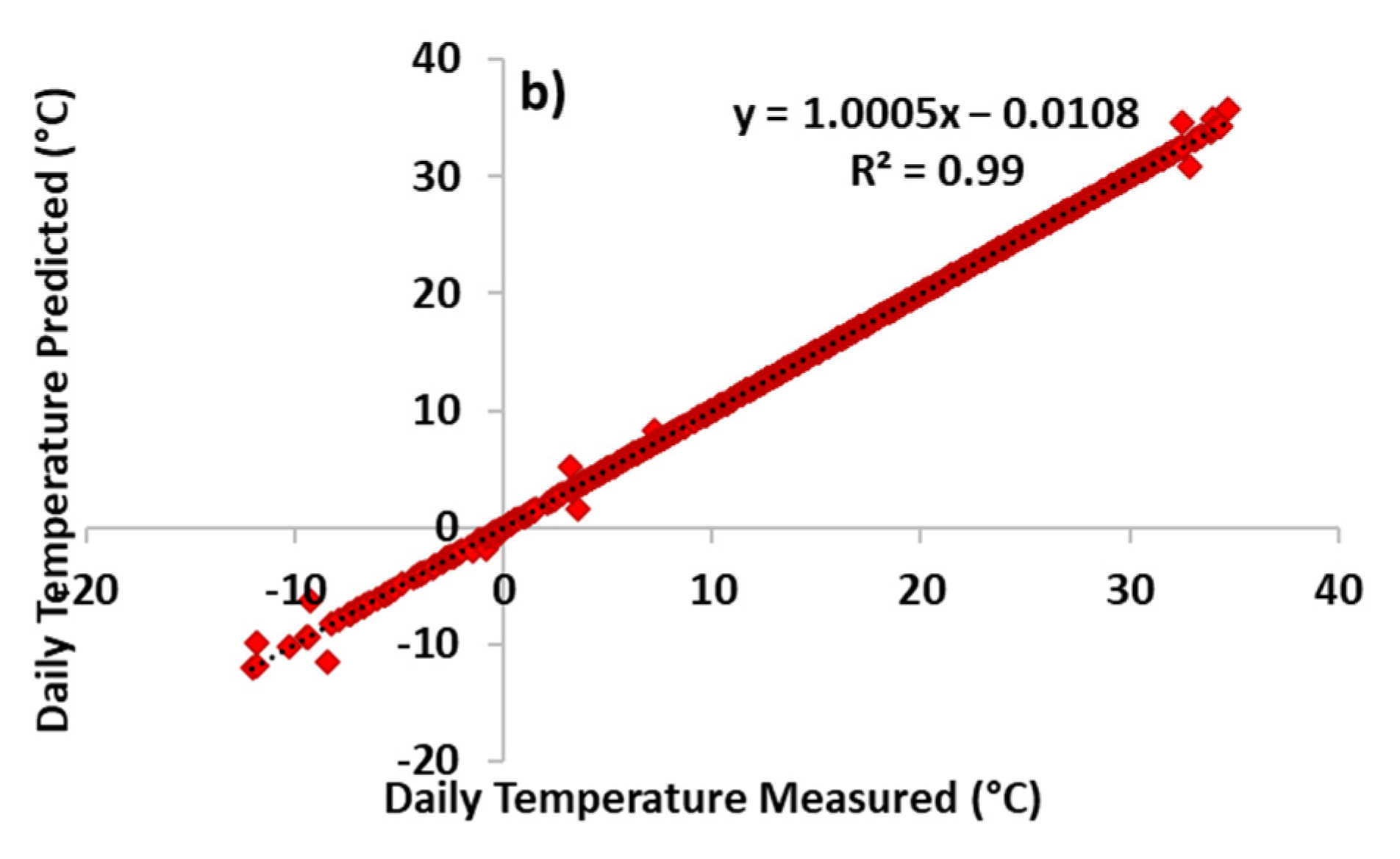
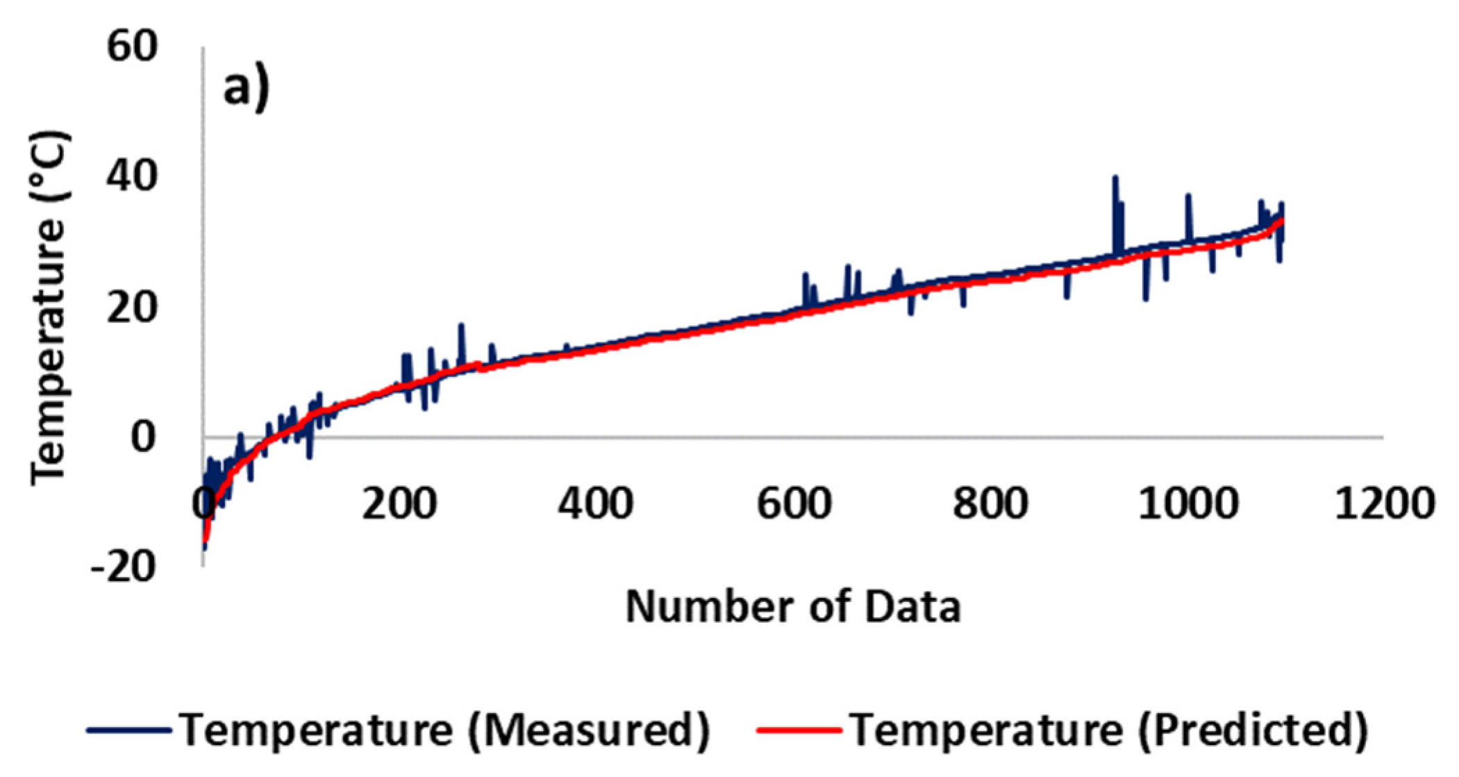
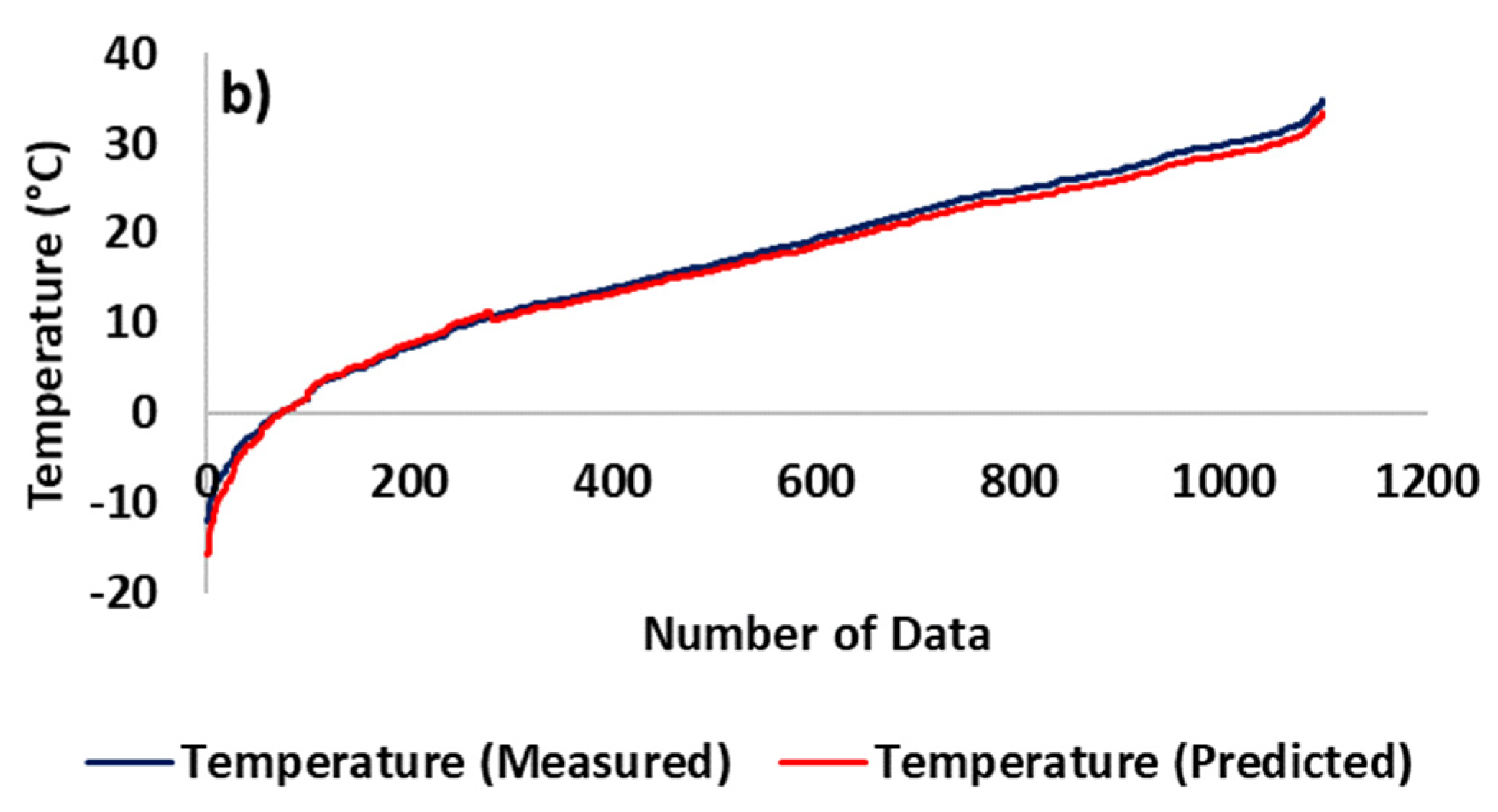
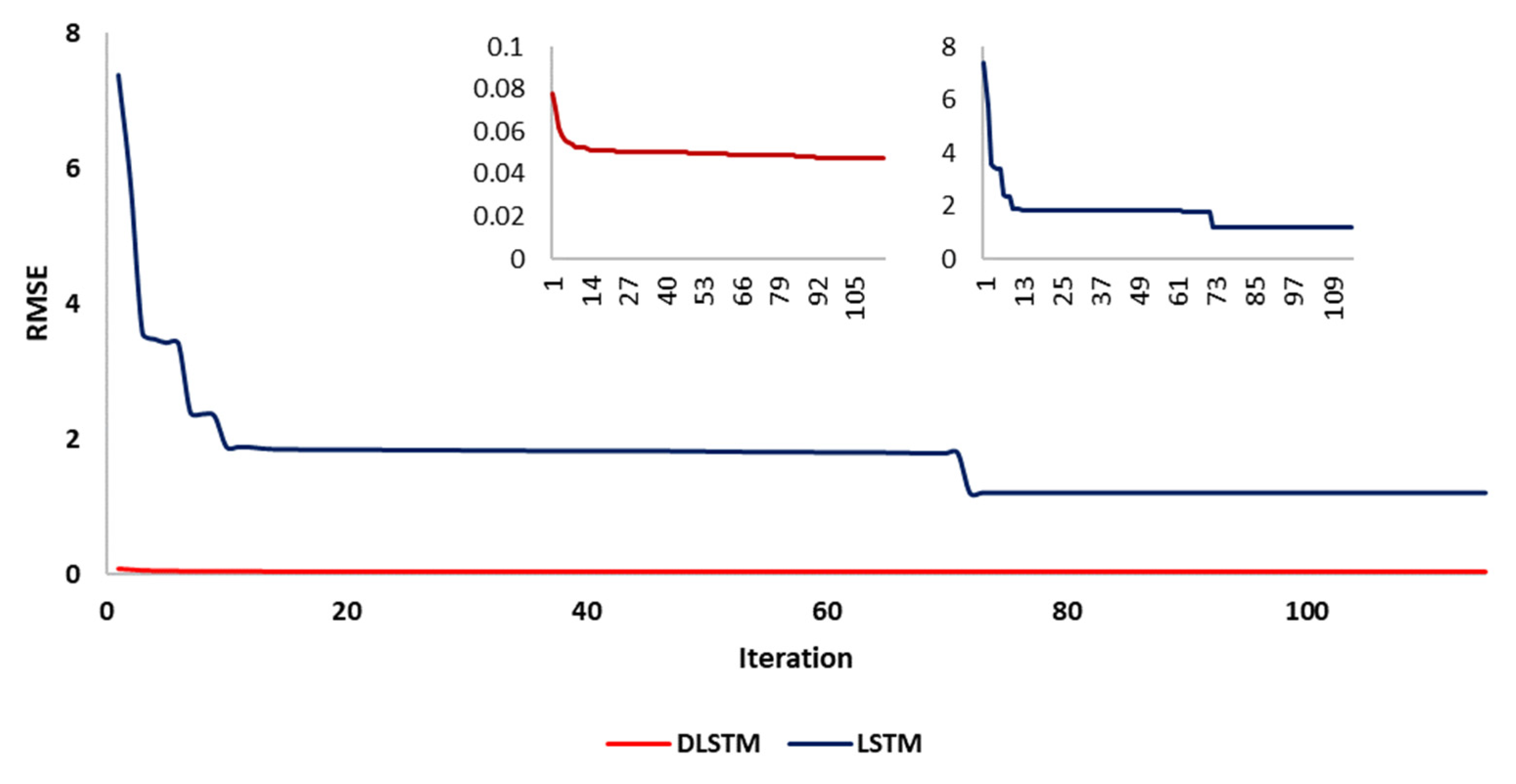
3. Results and Discussion

One of the prominent features of this article is the determination and prediction of daily temperature using powerful deep learning software, which has used consecutive time series data to determine this key parameter. This article utilizes 1097 data points gathered from the central and southern regions of Tabriz city of Iran in Asia from 2017 to 2019. The data was obtained from the world weather website. From 1079 datapoint, 70% of the dataset (768 data points) is used for the training dataset and 30% (329 data points) for the testing dataset. The input data related to the prediction of this critical parameter includes the time series Tt-3, Tt-2, and Tt-1. In other words, data related to three consecutive intervals (three consecutive days) makes it possible to predict the average air temperature obtained at time t.

To predict this error parameter, the data has been divided into two parts: training and testing. To divide the data, 70% of the data was used for training, and 30% was used for testing. The information related to the error parameters is used to check the criteria and compare the data related to test, train, and total (Equations (7) and (8)).

After determining the train data randomly, the desired LSTM deep learning algorithm has been developed and finally evaluated using the test data of this algorithm.

The results presented in this algorithm show the high accuracy of this algorithm compared to other algorithms for predicting this important environmental parameter. The following results are obtained by examining the results: the performance accuracy of the deep learning algorithm for train and test data is RMSE = 0.02 °C, R-Square = 0.99 and RMSE = 0.07 °C, R-Square = 0.99.

The results related to the information related to the test, the most, and the entire dataset are reported in

Table 2. Error parameter determination based on the train, test, and total dataset for prediction of daily temperature based on the developed LSTM deep learning model.

Models	Dataset	ARE (%)	AARE (%)	SD (°C)	RMSE SD (°C)	R-Square
LSTM	Train	0.12	0.06	1.05	1.06	0.94
	Test	−0.24	0.09	1.30	1.33	0.93
	Total	0.13	0.07	1.22	1.20	0.93
DLSTM	Train	−0.01	0.01	0.02	0.02	0.99
	Test	−0.04	0.04	0.08	0.08	0.99
	Total	−0.03	0.02	0.04	0.04	0.99

.

In evaluating the accuracy of the machine and deep learning algorithms in predicting a data point, root mean squared error (RMSE) and R-squared are widely recognized as two of the most commonly used validation factors. The RMSE metric provides an estimation of the average difference between the predicted values and actual values, making it a useful tool for assessing the performance of a model. On the other hand, R-squared measures the amount of variance in the target variable that can be explained by the model and is therefore indicative of the model’s explanatory power.

Overall, RMSE and R-squared are critical measures for assessing the efficacy of machine and deep learning algorithms in various applications such as image recognition, natural language processing, and financial forecasting. In addition, they are essential for identifying the strengths and limitations of a given model, as well as for comparing and selecting between different models. By providing a quantitative and systematic evaluation of model performance, these metrics contribute to improving the accuracy and reliability of predictions made by machine learning algorithms. It is, therefore, essential for researchers and practitioners to pay attention to these measures when designing, implementing, and evaluating machine and deep learning algorithms.

The results of the comparison of validation factors between LSTM and DLSTM deep learning models are displayed in Figure 6. The figure presents a comparison of two commonly used validation factors, RMSE and R-square, which are useful for evaluating the accuracy and performance of machine learning algorithms in predicting a data point. The findings in Figure 6 reveal that the DLSTM algorithm demonstrates superior performance compared to LSTM in terms of both RMSE and R-square values. Specifically, DLSTM shows lower RMSE values and higher R-square values, indicating higher accuracy and better explanatory power of the model.

These results suggest that DLSTM could be a better option for applications that require accurate predictions and efficient performance. In particular, the superior performance of DLSTM in both RMSE and R-square values can be attributed to its ability to learn complex patterns and dependencies in the input data, enabling it to generate more accurate predictions.

The significance of these findings extends beyond the field of deep learning and has implications for various applications, including image recognition, speech recognition, and natural language processing. By providing accurate and efficient predictions, DLSTM can contribute to the development of more advanced and reliable machine learning systems. Further research could be conducted to explore the performance of DLSTM in different contexts and datasets, as well as to compare it with other deep learning models. This can help provide a more comprehensive understanding of the capabilities and limitations of DLSTM and contribute to the advancement of the field of deep learning.

Based on the reports shown in Table 2, it is possible to understand the high accuracy of this algorithm. One of the characteristics of cross-plot diagrams is the accuracy of the performance of the algorithms. Using the cross points between measured and predicted, the accuracy of the performance can be observed visually. This statical parameter value can be obtained using the R-square mathematical relationship, among other chart features. As can be seen in Figure 7, the R-square information for the entire dataset is 0.99 for this DLSTM. After the checks shown in Figure 7, it is clear that DLSTM is better than the LSTM model. LSTM and DLSTM are two recurrent neural networks frequently utilized for time series prediction and sequence modeling. Although these models have comparable architecture, their primary distinction is the number of layers. LSTM has only one layer, while DLSTM has multiple layers. This enables DLSTM to identify more intricate patterns in the data and produce more precise forecasts. These figures clearly show that the LSTM algorithm contains more outlier data, but this new DLSTM model has higher accuracy, and outlier data is closer to the trendline.

The information related to Figure 8, which is related to the determination of prediction and measurement of daily temperature based on the (a) LSTM and (b) developed LSTM (DLSTM) deep learning models, was used to check the distance between the measured and predicted temperature. This chart is arranged based on the temperature order from low to high. According to the investigations carried out in this article, the performance accuracy of the measured and predicted data for determining the air temperature is very close to each other and has a higher accuracy. Preliminary tests show that this algorithm has a higher performance accuracy. Based on the graphical results seen in Figure 8, the accuracy of the DLSTM algorithm is much better than LSTM. After checking, we concluded that this algorithm’s performance accuracy is very high and has a very high performance. These figures provide a detailed comparison of these two algorithms as well as confirmation of the output of these two algorithms. These numbers show that the new algorithm is more accurate than the existing algorithms.

One way to determine an algorithm’s performance accuracy based on the number of iterations is to use iteration charts based on the amount of error (RMSE) (shown in Figure 9). For the DLSTM model, the error is high in the initial iterations and converges quickly when it reaches iteration 4. This figure shows that these error levels in iteration 68 have great performance accuracy and are quite near to one another. The performance accuracy for iteration 100 is finally RMSE = 0.04735 C. As a result, this error is mentioned as the last error for the total data. For the LSTM model, the error first starts from RMSE = 7 C for iteration = 1, and the reduction of the RMSE error starts from iteration = 7. In iteration = 72, it has a decrease equal to RMSE = 1.20 C. After examining two models, LSTM and DLSTM, it is clear that the accuracy of DLSTM is much higher.

LSTM and DLSTM are both types of recurrent neural networks that are used for predicting data points. However, there are some key differences between the two. LSTM is a type of neural network designed to handle sequential data. It is beneficial for predicting time series data, such as stock prices or weather patterns. LSTM networks have a memory cell that can store information over time, allowing the network to remember important patterns in the data. DLSTM, on the other hand, is a more complex version of LSTM that includes multiple layers of memory cells. This allows the network to learn more complex patterns in the data and make more accurate predictions. DLSTM networks are beneficial for predicting complex sequences of events, such as speech recognition or natural language processing. In summary, while both LSTM and DLSTM are used for predicting data points, DLSTM is a more advanced version that includes multiple layers of memory cells and is better suited for handling complex sequences of events.

4. Conclusions

This study used and compared two models, the LSTM and DLSTM neural network deep learning models, to predict the daily air temperature in Asia. This article utilizes 1097 data points gathered from the central and southern regions of Tabriz city of Iran in Asia from 2017 to 2019. The data was obtained from the world weather website. The input data related to the prediction of this critical parameter includes the time series Tt-3, Tt-2, and Tt-1. The daily air temperature is predicted using the air temperature using DLSTM and LSTM neural network model. LSTM and DLSTM are both types of recurrent neural networks that are used for predicting data points.

However, there are some key differences between the two. LSTM is a type of neural network designed to handle sequential data. It is particularly useful for predicting time series data, such as stock prices or weather patterns. LSTM networks have a memory cell that can store information over time, allowing the network to remember important patterns in the data. DLSTM, on the other hand, is a more complex version of LSTM that includes multiple layers of memory cells. This allows the network to learn more complex patterns in the data and make more accurate predictions. DLSTM networks are particularly useful for predicting complex sequences of events, such as speech recognition or natural language processing.

In summary, while both LSTM and DLSTM are used for predicting data points, DLSTM is a more advanced version that includes multiple layers of memory cells and is better suited for handling complex sequences of events. The proposed model in this study remarkably predicts the daily air temperature and the air temperature for the test data as RMSE = 0.08 °C, R-Square = 0.99. Therefore, this model can be used in future studies due to its remarkable accuracy in predicting air temperature.

References

1. Tol, R.S.J. Estimates of the damage costs of climate change, Part II. Dynamic estimates. Environ. Resour. Econ. 2002, 21, 135–160. [Google Scholar] [CrossRef]
2. Thober, S.; Kumar, R.; Wanders, N.; Marx, A.; Pan, M.; Rakovec, O.; Samaniego, L.; Sheffield, J.; Wood, E.F.; Zink, M. Multi-model ensemble projections of European river floods and high flows at 1.5, 2, and 3 degrees global warming. Environ. Res. Lett. 2018, 13, 014003. [Google Scholar] [CrossRef]
3. Van Vliet, M.T.H.; Franssen, W.H.P.; Yearsley, J.R.; Ludwig, F.; Haddeland, I.; Lettenmaier, D.P.; Kabat, P. Global river discharge and water temperature under climate change. Glob. Environ. Chang. 2013, 23, 450–464. [Google Scholar] [CrossRef]
4. Pearson, R.G.; Dawson, T.P. Predicting the impacts of climate change on the distribution of species: Are bioclimate envelope models useful? Glob. Ecol. Biogeogr. 2003, 12, 361–371. [Google Scholar] [CrossRef] [Green Version]
5. Bale, J.S.; Masters, G.J.; Hodkinson, I.D.; Awmack, C.; Bezemer, T.M.; Brown, V.K.; Butterfield, J.; Buse, A.; Coulson, J.C.; Farrar, J. Herbivory in global climate change research: Direct effects of rising temperature on insect herbivores. Glob. Chang. Biol. 2002, 8, 1–16. [Google Scholar] [CrossRef]
6. Canton, H. World Meteorological Organization—WMO. In The Europa Directory of International Organizations 2021; Routledge: London, UK, 2021; pp. 388–393. [Google Scholar]
7. World Meteorological Organization; World Health Organization (WHO). Heatwaves and Health: Guidance on Warning-System Development; WHO: Geneva, Switzerland, 2015. [Google Scholar]
8. Bate-Sproston, C. Sustainable Development Commission 2 (SDC2) Issue: Developing Heat Health Warning Systems in Countries Facing Heat Waves. In Proceedings of the Hague International Model United Nations (THIMUN The Hague), Hague, The Netherlands, 23–26 January 2023. [Google Scholar]
9. Williams, S.; Nitschke, M.; Weinstein, P.; Pisaniello, D.L.; Parton, K.A.; Bi, P. The impact of summer temperatures and heatwaves on mortality and morbidity in Perth, Australia 1994–2008. Environ. Int. 2012, 40, 33–38. [Google Scholar] [CrossRef]
10. Ebi, K.L.; Lewis, N.D.; Corvalan, C. Climate variability and change and their potential health effects in small island states: Information for adaptation planning in the health sector. Environ. Health Perspect. 2006, 114, 1957–1963. [Google Scholar] [CrossRef] [Green Version]
11. Xie, Y.; Fan, S.; Chen, M.; Shi, J.; Zhong, J.; Zhang, X. An assessment of satellite radiance data assimilation in RMAPS. Remote Sens. 2018, 11, 54. [Google Scholar] [CrossRef] [Green Version]
12. Shahzaman, M.; Zhu, W.; Ullah, I.; Mustafa, F.; Bilal, M.; Ishfaq, S.; Nisar, S.; Arshad, M.; Iqbal, R.; Aslam, R.W. Comparison of multi-year reanalysis, models, and satellite remote sensing products for agricultural drought monitoring over south asian countries. Remote Sens. 2021, 13, 3294. [Google Scholar] [CrossRef]
13. Gauer, R.L.; Meyers, B.K. Heat-related illnesses. Am. Fam. Physician 2019, 99, 482–489. [Google Scholar]
14. Iyakaremye, V.; Zeng, G.; Yang, X.; Zhang, G.; Ullah, I.; Gahigi, A.; Vuguziga, F.; Asfaw, T.G.; Ayugi, B. Increased high-temperature extremes and associated population exposure in Africa by the Mid-21st Century. Sci. Total Environ. 2021, 790, 148162. [Google Scholar] [CrossRef] [PubMed]
15. Ullah, I.; Saleem, F.; Iyakaremye, V.; Yin, J.; Ma, X.; Syed, S.; Hina, S.; Asfaw, T.G.; Omer, A. Projected changes in socioeconomic exposure to heatwaves in South Asia under changing climate. Earth’s Future 2022, 10, e2021EF002240. [Google Scholar] [CrossRef]
16. Tabasi, S.; Tehrani, P.S.; Rajabi, M.; Wood, D.A.; Davoodi, S.; Ghorbani, H.; Mohamadian, N.; Alvar, M.A. Optimized machine learning models for natural fractures prediction using conventional well logs. Fuel 2022, 326, 124952. [Google Scholar] [CrossRef]
17. Beheshtian, S.; Rajabi, M.; Davoodi, S.; Wood, D.A.; Ghorbani, H.; Mohamadian, N.; Alvar, M.A.; Band, S.S. Robust computational approach to determine the safe mud weight window using well-log data from a large gas reservoir. Mar. Pet. Geol. 2022, 142, 105772. [Google Scholar] [CrossRef]
18. Rajabi, M.; Hazbeh, O.; Davoodi, S.; Wood, D.A.; Tehrani, P.S.; Ghorbani, H.; Mehrad, M.; Mohamadian, N.; Rukavishnikov, V.S.; Radwan, A.E. Predicting shear wave velocity from conventional well logs with deep and hybrid machine learning algorithms. J. Pet. Explor. Prod. Technol. 2022, 13, 19–42. [Google Scholar] [CrossRef]
19. Kamali, M.Z.; Davoodi, S.; Ghorbani, H.; Wood, D.A.; Mohamadian, N.; Lajmorak, S.; Rukavishnikov, V.S.; Taherizade, F.; Band, S.S. Permeability prediction of heterogeneous carbonate gas condensate reservoirs applying group method of data handling. Mar. Pet. Geol. 2022, 139, 105597. [Google Scholar] [CrossRef]
20. Qian, Q.F.; Jia, X.J.; Lin, H. Machine learning models for the seasonal forecast of winter surface air temperature in North America. Earth Space Sci. 2020, 7, e2020EA001140. [Google Scholar] [CrossRef]
21. Novitasari, D.C.R.; Rohayani, H.; Junaidi, R.; Setyowati, R.D.N.; Pramulya, R.; Setiawan, F. Weather parameters forecasting as variables for rainfall prediction using adaptive neuro fuzzy inference system (ANFIS) and support vector regression (SVR). J. Phys. Conf. Ser. 2020, 1501, 012012. [Google Scholar] [CrossRef]
22. Hanoon, M.S.; Ahmed, A.N.; Zaini, N.a.; Razzaq, A.; Kumar, P.; Sherif, M.; Sefelnasr, A.; El-Shafie, A. Developing machine learning algorithms for meteorological temperature and humidity forecasting at Terengganu state in Malaysia. Sci. Rep. 2021, 11, 18935. [Google Scholar] [CrossRef]
23. Gad, I.; Hosahalli, D. A comparative study of prediction and classification models on NCDC weather data. Int. J. Comput. Appl. 2022, 44, 414–425. [Google Scholar] [CrossRef]
24. Katušić, D.; Pripužić, K.; Maradin, M.; Pripužić, M. A comparison of data-driven methods in prediction of weather patterns in central Croatia. Earth Sci. Inform. 2022, 15, 1249–1265. [Google Scholar] [CrossRef]
25. Essien, A.; Giannetti, C. A deep learning framework for univariate time series prediction using convolutional LSTM stacked autoencoders. In Proceedings of the 2019 IEEE International Symposium on Innovations in Intelligent Systems and Applications (INISTA), Sofia, Bulgaria, 3–5 July 2019; pp. 1–6. [Google Scholar]
26. Tsochantaridis, I.; Joachims, T.; Hofmann, T.; Altun, Y.; Singer, Y. Large margin methods for structured and interdependent output variables. J. Mach. Learn. Res. 2005, 6, 1453–1484. [Google Scholar]
27. Muralitharan, K.; Sakthivel, R.; Vishnuvarthan, R. Neural network based optimization approach for energy demand prediction in smart grid. Neurocomputing 2018, 273, 199–208. [Google Scholar] [CrossRef]
28. Brownlee, J. Deep Learning for Time Series Forecasting: Predict the Future with MLPs, CNNs and LSTMs in Python; Machine Learning Mastery: Victoria, Australia, 2018. [Google Scholar]
29. Gers, F.A.; Schmidhuber, J.; Cummins, F. Learning to forget: Continual prediction with LSTM. Neural Comput. 2000, 12, 2451–2471. [Google Scholar] [CrossRef] [PubMed]
30. Yu, Y.; Si, X.; Hu, C.; Zhang, J. A review of recurrent neural networks: LSTM cells and network architectures. Neural Comput. 2019, 31, 1235–1270. [Google Scholar] [CrossRef]
31. Dennis, J.B.; Misunas, D.P. A preliminary architecture for a basic data-flow processor. In Proceedings of the 2nd Annual Symposium on Computer Architecture, Houston, TX, USA, 1 December 1974; pp. 126–132. [Google Scholar]
32. Adam, K.; Smagulova, K.; James, A.P. Memristive LSTM network hardware architecture for time-series predictive modeling problems. In Proceedings of the 2018 IEEE Asia Pacific Conference on Circuits and Systems (APCCAS), Chengdu, China, 26–30 October 2018; pp. 459–462. [Google Scholar]
33. Liu, P.; Sun, X.; Han, Y.; He, Z.; Zhang, W.; Wu, C. Arrhythmia classification of LSTM autoencoder based on time series anomaly detection. Biomed. Signal Process. Control 2022, 71, 103228. [Google Scholar] [CrossRef]
34. Ji, Y.; Yamashita, A.; Asama, H. RGB-D SLAM using vanishing point and door plate information in corridor environment. Intell. Serv. Robot. 2015, 8, 105–114. [Google Scholar] [CrossRef]
35. Faghihi Nezhad, M.T.; Minaei Bidgoli, B. Development of an ensemble learning-based intelligent model for stock market forecasting. Sci. Iran 2021, 28, 395–411. [Google Scholar]
36. Sen, S.; Raghunathan, A. Approximate computing for long short term memory (LSTM) neural networks. IEEE Trans. Comput.-Aided Des. Integr. Circuits Syst. 2018, 37, 2266–2276. [Google Scholar] [CrossRef]
37. Kim, T.; Kim, H.Y. Forecasting stock prices with a feature fusion LSTM-CNN model using different representations of the same data. PLoS ONE 2019, 14, e0212320. [Google Scholar] [CrossRef] [Green Version]
38. Mustafaraj, G.; Lowry, G.; Chen, J. Prediction of room temperature and relative humidity by autoregressive linear and nonlinear neural network models for an open office. Energy Build. 2011, 43, 1452–1460. [Google Scholar] [CrossRef]
39. Xie, J.; Wang, Q. Benchmark machine learning approaches with classical time series approaches on the blood glucose level prediction challenge. CEUR Workshop Proc. 2018, 2148, 97–102. [Google Scholar]
40. Tsangaratos, P.; Ilia, I. Comparison of a logistic regression and Naïve Bayes classifier in landslide susceptibility assessments: The influence of models complexity and training dataset size. Catena 2016, 145, 164–179. [Google Scholar] [CrossRef]
41. Shin, H.-C.; Roth, H.R.; Gao, M.; Lu, L.; Xu, Z.; Nogues, I.; Yao, J.; Mollura, D.; Summers, R.M. Deep convolutional neural networks for computer-aided detection: CNN architectures, dataset characteristics and transfer learning. IEEE Trans. Med. Imaging 2016, 35, 1285–1298. [Google Scholar] [CrossRef] [PubMed] [Green Version]
42. Xiong, Z.; Cui, Y.; Liu, Z.; Zhao, Y.; Hu, M.; Hu, J. Evaluating explorative prediction power of machine learning algorithms for materials discovery using k-fold forward cross-validation. Comput. Mater. Sci. 2020, 171, 109203. [Google Scholar] [CrossRef]
43. Barrow, D.K.; Crone, S.F. Crogging (cross-validation aggregation) for forecasting—A novel algorithm of neural network ensembles on time series subsamples. In Proceedings of the 2013 International Joint Conference on Neural Networks (IJCNN), Dallas, TX, USA, 4–9 August 2013; pp. 1–8. [Google Scholar]
44. Rossi, F.; Lendasse, A.; François, D.; Wertz, V.; Verleysen, M. Mutual information for the selection of relevant variables in spectrometric nonlinear modelling. Chemom. Intell. Lab. Syst. 2006, 80, 215–226. [Google Scholar] [CrossRef] [Green Version]
45. Lahiri, S.K.; Ghanta, K.C. Regime identification of slurry transport in pipelines: A novel modelling approach using ANN & differential evolution. Chem. Ind. Chem. Eng. Q. 2010, 16, 329–343. [Google Scholar]
46. Deng, L.; Yu, D. Deep learning: Methods and applications. Found. Trends® Signal Process. 2014, 7, 197–387. [Google Scholar] [CrossRef] [Green Version]
47. Chen, L.-C.; Papandreou, G.; Schroff, F.; Adam, H. Rethinking atrous convolution for semantic image segmentation. arXiv 2017, arXiv:1706.05587. [Google Scholar]
48. Breuel, T.M. The effects of hyperparameters on SGD training of neural networks. arXiv 2015, arXiv:1508.02788. [Google Scholar]
Figure 1. Illustration of dataset conversion in a sliding window of length N.
Sustainability 15 09289 g001
Figure 2. Partial view of L cell structure.
Sustainability 15 09289 g002
Figure 3. The architecture of the first model.
Sustainability 15 09289 g003
Figure 4. The architecture of the second model.
Sustainability 15 09289 g004
Figure 5. Validation of time series data.
Sustainability 15 09289 g005
Figure 6. Comparison of common validation factors (RMSE and R-square) between LSTM and DLSTM deep learning models.
Sustainability 15 09289 g006
Figure 7. Cross plot for prediction versus daily temperature measurement based on (a) LSTM and (b) developed LSTM (DLSTM) deep learning models.
Sustainability 15 09289 g007aSustainability 15 09289 g007b
Figure 8. Determination of prediction and measurement of daily temperature based on the (a) LSTM and (b) developed LSTM (DLSTM) deep learning models.
Sustainability 15 09289 g008aSustainability 15 09289 g008b
Figure 9. Illustration of iteration based on the error parameter for developed LSTM deep learning.
Sustainability 15 09289 g009