Artificial Intelligence and Urban Green Space Facilities Optimization Using the LSTM Model: Evidence from China

Abstract

Urban road green belts, an essential component of Urban Green Space (UGS) planning, are vital in improving the urban environment and protecting public health. This work chooses Long Short-Term Memory (LSTM) to optimize UGS planning and design methods in urban road green belts. Consequently, sensitivity-based self-organizing LSTM shows a Root Mean Square Error (RMSE), Mean Absolute Error (MAE), and Mean Absolute Percentage Error (MAPE) of 1.75, 1.12, and 6.06, respectively. These values are superior to those of LSTM, XGBoost, and SVR. Furthermore, we configure three typical plant community models using the improved LSTM model and found that different plant community configurations have distinct effects on reducing PM 2.5 concentrations. The experimental results show that other plant community configuration models have specific effects on reducing PM 2.5 concentrations, and the multi-layered green space with high canopy density in the community has a better impact on PM 2.5 reduction than the single-layer green space model with low canopy density. We also assess the reduction function of green road spaces on PM 2.5, which revealed that under zero pollution or slight pollution (PM 2.5 < 100 μg.m⁻³), the green space significantly reduces PM 2.5. In UGS planning, the proposed model can help reveal UGS spatial morphology indicators that significantly impact PM 2.5 reduction, thereby facilitating the formulation of appropriate green space planning strategies. The finding will provide primary data for selecting urban road green space plant configuration.

1. Introduction

With continuous socioeconomic development and improved living standards, urban modernization paces up, and private car ownership substantially grows. However, this has also given rise to various urban issues, like environmental pollution, of which the hazy weather affects urban residents’ lives most directly [1,2]. In particular, Particulate Matter 2.5 (PM 2.5) particles are the main component of smog, particles in the ambient air with an equivalent aerodynamic diameter of 2.5 microns or less. Of these, larger-sized PM 2.5 particles can adsorb harmful substances and bypass the human body’s immune system. Eventually, they will adhere to and invade the respiratory tract and pulmonary lobes, reducing the defense function of the human respiratory system. It can also weaken near-ground ultraviolet rays, enhancing in-air infectious bacteria’s vitality and increasing contagious diseases. In haze conditions, individuals who breathe more frequently and deeply are at a higher risk of inhaling more significant amounts of harmful substances into their bodies. These can induce or exacerbate various diseases. The direct results are the subjects’ poor breathing, eye irritation, chest tightness, chest pain, headache, dry throat itching, cough, and vomiting. Elderly patients with a history of chronic bronchitis, asthma, or chronic respiratory diseases, can easily suffer acute upper respiratory tract infections, rhinitis, acute bronchitis, chronic bronchitis, asthma, and pneumonia attacks. Therefore, hazy weather can damage human cells and prevent them from functioning normally, damaging the human’s physical and mental health. PM pollution can also cause severe losses to tourism, agriculture, social order, and ecosystems [3]. To this end, many experts devised ways to monitor and predict air quality. Currently, air quality prediction models employ either numerical prediction based on atmospheric kinematics or statistical approaches based on Machine Learning algorithms. The numerical prediction model is based on the internal physical laws of the atmosphere, such as atmospheric dynamics and thermodynamics, to establish corresponding mathematical and physical models relying on mathematical methods and the computing power of large-scale computers. Numerical prediction models factor in the dynamic distribution, transportation, and diffusion of air pollutant concentrations. Machine Learning models use statistics, probability theory, and complex algorithms to build models, mine data relationships from known data, and achieve refined predictions. Ecologists initially proposed the concept of Sustainable Development (SD) as a development plan that can meet contemporary needs without adversely affecting future generations. The aim is to balance the development of natural ecological resources. Subsequently, experts in various fields began to define SD in terms of social, economic, and technological attributes. Ultimately, achieving Sustainable Development (SD) hinges on coordinating and integrating social, economic, population, resources, and environmental development efforts. So far, research on SD mainly draws on academic attempts in different academic fields, with much information scattered or heterogeneous. A sustainable economy has emerged as the engine for the era’s continued growth in light of the global economy’s quick expansion [4]. Continuous social development will likely drive much information interleaving and fusion. Regarding the big data of scientific research, applying SD to the scientific field can improve the information utilization rate and promote sustainable science and technological development.

Researchers have done much research work in corresponding fields. For example, Yin (2020) [5,6] studied the characteristics of Urban Green Space (UGS) under shared transportation. They proposed strategies for urban spatial planning in China, such as activating spatial inventory, road sharing, and establishing a credit system. Zhang et al. (2020) [7,8] pointed out that UGS, a natural-based solution for promoting public health, provided cities with a wide range of ecosystem services. They believed UGS was conducive to promoting the SD of cities and improving residents’ life quality. The author proposed a theoretical framework and summarized the potential ways for UGS to provide health benefits from four perspectives: encouraging physical activity, alleviating psychological stress, providing environmental regulation and support services, and promoting social cohesion. Then, combined with theoretical review research, a preliminary health-based UGS planning and design strategy was proposed. Shan et al. (2021) [9,10] contended that UGS, a key component of urban infrastructure, should be upgraded with the Smart City construction. Intelligent UGS (Unigraphics) planning and sustainable landscaping schemes would fuse UGS’s ecological performance and similar functions. Intelligent unattended ground sensor planning was a technological approach and a human-oriented smart application. They proposed an ensemble UGS segmentation model based on five types of unattended ground sensors from sample stations in Baqiao District, the City of Xi’an, Shaanxi Province. They conducted a survey to assess the socioeconomic attributes of respondents, as well as differences in their access frequency and demand for the services under investigation. Finally, the UGS under study was improved based on public preferences and the station’s current conditions. Wang et al. (2023) [11,12] suggested that by drawing upon the experience of green development in the existing pilot cities, the government could broaden the pilot’s scope and reinforce its policy orientation towards green development, thus facilitating sustainable development in the cities. Zou and Wang (2021) [13,14] argued that a morphological perspective was a novel way to carry out UGS planning practices, protect and restore urban natural habitat functions, and maintain an excellent spatial pattern of the ecological environment. With respect to the investigation and analysis of relevant scientific literature on UGS morphology, their research discussed the regional and temporal background of UGS morphology research, as well as the knowledge framework of related research. The existing problems in UGS morphology research have also been revealed. Based on this, it proposed future research directions and objectives. Notably, the extant scholarship predominantly focuses on the urban scale, with some quantitative research results, and needs an in-depth quantitative and detailed analysis of green patches.

The significance of this work is based on the fact that the harmful effect of PM 2.5 has recently attracted widespread attention. This work quantifies the impact of UGS on air quality from the perspective of PM 2.5 reduction, enriching the theories and methods of UGS planning and design. This work aims to deepen research on urban infrastructure in the ecological direction. By studying the planning and design of UGS to regulate PM 2.5 pollution, the research system of PM 2.5 has been enriched. This work begins with a quantitative study of the impact of different morphological characteristics of UGS on the internal PM 2.5 concentration and the degree of impact of different types of UGS on surrounding PM 2.5. It supplements the systematic quantitative study of the current preliminary phenomenon description. The PM 2.5 concentration in xx city was chosen as the research object, and the Long Short-Term Memory (LSTM) model was introduced to forecast the PM 2.5 concentration. Then, to solve the network structure problem, a sensitivity-based self-organizing LSTM is proposed for PM 2.5 concentration prediction. Finally, UGS planning is conducted based on the predicted PM 2.5 concentration in different regions of xx city.

2. Algorithms for Predicting PM 2.5 Concentration Based on Neural Networks

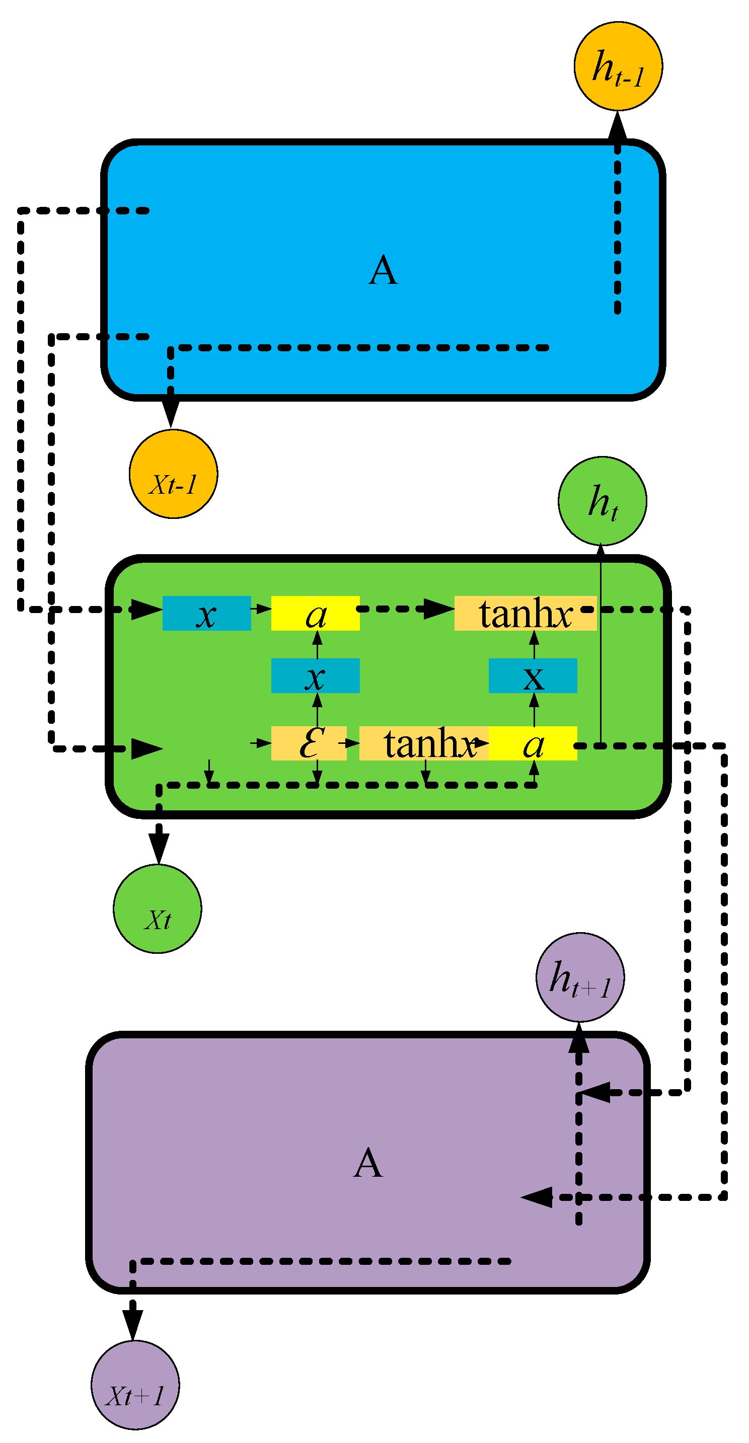
2.1. RNN and LSTM Algorithm

As a typical Feed Forward Neural Network (FNN), Recurrent Neural Network (RNN)s differ from FNNs. While an FNN’s neurons only transfer information between layers, an RNN allows information to be transferred between neurons by introducing a circular structure [15,16,17]. In this way, RNN can memorize the last input as a “storage” and provide a reference for the following step [18,19,20,21,22]. Unlike an FNN, which can only map a hidden layer-to-output layer input, an RNN can map all information to an individual output neuron with a better prediction. An RNN model includes three layers: input, hidden, and output. The mathematical model of the RNN is shown in Equations (1)–(5):

$${\mathrm{h}}^{\left(\mathrm{t}\right)}=\mathsf{\phi }\left(\mathrm{U}{\mathrm{x}}^{\left(\mathrm{t}\right)}+\mathrm{W}{\mathrm{h}}^{(\mathrm{t}-1)}+\mathrm{b}\right)$$

(1)

$${\mathrm{o}}^{\left(\mathrm{t}\right)}=\mathrm{V}{\mathrm{h}}^{\left(\mathrm{t}\right)}+\mathrm{c}$$

(2)

$${\widehat{\mathrm{y}}}^{\left(\mathrm{t}\right)}=\mathsf{\sigma }\left({\mathrm{o}}^{\left(\mathrm{t}\right)}\right)$$

(3)

$$\mathsf{\phi }\left(\mathrm{x}\right)=\frac{{\mathrm{e}}^{\mathrm{x}}-{\mathrm{e}}^{-\mathrm{x}}}{{\mathrm{e}}^{\mathrm{x}}+{\mathrm{e}}^{-\mathrm{x}}}$$

(4)

$${\mathrm{y}}^{\left(\mathrm{t}\right)}={\mathrm{o}}^{\left(\mathrm{t}\right)}$$

(5)

In Equations (1)–(5), $\mathrm{t}$ is the time point, ${\mathrm{x}}^{\left(\mathrm{t}\right)}$ and ${\mathrm{y}}^{\left(\mathrm{t}\right)}$ are the input quantities of the RNN’s input layer, and ${\mathrm{h}}^{\left(\mathrm{t}\right)}$ and ${\mathrm{h}}^{(\mathrm{t}-1)}$ represent the hidden layer outputs for the RNN at times $\mathrm{t}$ and $\mathrm{t}-$1, respectively. The $\mathsf{\phi }$ function activates the RNN’s hidden layer. ${\mathrm{o}}^{\left(\mathrm{t}\right)}$ and $\mathsf{\sigma }$ denote the input quantity and activation function of the RNN’s output layer, respectively. $\mathrm{U}$ denotes the weighted value from the input layer to the hidden layer. $\mathrm{W}$ and $\mathrm{b}$ mean the weight and bias between each hidden layer, respectively. Finally, $\mathrm{V}$ and $\mathrm{c}$ are the hidden layer-output layer weight and bias, respectively.

LSTM is a sub-category of RNN [23,24,25,26,27] and can effectively handle time series-dependent events. An LSTM unit contains one input gate and one output gate but multiple forgetting gates [28,29,30,31,32,33]. The input gate can control the model’s input data. The output gate functions as the model’s output controller for the calculation results. The forgetting gate helps determine what the memory module should forget (abandon) from the previous moment. The model structure is shown in Figure 1 and is calculated by Equation (6):

$${\mathrm{f}}_{\mathrm{t}}=\mathsf{\sigma }\left({\mathrm{W}}_{\mathrm{f}}\cdot \left[{\mathrm{h}}_{\mathrm{t}-1},{\mathrm{x}}_{\mathrm{t}}\right])+{\mathrm{b}}_{\mathrm{f}}\right.$$

(6)

Figure 1. Schematic diagram of LSTM structure.

In Equation (6), ${\mathrm{f}}_{\mathrm{t}}$ indicates a forgetting gate, which controls what input information to “forget,” and the input gate controls which new data to be written into long-term memory.

$${\mathrm{i}}_{\mathrm{t}}=\mathsf{\sigma }\left({\mathrm{W}}_{\mathrm{i}}\cdot \left[{\mathrm{h}}_{\mathrm{t}-1},{\mathrm{x}}_{\mathrm{t}}\right])+{\mathrm{b}}_{\mathrm{i}}\right.$$

(7)

$$\mathrm{C}=\mathrm{t}\mathrm{a}\mathrm{n}\mathrm{h}\left({\mathrm{W}}_{\mathrm{c}}\cdot \left[{\mathrm{h}}_{\mathrm{t}-1},{\mathrm{x}}_{\mathrm{t}}\right])+{\mathrm{b}}_{\mathrm{c}}\right.$$

(8)

$${\mathrm{C}}_{\mathrm{t}}={\mathrm{f}}_{\mathrm{t}}\times {\mathrm{C}}_{\mathrm{t}-1}+{\mathrm{i}}_{\mathrm{t}}\times \mathrm{C}$$

(9)

In Equations (7)–(9), ${\mathrm{i}}_{\mathrm{t}}$ represents an input gate. ${\mathrm{f}}_{\mathrm{t}}$ and ${\mathrm{i}}_{\mathrm{t}}$ choose the Sigmoid activation function. When the Sigmoid function outputs between 0 and 1, ${\mathrm{C}}_{\mathrm{t}-1}$ and ${\mathrm{C}}_{\mathrm{t}}$ represent the neuron’s t − 1-moment and t-moment states, respectively.

$${\mathrm{h}}_{\mathrm{t}}={\mathrm{o}}_{\mathrm{t}}\times \mathrm{t}\mathrm{a}\mathrm{n}\mathrm{h}\left({\mathrm{C}}_{\mathrm{t}}\right)$$

(10)

$${\mathrm{o}}_{\mathrm{t}}=\mathsf{\sigma }\left({\mathrm{w}}_{\mathrm{o}}\cdot \left[{\mathrm{h}}_{\mathrm{t}-1},{\mathrm{x}}_{\mathrm{t}}\right])+{\mathrm{b}}_{\mathrm{o}}\right.$$

(11)

In Equation (11), ${\mathrm{o}}_{\mathrm{t}}$ is the output gate control signal’s output level. ${\mathrm{w}}_{\mathrm{o}}$ denotes the sequence’s output at the tth step.

Figure 2 shows an improved LSTM.

Figure 2. An improved LSTM.

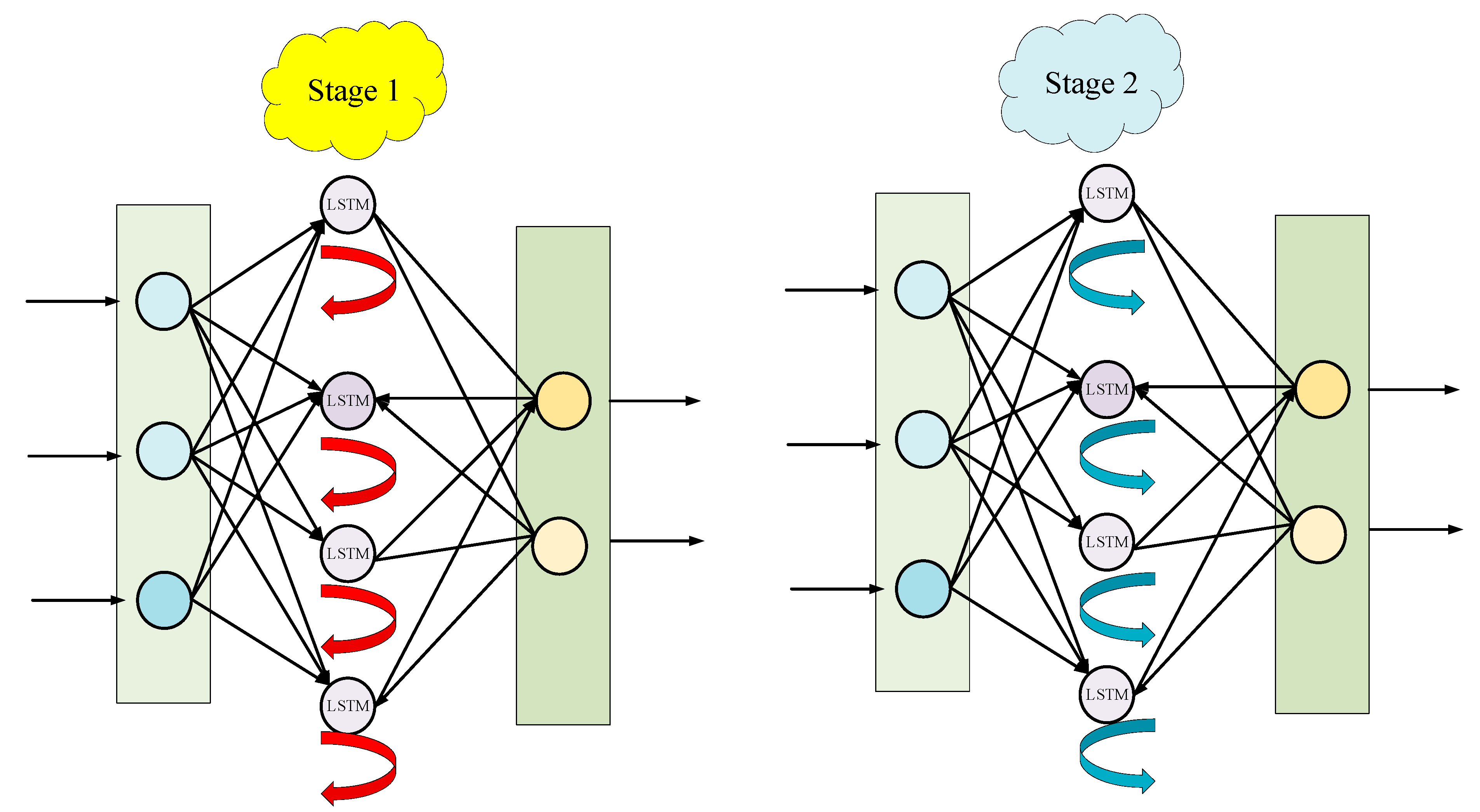
2.2. Prediction Algorithm Based on Self-Organizing LSTM

This section introduces a sensitivity-based algorithm for self-organizing training of LSTM. The decomposition of the LSTM network is shown in Figure 3. Here, the red arrow represents the self-feedback portion of the hidden layer neuron [34,35], which is the output of the hidden layer neuron at $\mathrm{t}-1$ time (expressed as ${\mathrm{z}}_1\left(\mathrm{t}\right)=\left({\mathrm{H}}_1(\mathrm{t}-1),{\mathrm{H}}_2(\mathrm{t}-1),\cdots ,{\mathrm{H}}_{\mathrm{N}}(\mathrm{t}-1)\right)$) where $\mathrm{N}$ represents the number of neurons in the hidden layer. The blue arrow indicates the output portion from the hidden layer to the output layer, that is, the output of the hidden layer neuron at time $\mathrm{t}$ (expressed as ${\mathrm{z}}_2\left(\mathrm{t}\right)=\left({\mathrm{H}}_1\left(\mathrm{t}\right),{\mathrm{H}}_2\left(\mathrm{t}\right),\cdots ,{\mathrm{H}}_{\mathrm{N}}\left(\mathrm{t}\right)\right)$).

Figure 3. LSTM decomposition diagram.

The sensitivity of the self-organizing LSTM is defined by Equation (12):

$${\mathrm{S}}_{\mathrm{h}}=\frac{\mathrm{Var}\left[\mathrm{E}\left(\mathrm{Y}\mid {\mathrm{Z}}_{\mathrm{h}}\right)\right]}{\mathrm{Var}\left(\mathrm{Y}\right)},\left(\mathrm{h}=1,2,\cdots ,\mathrm{N}\right)$$

(12)

In Equation (12), ${\mathrm{Z}}_{\mathrm{h}}$ represents the $\mathrm{h}$th input factor, $\mathrm{Y}$ is the output layer output of the model and $\mathrm{E}\left(\mathrm{Y}\mid {\mathrm{Z}}_{\mathrm{h}}\right)$ means the expected output of the constant ${\mathrm{Z}}_{\mathrm{h}}$ under the condition of $\mathrm{Y}$. $\mathrm{V}\mathrm{a}\mathrm{r}\left(\right)$ means the calculated variance.

In this work, the proposed LSTM model divides the sensitivity analysis into two calculation parts: indirect sensitivity and direct sensitivity. The red self-feedback section in Figure 3 is used to calculate indirect sensitivity, while the blue output section is used to calculate direct sensitivity. Therefore, according to Equation (12), the calculation for indirect sensitivity reads:

$${\mathrm{S}}_{\mathrm{h}}^1\left(\mathrm{t}\right)=\frac{{\mathrm{Var}}_{\mathrm{h}}\left[\mathrm{E}\left(\mathrm{y}\left(\mathrm{t}\right)\right)\mid {\mathrm{Z}}_{\mathrm{h}}^1={\mathrm{H}}_{\mathrm{h}}\left(\mathrm{t}-1\right)\right]}{\mathrm{Var}\left[\mathrm{y}\left(\mathrm{t}\right)\right]}$$

(13)

In Equation (13), ${\mathrm{H}}_{\mathrm{h}}(\mathrm{t}-1)$ represents the output of the $\mathrm{h}$th hidden layer neuron at time ${\mathrm{H}}_{\mathrm{h}}(\mathrm{t}-1)$, namely the self-feedback of the $\mathrm{h}$th hidden layer neuron at time $\mathrm{t}$. By comparison, $\mathrm{y}\left(\mathrm{t}\right)$ denotes the output of the network output layer. According to Equation (13), the mathematical expression of ${\mathrm{H}}_{\mathrm{h}}(\mathrm{t}-1)$ reads:

$$\begin{array}{c}{\mathrm{H}}_{\mathrm{h}}\left(t\right)={\mathrm{h}}_{\mathrm{t}}\left(\mathrm{c}{\mathrm{c}}^{\mathrm{\text{'}}}\right){\mathrm{f}}_{\mathrm{t}}\left({\mathrm{Z}}_{\mathrm{o}}\right)\hfill \\ =h\left(\begin{array}{c}g\left({\mathrm{W}}_{\mathrm{x}}\cdot \left[{\mathrm{H}}_{\mathrm{h}}(\mathrm{t}-1),{\mathrm{x}}_{\mathrm{t}}\right]+{\mathrm{b}}_{\mathrm{x}}\right)f\left({\mathrm{W}}_{\mathrm{i}}\cdot \left[{\mathrm{H}}_{\mathrm{h}}(\mathrm{t}-1),{\mathrm{x}}_{\mathrm{t}}\right]+{\mathrm{b}}_{\mathrm{i}}\right)\\ +cf\left({\mathrm{W}}_{\mathrm{f}}\cdot \left[{\mathrm{H}}_{\mathrm{h}}(\mathrm{t}-1),{\mathrm{x}}_{\mathrm{t}}\right]+{\mathrm{b}}_{\mathrm{f}}\right)\end{array}\right)\hfill \\ +f\left({\mathrm{W}}_{\mathrm{o}}\cdot \left[{\mathrm{H}}_{\mathrm{h}}(\mathrm{t}-1),{\mathrm{x}}_{\mathrm{t}}\right]+{\mathrm{b}}_{\mathrm{o}}\right)\hfill \end{array}$$

(14)

In Equation (14), ${\mathrm{W}}_{\mathrm{x}},{\mathrm{W}}_{\mathrm{i}},{\mathrm{W}}_{\mathrm{f}},{\mathrm{W}}_{\mathrm{o}}$ represents the input weight of the LSTM unit, the weighted input gate, the forgetting gate, and the output gate’s control signals, respectively. ${\mathrm{b}}_{\mathrm{x}},{\mathrm{b}}_{\mathrm{i}},{\mathrm{b}}_{\mathrm{f}},{\mathrm{a}\mathrm{n}\mathrm{d}\mathrm{b}}_{\mathrm{o}}$ are the input bias, the bias of the input gate control signal, the bias of the forgetting gate control signal, and the bias of the output gate control signal, respectively.

The output representation of the output layer is shown in Equation (15):

$$\mathrm{y}\left(\mathrm{t}\right)=\sum _{\mathrm{j}=1}^{\mathrm{N}} {\mathrm{W}}_{\mathrm{j}}\left(\mathrm{t}\right){\mathrm{H}}_{\mathrm{j}}\left(\mathrm{t}\right)$$

(15)

In Equation (15), ${\mathrm{W}}_{\mathrm{j}}\left(\mathrm{t}\right)$ represents the weight connecting the $\mathrm{j}$th hidden layer neuron to the output layer at time $\mathrm{t}$.

The calculation method of direct sensitivity reads:

$${\mathrm{S}}_{\mathrm{h}}^2\left(\mathrm{t}\right)=\frac{{\mathrm{Var}}_{\mathrm{h}}\left[\mathrm{E}\left(\mathrm{y}\left(\mathrm{t}\right)\right)\mid {\mathrm{Z}}_{\mathrm{h}}^2={\mathrm{H}}_{\mathrm{h}}\left(\mathrm{t}\right)\right]}{\mathrm{Var}\left[\mathrm{y}\left(\mathrm{t}\right)\right]}$$

(16)

Direct sensitivity and indirect sensitivity have some differences. For direct sensitivity, the condition for obtaining the desired output is replaced by the output of the $\mathrm{h}$th hidden layer neuron at time $\mathrm{h}$, and this relationship is shown in Equation (17):

$$\begin{array}{c}{\mathrm{H}}_{\mathrm{h}}\left(t\right)={\mathrm{h}}_{\mathrm{t}}\left({\mathrm{c}}^{\mathrm{\text{'}}}\right){\mathrm{f}}_{\mathrm{t}}\left({\mathrm{Z}}_{\mathrm{o}}\right)\hfill \\ =h\left(\begin{array}{c}g\left({\mathrm{W}}_{\mathrm{x}}\cdot \left[{\mathrm{H}}_{\mathrm{h}}\left(\mathrm{t}-1\right),{\mathrm{x}}_{\mathrm{t}}\right]+{\mathrm{b}}_{\mathrm{x}}\right)f\left({\mathrm{W}}_{\mathrm{i}}\cdot \left[{\mathrm{H}}_{\mathrm{h}}\left(\mathrm{t}-1\right),{\mathrm{x}}_{\mathrm{t}}\right]+{\mathrm{b}}_{\mathrm{i}}\right)\\ +cf\left({\mathrm{W}}_{\mathrm{f}}\cdot \left[{\mathrm{H}}_{\mathrm{h}}\left(\mathrm{t}-1\right),{\mathrm{x}}_{\mathrm{t}}\right]+{\mathrm{b}}_{\mathrm{f}}\right)\end{array}\right)\hfill \end{array}$$

(17)

After obtaining the indirect sensitivity and direct sensitivity, the overall sensitivity will be calculated by Equation (18):

$${\mathrm{S}}_{\mathrm{h}}\left(\mathrm{t}\right)={\mathrm{S}}_{\mathrm{h}}^1\left(\mathrm{t}\right)+{\mathrm{S}}_{\mathrm{h}}^2\left(\mathrm{t}\right)$$

(18)

Based on the calculation of sensitivity analysis, this section proposes a self-organizing LSTM. The algorithm flow is explained in Algorithm 1:

Algorithm 1 Self-organizing LSTM algorithm flow

Randomly initialize the number and parameters of hidden layer neurons While $(t\le$ maximum iteration$\left|\right|E\left(t\right)>\zeta \left(t\right))$ Calculate the loss function of the network Calculate the indirect sensitivity of hidden layer neurons $S_h^1$ Calculate the direct sensitivity of hidden layer neurons $S_h^2$ Calculate the total sensitivity of hidden layer neurons $S_h$ If $(E\left(t\right)>\zeta (t\left)\right)$ Insert a new hidden layer neuron Initialize the weight of this neuron If $(S_m<\xi )$ Delete the m-th hidden layer neuron     Adjust the weight of this neuron End

Before training, the hidden layer neurons numbers and network parameters are initialized randomly [36,37,38,39]. Then, the network continuously performs iterative training until the maximum iteration is reached and the output of the loss function has not reached the set threshold $\mathsf{\zeta }\left(\mathrm{t}\right)={\mathrm{t}}^{-0.65}$. The loss function of the proposed LSTM model is defined in Equation (19):

$$\mathrm{E}\left(\mathrm{t}\right)=\sqrt{\frac{1}{2\mathrm{t}}\sum _{\mathrm{p}=1}^{\mathrm{t}} {\left({\mathrm{y}}_{\mathrm{d}}\left(\mathrm{p}\right)-\mathrm{y}\left(\mathrm{p}\right)\right)}^2}$$

(19)

In Equation (19), ${\mathrm{y}}_{\mathrm{d}}\left(\mathrm{p}\right)$ and $\mathrm{y}\left(\mathrm{p}\right)$ represent the expected and real outputs at time $\mathrm{p}$. In each iterative training, four values are first calculated: the output value, $\mathrm{E}\left(\mathrm{t}\right)$, of the loss function, the indirect sensitivity, ${\mathrm{S}}_{\mathrm{h},}^1$ of hidden layer neurons, the direct sensitivity, ${\mathrm{S}}_{\mathrm{h}}^2$, of hidden layer neurons, and the total sensitivity, ${\mathrm{S}}_{\mathrm{h}}$, of hidden layer neurons.

If $\mathrm{E}\left(\mathrm{t}\right)>\mathsf{\zeta }\left(\mathrm{t}\right)$, the performance of the network does not achieve the desired effect. In that case, the $\mathrm{N}$ + 1 LSTM unit needs to be added. The weight initialization of the LSTM unit is shown in Equations (20)–(25):

$${\mathrm{W}}_{\mathrm{N}+1-\mathrm{x}}^1\left(\mathrm{t}\right)={\mathrm{W}}_{{\mathrm{n}}_{-}\mathrm{x}}^1\left(\mathrm{t}\right)$$

(20)

$${\mathrm{w}}_{\mathrm{N}+1-\mathrm{i}}^1\left(\mathrm{t}\right)={\mathrm{w}}_{{\mathrm{n}}_{-}\mathrm{i}}^1\left(\mathrm{t}\right)$$

(21)

$${\mathrm{w}}_{\mathrm{N}+1-\mathrm{f}}^1\left(\mathrm{t}\right)={\mathrm{w}}_{{\mathrm{n}}_{-}\mathrm{f}}^1\left(\mathrm{t}\right)$$

(22)

$${\mathrm{w}}_{\mathrm{N}+{1-}_{\mathrm{o}}}^1\left(\mathrm{t}\right)={\mathrm{w}}_{{\mathrm{n}}_{-}\mathrm{o}}^1\left(\mathrm{t}\right)$$

(23)

$${\mathrm{w}}_{\mathrm{N}+1-\mathrm{s}}^1\left(\mathrm{t}\right)={\mathrm{w}}_{{\mathrm{n}}_{-}\mathrm{s}}^1\left(\mathrm{t}\right)$$

(24)

$${\mathrm{w}}_{\mathrm{N}+1}^2\left(\mathrm{t}\right)={\mathrm{w}}_{\mathrm{n}}^2\left(\mathrm{t}\right)$$

(25)

Here, ${\mathrm{w}}_{\mathrm{N}+1-\mathrm{i}}^1$ represents the new LSTM unit’s weighted control signal by the input gate. ${\mathrm{W}}_{\mathrm{N}+1-\mathrm{f}}^1$ is the weighted forgetting gate control signal for the new LSTM unit. ${\mathrm{w}}_{\mathrm{N}+1-\mathrm{o}}^1$ means the new LSTM unit’s weighted control signal by the output gate. ${\mathrm{W}}_{\mathrm{N}+1-\mathrm{s}}^1$ denotes the weight of the new LSTM unit output from the feedback loop. ${\mathrm{W}}_{\mathrm{N}+1}^2$ represents the weight connecting the output layer with a certain unit. $\mathrm{n}$ is the most sensitive hidden layer neuron (with the highest sensitivity).

3. Data and Methods

Selection of Test Points and Setup of Experimental Hardware Equipment

According to the main urban road green space types and the distribution characteristics of urban road patterns in xx city, three different green space configuration modes are selected as test points. The experiment is based on the xx North Road (A), xx South Road (B), and xx East Road (C) on the underside of the x road green space along the vertical main urban wind direction. The configuration of UGS plants at each test Station is listed in Table 1:

Table 1. Road green space details (Three Stations (A, B, and C)).

Test Point	Species	Distance	Canopy Density
A	Buchoe dactyloides	1	70
	Sabina vulgaris	6
	Indian white wax	18
	Populus tomentosa	30
B	Buchoe dactyloides	1	50
	Goldilocks	6
	Chinese redbud	18
	Juniper	30
C	Ophiopogon japonicus	1	30
	Chinese scholartree	6
	Ginkgo	18
	Catalpa	30

This section uses Python to preprocess data, build, train, and test models under the TensorFlow-based deep learning framework. Computing platforms, including Compute Unified Device Architecture (CUDA), is installed to create a Graphics Processing Unit (GPU) accelerated environment. The hardware simulation environment for the experiment is an Intel (R) Core (TM) i7-6900K CPU, using NVIDIA GeForce GTX 1080 GPU to accelerate the model, with an 8 G GPU.

4. Analysis of UGS Planning Schemes and Algorithm Results

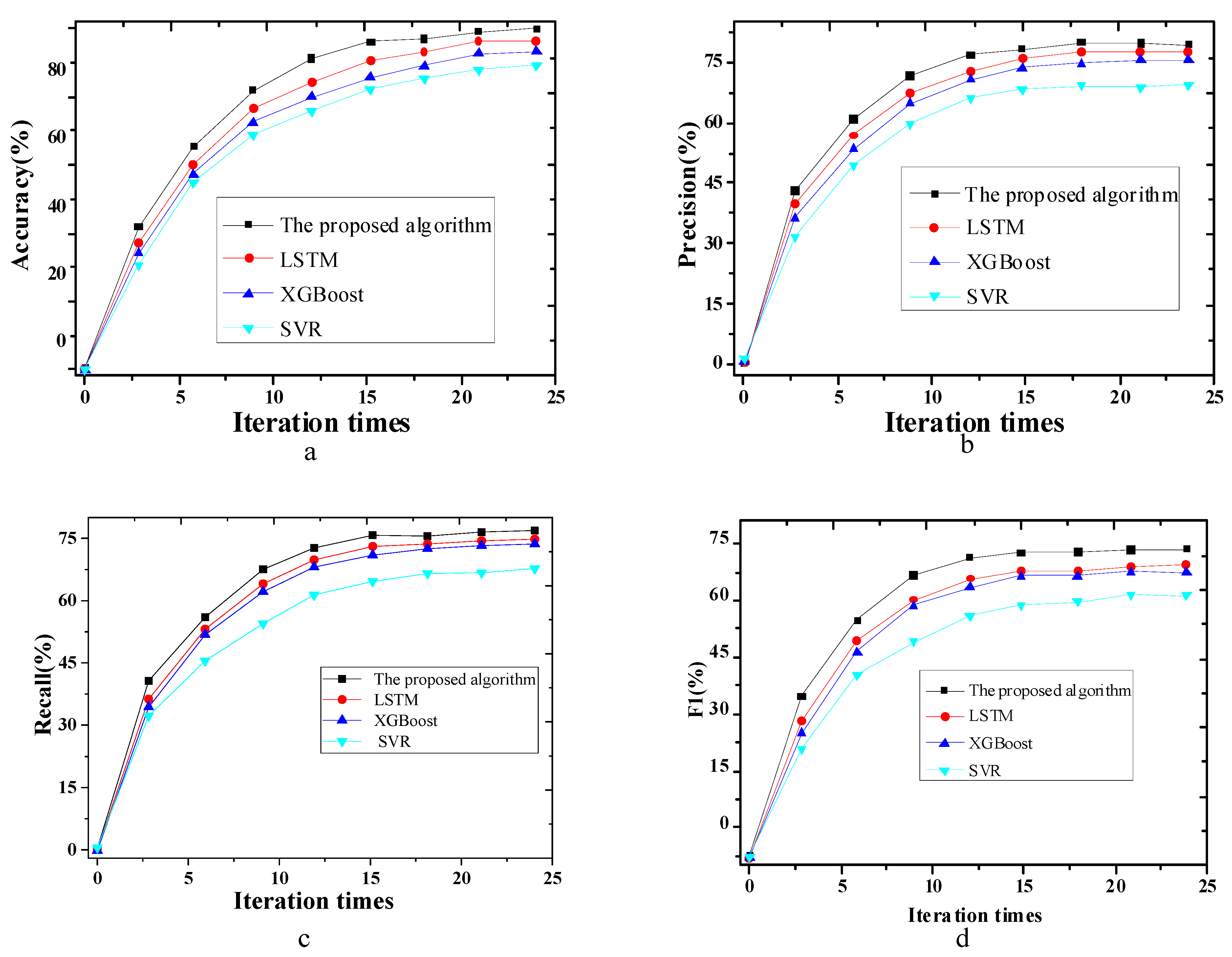
4.1. Comparative Analysis of the Fitting Effects of Self-Organizing LSTM Based on Sensitivity and Other Models

This section compares the proposed sensitivity-based self-organizing LSTM with LSTM, Extreme Gradient Boosting (XGBoost), and Support Vector Regression (SVR). Their performance is analyzed in terms of Accuracy, Precision, Recall, and F1-value. The results are unfolded in Figure 4:

Figure 4. Comparison of different algorithm performances ((a) accuracy; (b) precision; (c) recall; (d) F1-value).

In Figure 4, the proposed sensitivity-based self-organizing LSTM is compared with several classical models from the accuracy, precision, recall, and F1 perspectives. The experimental outcomes show that the accuracy of the proposed model is 89.24%, outperforming other classical algorithms. Accuracy is improved by at least 3.6%, which is 20% higher than the SVR model. At the same time, the proposed model has the highest precision, recall, and F1 values, over 2% higher than the control models. Compared with other classical algorithms, the sensitivity-based self-organizing LSTM algorithm has shown higher accuracy and minor error.

Figure 5 compares the prediction speed of different algorithms.

Figure 5. Model prediction speed test ((a) first test results; (b) second prediction results).

As per Figure 5, in the proposed sensitivity-based self-organizing LSTM, the response time corresponding to eight time points is distributed between 5.1 s and 5.9 s. The result suggests that the proposed model presents high real-time performance.

Table 2 compares the sensitivity-based self-organized LSTM algorithm with the LSTM, XGBoost, and SVR. In order to achieve this, the Root Mean Square Error (RMSE), Mean Absolute Error (MAE), Mean Absolute Percentage Error (MAPE), and R² of PM 2.5 concentrations are calculated at 7:00 a.m. at Stations A, B, and C.

Table 2. Performance comparison of PM 2.5 concentration estimation models in different Stations (A, B, and C).

	Different Models	RMSE μg.m−3	MAE μg.m−3	MAPE μg.m−3	R2
A (7:00, 0 m)	Self-organizing LSTM algorithm based on the sensitivity	120	115	132	0.826
	LSTM	110	111	110	0.833
	XGBoost	120	112	134	0.617
	SVR	112	145	101	0.842
	Calculated value	1.75	1.12	6.06	/
B (7:00, 0 m)	Self-organizing LSTM algorithm based on the sensitivity	110	120	115	0.859
	LSTM	111	121	123	0.86
	XGBoost	118	125	131	0.843
	SVR	120	125	132	0.790
	Calculated value	1.75	1.11	6.05	/
C (7:00, 0 m)	Self-organizing LSTM algorithm based on the sensitivity	118	115	112	0.867
	LSTM	110	123	145	0.777
	XGBoost	129	135	132	0.735
	SVR	134	132	130	0.805
	Calculated value	1.70	1.16	6.06	/

According to Table 2, the sensitivity-based self-organized LSTM PM 2.5 concentration estimation model proposed has a daily RMSE of 120 μg.m⁻³ at Station A. Apparently, the daily RMSE has decreased by 20.13%, 18.81%, and 29.51%, respectively, compared to LSTM, XGBoost, and SVR. On the other hand, with a daily MAE of 115 μg.m⁻³, the proposed self-organizing LSTM model’s MAE has decreased by 5.46%, 12.39%, and 7.09%, respectively, compared to LSTM, XGBoost, and SVR. The results show that the proposed sensitivity-based, self-organized LSTM PM 2.5 concentration estimation model can accurately predict PM 2.5 concentration in different regions. However, for Stations with low PM 2.5 concentration, the sensitivity-based self-organized LSTM PM 2.5 concentration estimation model’s prediction error is relatively large. The sensitivity-based self-organizing LSTM has RMSE, MAE, and MAPE of 1.75, 1.12, and 6.06, respectively, superior to LSTM, XGBoost, and SVR.

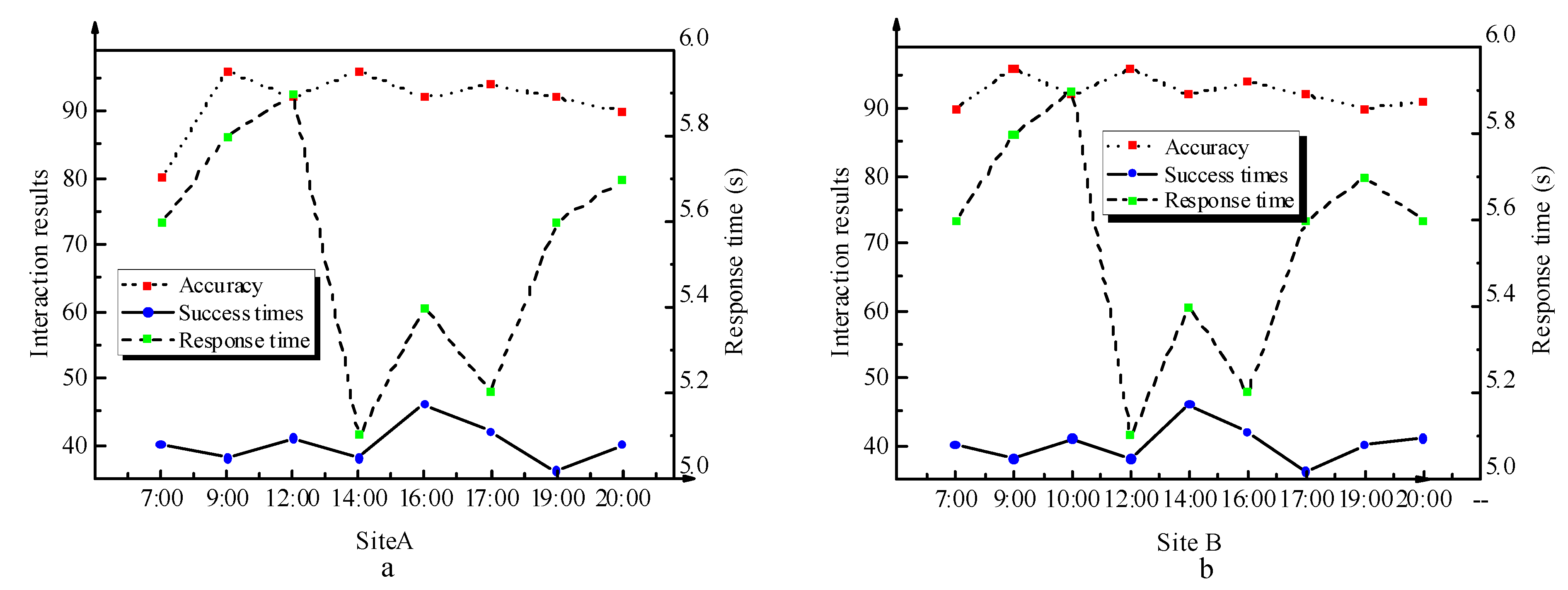
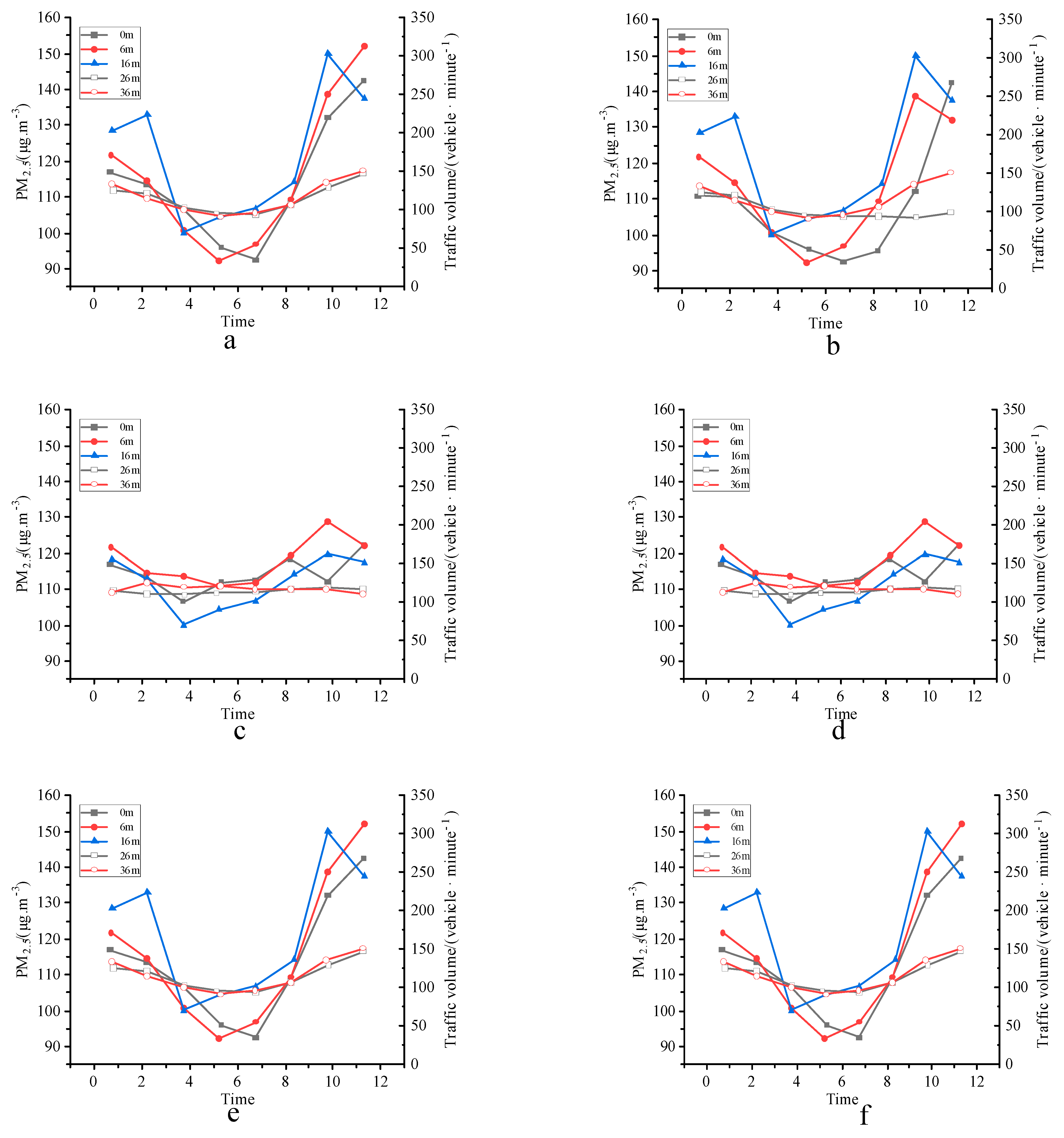
4.2. Comparison of Daily Changes in PM 2.5 Concentration

Figure 6 illustrates the diurnal PM 2.5 concentration variations at Stations A, B, and C before and after using the UGS planning scheme of the sensitivity-based self-organizing LSTM model proposed here.

Figure 6. Daily measure of PM 2.5 concentration ((a) Station A before UGS planning; (b) Station A after UGS planning; (c) Station B before UGS planning; (d) Sit B after UGS planning; (e) Station C before UGS planning; (f) Station C after UGS planning).

According to the daily measurement curve in Figure 6, before UGS planning near stations A, B, and C, the PM 2.5 concentration is low in the daytime but high at the beginning and the end of the day. Specifically, the PM 2.5 concentration of Stations A, B, and C’s nearby green belts increases from 8:00 a.m. to 10:00 p.m. It begins to decrease, reaching a minimum around 12:00–14:00. After that, PM 2.5 concentration rises until it reaches its maximum at 7:00 p.m. The urban traffic flow is closely related to the atmospheric PM 2.5 concentration difference.

After the UGS planning near Stations A, B, and C, the PM 2.5 concentration is also high in the morning and evening and low in the daytime. However, the variation range is relatively small. PM 2.5 concentration in the different green belts near stations A, B, and C has a slow trend of increasing from 9:00 a.m. The concentration begins to decline after 10:00 a.m., reaching a minimum value around 14:00. After that, PM 2.5 concentration slowly increases with the increase of traffic flow.

4.3. Experimental Results of the Reducing Effect of Road Greenbelt on PM 2.5

Table 3 lists the ability of green road space to reduce PM 2.5 under zero-pollution or light pollution conditions/moderate pollution conditions/severe pollution conditions.

Table 3. Experimental results of the reducing effect of road greenbelt on PM 2.5 at Stations A, B, and C.

Under Zero-Pollution or Light Pollution Conditions
Green Belt Width
6 m			16 m			26 m			36 m
A	B	C	A	B	C	A	B	C	A	B	C
7.24%	0.64%	0.5%	10.2%	1.46%	1.95%	9.31%	2.34%	4.52%	12.22%	3.54%	3.72%
Under Moderate Pollution Conditions
Green Belt Width
6 m			16 m			26 m			36 m
A	B	C	A	B	C	A	B	C	A	B	C
0.8%	−7.5%	−0.6%	3.4%	−4.2%	0.49%	0.83%	−2.6%	−2.5%	0.51%	−7.2%	−6.8%
Under Severe Pollution Conditions
Green Belt Width
6 m			16 m			26 m			36 m
A	B	C	A	B	C	A	B	C	A	B	C
−0.09%	−1.3%	−2.8%	−0.9%	−1.9%	−3.5%	−3.1%	−2.6%	−5.3%	−4.4%	−3.7%	−2.72%

Under zero-pollution or slightly polluting weather conditions throughout the year, the reduction function of green road space on PM 2.5 varies between different green belt widths and distances. On each measurement Station, there is a significant dust reduction function at a green belt width of 6 m, 16 m, 26 m, and 36 m. The green belt’s dust reduction rate order is C > A > B. Among the three green belts, the green belt near Station C has a higher reduction function on PM 2.5 than the other two green belts, with an average reduction rate of 9.70%. The highest reduction rate is at 36 m, reaching 12.22%. The order of reduction rates at different green belt widths is 36 m > 26 m > 16 m > 6 m. This is mainly because the dust reduction difference may be related to the configuration structure of green belts and plant species at various points. The composition of the green space community near Station C is mostly large trees, with a high canopy density in the forest, reaching 80%. Under moderately polluted weather conditions, the reduction function of green space on PM 2.5 is insignificant at different locations and greenbelt widths. Except for Station A’s green belt, the reduction rates of the other two green belts on PM 2.5 are primarily negative. The results indicate that certain weather pollution conditions restrict the effect of green space on PM 2.5 reduction. Furthermore, under the same weather conditions, different plant allocation modes significantly impact the PM 2.5 pollution in the air. For example, under severely polluted weather, or the PM 2.5 pollution reaches a level above severe, the reduction function of green road space on PM 2.5 in different locations and green belt widths is insignificant. At this time, the reduction function is negative. The findings corroborate that the UGS’s dust reduction and retention functions are limited. The dust reduction and retention functions are sometimes neglected, especially in highly polluted environments.

5. Conclusions

PM 2.5 is a tiny inhalable particulate with a radius of 1.25 or smaller in ambient air. Featuring small particle sizes and long transportation distances, PM 2.5 often contains complex harmful and even toxic substances. It does not easily settle down, causing air pollution and endangering public health and air quality. This work mainly studies prediction schemes based on LSTM and proposes an LSTM model based on the self-organizing algorithm. To this end, sensitivity is chosen as an indicator to increase or delete hidden layer neurons. This work determines the hidden layer neurons’ quantity after network training. From the experimental results, this determined quantity falls within the available range. Thereby, it ensures high prediction accuracy and alleviates difficulty in determining how many hidden layer neurons to choose. Further, the proposed sensitivity-based self-organizing LSTM algorithm is compared with LSTM, XGBoost, and SVR. The results show that the sensitivity-based self-organizing LSTM algorithm presents an RMSE, MAE, and MAPE of 1.75, 1.12, and 6.06, respectively, superior to LSTM, XGBoost, and SVR. Last but not least, there are still some shortcomings in the research results. The proposed model has certain areas for improvement in prediction accuracy. Therefore, the main direction of future work is expected to utilize or develop better deep learning models to improve the proposed model.

References

- Sultana, R.; Selim, S.A.; Alam, M.S. Diverse perceptions of supply and demand of cultural ecosystem services offered by urban green spaces in Dhaka, Bangladesh. J. Urban Ecol. 2022, 8, juac003. [Google Scholar] [CrossRef]
- Stessens, P.; Canters, F.; Huysmans, M.; Khan, A.Z. Urban green space qualities: An integrated approach towards GIS-based assessment reflecting user perception. Land Use Policy 2020, 91, 104319. [Google Scholar] [CrossRef]
- Geary, R.S.; Wheeler, B.; Lovell, R.; Jepson, R.; Hunter, R.; Rodgers, S. A call to action: Improving urban green spaces to reduce health inequalities exacerbated by COVID-19. Prev. Med. 2021, 145, 106425. [Google Scholar] [CrossRef]
- Wang, Z.; Deng, Y.; Zhou, S.; Wu, Z. Achieving sustainable development goal 9: A study of enterprise resource optimization based on artificial intelligence algorithms. Resour. Policy 2023, 80, 103212. [Google Scholar] [CrossRef]
- Yin, X. The Planning Strategy of Urban Space Under the Influence of Shared Transportation. Int. J. Soc. Sci. Educ. Res. 2020, 3, 84–87. [Google Scholar]
- Fialová, J.; Bamwesigye, D.; Łukaszkiewicz, J.; Fortuna-Antoszkiewicz, B. Smart Cities Landscape and Urban Planning for Sustainability in Brno City. Land 2021, 10, 870. [Google Scholar] [CrossRef]
- Zhang, J.; Yu, Z.; Zhao, B. Impact Mechanism of Urban Green Spaces in Promoting Public Health: Theoretical Framework and Inspiration for Practical Experiences. Landsc. Archit. Front. 2020, 8, 104–113. [Google Scholar] [CrossRef]
- Fialová, J.; Březina, D.; Žižlavská, N.; Michal, J.; Machar, I. Assessment of Visitor Preferences and Attendance to Singletrails in the Moravian Karst for the Sustainable Development Proposals. Sustainability 2019, 11, 3560. [Google Scholar] [CrossRef]
- Shan, J.; Huang, Z.; Chen, S.; Li, Y.; Ji, W. Green Space Planning and Landscape Sustainable Design in Smart Cities considering Public Green Space Demands of Different Formats. Complexity 2021, 2021, 5086636. [Google Scholar] [CrossRef]
- Lukaszewicz, J.; Fortuna-Antoszkiewicz, B.; Długoński, A.; Wiśniewski, P. From the heap to the park—Reclamation and adaptation of degraded urban areas for recreational functions in Poland. Sci. Rev. Eng. Environ. Sci. (SREES) 2019, 28, 664–681. [Google Scholar] [CrossRef]
- Wang, Z.; Liang, F.; Li, C.; Xiong, W.; Chen, Y.; Xie, F. Does China’s low-carbon city pilot policy promote green development? Evidence from the digital industry. J. Innov. Knowl. 2023, 8, 100339. [Google Scholar] [CrossRef]
- Hu, H.; Qi, S.; Chen, Y. Using green technology for a better tomorrow: How enterprises and government utilize the carbon trading system and incentive policies. China Econ. Rev. 2023, 78, 101933. [Google Scholar] [CrossRef]
- Zou, H.; Wang, X. Progress and Gaps in Research on Urban Green Space Morphology: A Review. Sustainability 2021, 13, 1202. [Google Scholar] [CrossRef]
- Łukaszkiewicz, J.; Fortuna-Antoszkiewicz, B.; Oleszczuk, Ł.; Fialová, J. The Potential of Tram Networks in the Revitalization of the Warsaw Landscape. Land 2021, 10, 375. [Google Scholar] [CrossRef]
- Liu, O.Y.; Russo, A. Assessing the contribution of urban green spaces in green infrastructure strategy planning for urban ecosystem conditions and services. Sustain. Cities Soc. 2021, 68, 102772. [Google Scholar] [CrossRef]
- Wang, A.; Wang, H.; Chan, E.H. The incompatibility in urban green space provision: An agent-based comparative study. J. Clean. Prod. 2020, 253, 120007. [Google Scholar] [CrossRef]
- Hu, H.; Xu, J.; Liu, M.; Lim, M.K. Vaccine supply chain management: An intelligent system utilizing blockchain, IoT and machine learning. J. Bus. Res. 2023, 156, 113480. [Google Scholar] [CrossRef]
- Suligowski, R.; Ciupa, T.; Cudny, W. Quantity assessment of urban green, blue, and grey spaces in Poland. Urban For. Urban Green. 2021, 64, 127276. [Google Scholar] [CrossRef]
- Wang, Z.; Zhang, S.; Zhao, Y.; Chen, C.; Dong, X. Risk prediction and credibility detection of network public opinion using blockchain technology. Technol. Forecast. Soc. Chang. 2023, 187, 122177. [Google Scholar] [CrossRef]
- Kim, M.; Rupprecht, C.D.; Furuya, K. Typology and Perception of Informal Green Space in Urban Interstices: A case study of Ichikawa City, Japan. Int. Rev. Spat. Plan. Sustain. Dev. 2020, 8, 4–20. [Google Scholar] [CrossRef]
- Ojeda-Revah, L.; González, Y.O.; Vera, L. Fragmented Urban Greenspace Planning in Major Mexican Municipalities. J. Urban Plan. Dev. 2020, 146, 04020019. [Google Scholar] [CrossRef]
- Xie, H.; Zhang, Y.; Chen, Y.; Peng, Q.; Liao, Z.; Zhu, J. A case study of development and utilization of urban underground space in Shenzhen and the Guangdong-Hong Kong-Macao Greater Bay Area. Tunn. Undergr. Space Technol. 2021, 107, 103651. [Google Scholar] [CrossRef]
- Hanson, H.I.; Eckberg, E.; Widenberg, M.; Olsson, J.A. Gardens’ contribution to people and urban green space. Urban For. Urban Green. 2021, 63, 127198. [Google Scholar] [CrossRef]
- Shekhar, S.; Aryal, J. Monitoring urban green spaces using geospatial technologies—A case study of Hobart, Tasmania, Australia. Trans. Inst. Indian Geogr. 2021, 43, 78–90. [Google Scholar]
- Cobbinah, P.B.; Asibey, M.O.; Zuneidu, M.A.; Erdiaw-Kwasie, M.O. Accommodating green spaces in cities: Perceptions and attitudes in slums. Cities 2021, 111, 103094. [Google Scholar] [CrossRef]
- Kuang, W.; Zhang, S.; Li, X.; Lu, D. A 30 m resolution dataset of China’s urban impervious surface area and green space, 2000–2018. Earth Syst. Sci. Data 2021, 13, 63–82. [Google Scholar] [CrossRef]
- Li, C.; Xu, Y.; Zheng, H.; Wang, Z.; Han, H.; Zeng, L. Artificial intelligence, resource reallocation, and corporate innovation efficiency: Evidence from China’s listed companies. Resour. Policy 2023, 81, 103324. [Google Scholar] [CrossRef]
- Sari, D.A.K.; Widyawati, L.F.; Pramesti, D. The availability and role of urban green space in South Jakarta. IOP Conf. Ser. Earth Environ. Sci. 2020, 447, 012055. [Google Scholar] [CrossRef]
- Cobbinah, P.B.; Nyame, V. A city on the edge: The political ecology of urban green space. Environ. Urban. 2021, 33, 413–435. [Google Scholar] [CrossRef]
- Ghosh, S.; Das Chatterjee, N.; Dinda, S. Urban ecological security assessment and forecasting using integrated DEMATEL-ANP and CA-Markov models: A case study on Kolkata Metropolitan Area, India. Sustain. Cities Soc. 2021, 68, 102773. [Google Scholar] [CrossRef]
- Tamara, M.E.L.; Latty, T.; Threlfall, C.G.; Hochuli, D.F. Major insect groups show distinct responses to local and regional attributes of urban green spaces. Landsc. Urban Plan. 2021, 216, 104238. [Google Scholar] [CrossRef]
- Vaňo, S.; Olafsson, A.S.; Mederly, P. Advancing urban green infrastructure through participatory integrated planning: A case from Slovakia. Urban For. Urban Green. 2021, 58, 126957. [Google Scholar] [CrossRef]
- Guo, J.; Niu, H.; Xiao, D.; Sun, X.; Fan, L. Urban Green-space Water-consumption characteristics and its driving factors in China. Ecol. Indic. 2021, 130, 108076. [Google Scholar] [CrossRef]
- Huera-Lucero, T.; Salas-Ruiz, A.; Changoluisa, D.; Bravo-Medina, C. Towards Sustainable Urban Planning for Puyo (Ecuador): Amazon Forest Landscape as Potential Green Infrastructure. Sustainability 2020, 12, 4768. [Google Scholar] [CrossRef]
- Kim, D.; Ho, C.-H.; Park, I.; Kim, J.; Chang, L.-S.; Choi, M.-H. Untangling the contribution of input parameters to an artificial intelligence PM2.5 forecast model using the layer-wise relevance propagation method. Atmos. Environ. 2022, 276, 119034. [Google Scholar] [CrossRef]
- Cho, S.; Park, H.; Son, J.; Chang, L. Development of the Global to Mesoscale Air Quality Forecast and Analysis System (GMAF) and Its Application to PM2.5 Forecast in Korea. Atmosphere 2021, 12, 411. [Google Scholar] [CrossRef]
- Lu, G.; Yu, E.; Wang, Y.; Li, H.; Cheng, D.; Huang, L.; Liu, Z.; Manomaiphiboon, K.; Li, L. A Novel Hybrid Machine Learning Method (OR-ELM-AR) Used in Forecast of PM2.5 Concentrations and Its Forecast Performance Evaluation. Atmosphere 2021, 12, 78. [Google Scholar] [CrossRef]
- Rybak, A.; Rybak, A. The Impact of the COVID-19 Pandemic on Gaseous and Solid Air Pollutants Concentrations and Emissions in the EU, with Particular Emphasis on Poland. Energies 2021, 14, 3264. [Google Scholar] [CrossRef]
- Hu, H.; Xie, N.; Fang, D.; Zhang, X. The role of renewable energy consumption and commercial services trade in carbon dioxide reduction: Evidence from 25 developing countries. Appl. Energy 2018, 211, 1229–1244. [Google Scholar] [CrossRef]
Disclaimer/Publisher’s Note: The statements, opinions and data contained in all publications are solely those of the individual author(s) and contributor(s) and not of MDPI and/or the editor(s). MDPI and/or the editor(s) disclaim responsibility for any injury to people or property resulting from any ideas, methods, instructions or products referred to in the content. |
© 2023 by the authors. Licensee MDPI, Basel, Switzerland. This article is an open access article distributed under the terms and conditions of the Creative Commons Attribution (CC BY) license (https://creativecommons.org/licenses/by/4.0/).