Integrated Thermodynamic and Control Modeling of an Air-to-Water Heat Pump for Estimating Energy-Saving Potential and Flexibility in the Building Sector

Abstract

Reversible heat pumps are increasingly adopted for meeting the demand for space heating and cooling in buildings. These technologies will play a key role not only in the decarbonization of space air conditioning but also in the development of 100% renewable energy systems. However, to assess the achievable benefits through the adoption of these technologies in novel applications, reliable models are needed, capable of simulating both their steady-state operation and dynamic response at different conditions in terms of heating loads, outdoor temperatures, and so on. The operation of heat pumps is often investigated by highly simplified models, using performance data drawn from catalogs and paying scarce attention to the critical influence of controllers. In this respect, this paper proposed an integrated thermodynamic and control modeling for a reversible air-to-water heat pump. The study considered a heat pump alternatively equipped with variable-speed compressors and constant-speed compressors with sequential control. The developed modeling was then used to investigate the operation of an air-to-water heat pump serving an office building in Italy. Results show that the model provided insights into the transient operation of variable-speed heat pumps (e.g., the settling time). Regarding constant-speed heat pumps, the model provided hints of interest to the control engineer to prevent, in the examined case study, the risk of quick compressors cycling on low-load heating days or when low-temperature heating devices are supplied. Finally, using a control strategy based on a heating curve for the variable-speed heat pump, results show the potential for a sensible increase in the average coefficient of performance, from 17% up to 50%.

1. Introduction

In 2021, space and water heating accounted for nearly half of the energy demand of buildings [1]. The covering of this demand contributed, in its turn, to 80% of the carbon dioxide emissions of this sector. To achieve decarbonization of space and water heating, in the last two decades, a gradual shift from gas boilers to heat pumps (HP) was observed [2]. In this regard, according to recent statistics [3], the number of HPs sold and stored annually in European Union (EU) countries increased almost exponentially since 2005. In addition, the EU Commission recently emphasized the urgent need to deploy HPs as a strategy to address climate change and the energy crisis [4].

HPs are currently considered key technologies not only for decarbonizing the heating sector but also for the achievement of 100% renewable energy systems [5,6,7]. In this respect, they could provide ancillary services to the power grid, thus allowing for the integration of renewable energy sources (RES) [8,9]. In particular, through demand response (DR) programs [10], HPs will be activated (or modulated and deactivated) in case of electricity surplus (or deficit) from RES, with the thermal energy produced directly consumed or stored in ad hoc systems [11,12]. Regarding the latter option, in the case of the connection of buildings to low-temperature heating networks, the heat produced onsite by the HPs could be sold to the grid, and buildings could, thus, contribute to a more sustainable heat generation [13]. Looking at the building scale, the adoption of HPs along with thermal storage contributes to increasing the so-called “flexibility”, which is the capability of the building to modify its demand to meet external requests from the grid while assuring occupants’ comfort [14,15,16,17]. Several studies were conducted to highlight the benefits and drawbacks of these innovative applications of HPs. In particular, to improve the performance of HPs in buildings, large efforts were devoted by research to (i) improving the HP modeling to better predict the coefficient of performance (COP), and (ii) proposing innovative control strategies aimed at optimizing either COP or improving buildings’ flexibility.

Concerning HP modeling, in recent years, some authors proposed different ways to accurately describe the HP behavior. For instance, Zanetti et al. [18] carried out an experimental investigation of an air/ground reversible dual source HP, while developing an accurate model for predicting the COP. Puttige et al. [19] developed models of HPs using an artificial neural network based on data available from many field measurements. With some refinements to the model, the accuracy was improved with a relative root mean square error of less than 5%. In another paper, Puttige et al. [20] developed a modeling of ground-source HP by jointly using physical modeling and an artificial neural network to describe the long-term behavior of the ground. The model accuracy was duly checked by considering real data collected during the four years operation of a real system. Maier et al. [21] evaluated the effect of HP modeling in the context of model predictive control techniques. The authors found that a quadratic model offers the best compromise between computational efforts and accuracy. Liu and Cai [22] proposed a methodology to develop gray-box modeling for variable-speed HP in the case of limited training data. Artuso et al. [23] modeled a reversible HP using carbon dioxide as a refrigerant. Validation of the proposed modeling showed that the accuracy was higher in heating mode than in cooling mode. Xu et al. [24] relied on an artificial neural network for estimating cycling losses on constant speed HP. Kim et al. [25] developed a dynamic model of a variable-speed HP by using transfer functions to be included in the analysis of strategy for supporting power grid operators in frequency regulation. Abid et al. [26] developed a model of a domestic reversible variable-speed HP based on ad hoc experiments. The developed modeling was then used to determine optimal operating conditions. Zakula et al. [27] developed a thermodynamic model of a variable-speed HP operating in cooling mode while considering pressure drops, refrigerant back leakage, and variations in heat transfer coefficients. The comparison of simulation results to experimental data showed errors of less than ±10%. Other studies focused on modeling the HPs’ behavior including the frosting and defrosting processes to achieve a more realistic assessment of the seasonal COP. For instance, Ma et al. [28] developed a dynamic model of air-source HPs to account for frosting and reverse-cycle defrosting. The comparison of simulation results against experimental data proved the capability to describe the cycling operation due to frosting and defrosting. Roccatello et al. [29] developed correlations to account for the reduction in the HP performance due to startup and defrosting cycles. The results found, using the validated model, showed that these phases could lead to a 15% degradation of the performance from the value observed in steady-state operation. Rossi di Schio et al. [30] included the defrosting cycles in HP modeling for dynamic simulations in the TRNSYS environment. Sezen and Gunfor [31] developed a mathematical model for an air-source HP to account for the variation of performance with outdoor temperature and relative humidity. Popovac et al. [32] solved the frosting model for air-source HP in an OpenFOAM environment. Bagarella et al. [33] performed an energy analysis of the operation of both variable speed and ON–OFF HPs serving a single-family house, by considering the effect of storage sizing and the cycling losses. Liu et al. [34] developed and validated the modeling of an air-source HP which accounts for frosting and de-frosting. The modeling was then used to determine the operating conditions which could help limit frost formation. Rasmussen et al. [35] developed a detailed state-space modeling of the HP to test the capability of this technology in contributing to primary frequency regulation.

Regarding studies on innovative HPs operating strategies, most of the published studies proposed sophisticated controls by relying on model-based or rule-based methods. For instance, Bechtel et al. [36] used model predictive control to optimize HP operation while considering variable electricity prices. Ding et al. [37] proposed an optimization approach to operating the HPs and the heating system for an office building in case of DR provision including building load uncertainty by using a quantile regression neural network. The results showed a 35.8% reduction in operating costs compared with the conventional operating strategy. Abookersh et al. [38] compared two control strategies for the flexible operation of HPs coupled to seasonal storage in a low-temperature district heating network. Montrose et al. [39] proposed an optimal control algorithm, which aimed at minimizing the overall power consumption of variable-speed HPs by regulating the indoor temperature setpoint through peer-to-peer communication. Lee et al. [40] proposed an operation strategy for variable-speed HP based on mixed-integer model predictive control. The model allowed not only to prevent the operation of the HP with lots of compressor cycling but also to predict future heat load and ambient air temperatures. The results showed a maximum 22% reduction in electricity cost and carbon emissions. Dengiz et al. [41] proposed a heuristic control for the flexible operation of HPs coupled with a photovoltaic supplying underfloor heating system and a domestic hot water tank. The authors found a maximum 13.3% reduction in operating cost compared to a conventional control strategy and a 52.6% reduction in the surplus of energy produced onsite. Maier et al. [21] found that HP management through model predictive control outperformed operating strategies based on heating curves. Baeten et al. [42] proposed a multi-objective model predictive control for residential HPs for promoting flexible operation. The results indicated the capability of the controller to shift peak load. However, the authors stressed that in the case of DR needs, HP owners should be encouraged to participate by remunerating them for their additional expenses. Efkarpidis et al. [43] proposed an optimization method to operate HPs along with solar thermal collectors, batteries, and thermal energy storage aiming at maximizing self-consumption. Arteconi and Polonara [44] developed an HP control based on electricity price which varied HP’s temperature set point based on the variation of electricity market price. The study revealed that a substantial decrease in peak demand could be achieved. Schibuola et al. [45] compared operating strategies for DR for an HP-coupled photovoltaic system. Other studies investigated the capability of HPs in supporting transmission and system operators by providing ancillary services. Meesenburg et al. [46] found that large two-stage ammonia HPs can provide ancillary services thanks to their capability to quickly vary the electrical energy consumed. More specifically, the authors estimated that the HP’s power input could be varied by about 50% in 85 s while maintaining a safe compressor’s operation. Regarding HPs in the residential sector, Manner et al. [47] found that the aggregation of residential HPs could guarantee valid support for ancillary services. However, the authors stressed the importance to develop a real-time control system to manage the whole aggregated system. Rodriguez et al. [48] developed and validated a model for managing a cluster of residential HPs in the case of frequency regulation. The model revealed that the DR potential of aggregated HPs is significant, but particular attention needs to be given to the number of activation times of HPs and, most importantly, to the duration. Bartolucci et al. [49] showed that worthy cost savings could be achieved by the provision of ancillary services via large HPs coupled with thermal storage.

The previous literature review showed a strong research interest in the modeling of HPs behavior (as demonstrated by the large use of machine learning techniques or from research on frost buildup and removal) or improving performance during operation by advanced supervisory controllers. However, regardless of the purposes, integrated thermodynamic and control modeling was never performed. More specifically, regarding thermodynamic modeling, the performance variation due to time-changing boundary conditions (e.g., the outdoor temperature) or the part-load operation is typically estimated using catalogs’ data corrected by empirical factors [14,16]. In addition, the control strategy adopted to meet the user’s heating demand (and then the dynamic response) is not accounted for [43,50]. Finally, other studies focused on the development of refined HPs’ control strategies for the provision of DR but using very simplified thermodynamic modeling [16,21,45]. Considering the novel applications of HPs, it is of paramount importance to rely on a detailed thermodynamic and control model. In this respect, some papers pointed out that issues could arise when HPs are used to provide flexibility, which cannot be detected by relying on very simplified models. For instance, Liu et al. [51] pointed out that drastic changes in the compressor speed due to load balancing can lead to wet compression and then to compressor damage. Clauß and Georges [52] underlined that in short-time operation, the transient effects of the HP, such as cycling losses during start-up, are important. Bagarella et al. [53] found via experiments that cycling losses due to ON–OFF control could reduce the performance by up to 13% compared to a steady-state operation.

To fill the previous gap, this paper proposes a modeling of a reversible air-to-water HP where the thermodynamic aspects are jointly solved with the embedded control architecture. More specifically, the analysis will address the capability of the integrated modeling to provide insights into the dynamic response of the HP such as the time needed to reach new steady–steady operation, overshoot of supply water temperature after load change, number of compressors cycling per hour, etc., which are useful in the framework of novel applications of this technology. To show these capabilities, this study investigated:

-

The dynamic response of HP for the two typical compressor management strategies: (i) a sequential control of multiple compressors, with compressors running at a constant speed, and (ii) a variable-speed control where the rotating speed of the compressors is continuously varied;

-

The capability to analyze new HPs’ management strategies aimed at increasing the seasonal COP or improving building flexibility. In this respect, this paper investigated the typical control of the HPs based on “heating curves” which assumes a variable temperature setpoint of the hot water with the outdoor temperature;

-

The analysis of the dynamic operation of the HP when comparing different heating devices supplied by HPs (e.g., fan coils or heating floor).

A reversible air-to-water HP serving an office located in Southern Italy was assumed as the case study. Some scenarios will be simulated to account for the control strategies adopted and some safety issues on compressor operations (i.e., the number of “ON–OFF” cycles). Before ending, some details on the structure of this paper are due. In the Section 2, both the thermodynamic and control modeling are described. In the Section 3, the case study is presented together with the performed simulation. In the Section 4, results are shown and discussed, while in the Section 5, some conclusions are drawn.

2. Materials and Methods

Before providing details on the thermodynamic and control modeling of a reversible air-to-water HP, a schematic description of the reference unit is due. Figure 1 shows the components along with the main variables and acronyms. The refrigerant flow is indicated by the red arrows for the “heating mode” and the blue arrows for the “cooling mode”. An air-to-refrigerant heat exchanger (e.g., a tube and fins coil or plate and fins) is used as the condenser (CND) during the summer, and as the evaporator (EVP) during the winter. It is worth noting that the temperature and relative humidity of the outdoor air is indicated as ODT and RH, respectively. A brazed-plate heat exchanger is used to cool or heat the water coming from the hydraulic loop. The temperature of the water returning from the hydronic loop is indicated as T_wr. Then, the HP heats (or cools down) the water flow rate to a desired temperature, indicated here as “supply temperature”, T_ws (green arrow in the figure). As shown in the figure, the compressor (CMP) is typically driven by an induction motor (IM). To maintain a desired value of the temperature of T_ws, the controller (CTRL) will act on the IM by regulating the speed (in the case of variable speed drive) or cycling it “ON” and “OFF” (in the case of constant speed CMPs).

2.1. Thermodynamic Modeling of an Air-to-Water Heat Pump Operating in Heating Mode

Equation (1a,b) show the main variables which affect the delivered heating capacity (HC) and the required mechanical power ($P_{m,H}$) for an air-to-water HP. More specifically, both quantities were dependent on the compressor rotating speed (${\omega }_{CMP}$), the dry-bulb temperature, and the relative humidity of the outdoor air (indicated as $ODT$ and $RH$, respectively), and the temperature of the water returning from the building and entering the HP’s CND ($T_{wr}$).

$$HC=f\left(ODT,RH,{\omega }_{CMP},T_{wr}\right)$$

(1a)

$$P_{m,H}=g\left(ODT,RH,{\omega }_{CMP},T_{wr}\right)$$

(1b)

In this work, Equation (2a,b) were used for representing Equation (1a,b). More specifically, as shown in the cited equations, HC and $P_{m,H}$ are given as a linear function of the main variables,

$$HC=L_1{\omega }_{CMP}+L_{2}ODT+L_3{T}_{wr}$$

(2a)

$$P_{m,H}=K_1{\omega }_{CMP}+K_{2}ODT+K_3{T}_{wr}$$

(2b)

where $K_1,L_1$,$L_2$, $K_2$, $L_3$, and $K_3$, are fitting coefficients for ${\omega }_{CMP}$, $ODT$, and $T_{wr}$. These unknown coefficients can be derived by using numerical methods applied to data collected from experiments or ad hoc simulations. It is worth noting that, unlike Equation (1a,b), RH is not included in Equation (2a,b). As will be seen later, the moderately cold winter of the reference climatic zone did not result in frost formation on the evaporator surface. Therefore, the RH value had a negligible influence in this case. In this respect, it is also necessary to stress that the model described in the following was limited only to those cases where the defrosting cycle was rarely activated.

Regarding the ODT values in Equation (2a,b), they can be obtained by using a weather database. Conversely, the temperature of the water returning from the hydraulic loop, i.e., $T_{wr}$, depends on the heating demand of the user (in the following indicated as heating load, HL) and the thermal inertia of the hydronic loop. More specifically, Equation (3) represents the dynamic model of the hydronic circuit served by the HP,

$$\frac{d{T}_{wr}}{dt}=\frac{1}{C_s}(HC-HL)$$

(3)

where the variation of $T_{wr}$ is directly related to the difference between HC and HL (i.e., the difference between the HP’s capacity and the heating load). $C_s$ is a coefficient (kJ/°C) used to account for the inertia of the hydronic loop coupled to the HP. Equation (4a,b) were adopted to estimate this quantity. More specifically, in Equation (4a), ρ_w is the density of water, c_w is the specific heat capacity of water, and V_des is the desired volume of water in the hydronic loop. This quantity was derived from “Portoso’s Equation” [54], and it is often adopted as a “rule of thumb” to estimate the desired amount of water in the hydronic loop, needed for the safe operation of the CMPs,

$$C_s={\mathsf{\rho }}_w{c}_w{V}_{des}$$

(4a)

$$V_{des}=\frac{60C_{nom}}{{\mathsf{\rho }}_w{c}_w{\left(\frac{∆T}{∆\tau }\right)}_{ref}}$$

(4b)

In Equation (4b), C_nom is the nominal capacity delivered by the HP (typically in cooling mode) at the design condition and ${\left(\frac{∆T}{∆\tau }\right)}_{ref}$ is the maximum variation of the water return temperature from the hydronic loop (typically set to 5 °C/min).

Finally, the temperature of the water supplied to the building ($T_{ws})$ is calculated by applying the energy conservation equation to the HP as shown in Equation (5),

$$T_{ws}=T_{wr}+\frac{HC}{{\dot{m}}_w{c}_w}$$

(5)

where ${\dot{m}}_w$ is the mass flow rate of water circulating entering the HP. Note that $T_{ws}$ is assumed as the controlled variable by the action of the controller.

2.2. Description and Modeling of the Control Strategies

The heating/cooling capacity delivered by air-to-water HPs can be varied in two ways: (i) by using variable-speed drives (VFD) coupled to IMs which continuously change the CMP’s rotating speed ${\omega }_{CMP}$ to meet the desired “supply water temperature setpoint (T_ws,ref)”; (ii) cycling ON–OFF constant-speed CMPs to maintain the supply water temperature around a desired value.

2.2.1. Details on the Control Scheme for the Variable-Speed HP

Figure 2 depicts the main components of the control scheme for the case of variable-speed HPs. The CMP rotating speed (which is an output of the IM) was modulated thanks to the action of VFD. More specifically, a scaler control was used inside the VFD, where a simple “voltage over frequency V/F” technique was used to control an IM at variable speed. More insights into the scaler control are provided in [55].

A proportional and integral (PI) temperature controller provides the reference value of the speed to the V/F control (i.e., ω_ref). Such a value is quantified based on the difference between the measured supply water temperature and the desired value (i.e., ΔT_ws). Then, as shown in the figure, the V/F control gives as output the duty cycles, D_a,b,c to the voltage source inverter (VSI). In this component, then, space vector modulation (SVM) is used to acquire the duty cycles, and the three-phase voltage V_a,b,c are provided by the VSI to the IM [55].

In the “Heat Pump” block, HP’s thermodynamic model (i.e., Equation (2a,b)) was implemented.

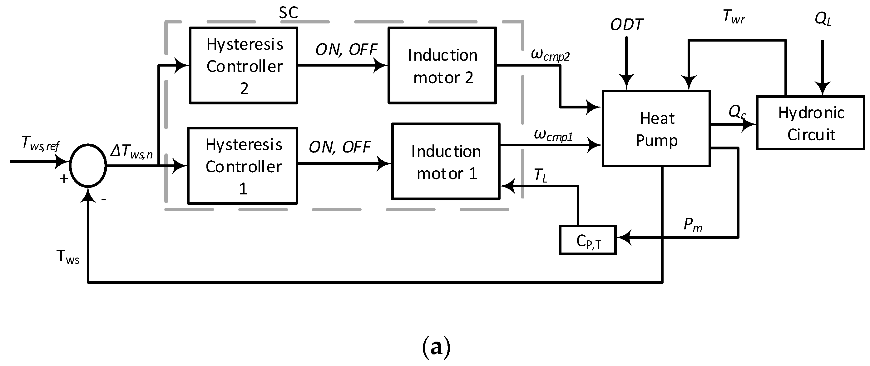
2.2.2. Details on the Control Scheme for HPs with Constant-Speed Compressors

Figure 3a shows the scheme for the control of a constant speed HP equipped with multiple CMPs. More specifically, CMPs were “sequentially” activated or deactivated based on the difference between the measured water supply temperature and the desired value ${∆T}_{ws,n}=T_{ws}-T_{ws,ref}$. To better understand the sequential control logic (SC), it is worth referring to Figure 3b. This figure depicts an SC in the case of an HP with two CMPs. The black line represents the time evolution of the measured value of the hot water supply temperature. The horizontal red lines indicated by $T_{ws}\pm {∆T}_{ws,n}$ values represent the temperature threshold values for cycling “ON” and “OFF” each CMP. It was apparent that the narrow band for $\pm {∆T}_{ws,n}$ could lead to many cycles of each CMPs. Conversely, a large band could be responsible for high T_ws variation, thus leading to occupants’ discomfort. The values of $\pm {∆T}_{ws,n}$ are typically selected to assure a maximum number of ON–OFF cycles in an hour below the limit recommended for CMP safety. As shown in Figure 3a, a hysteresis controller can be used for solving the ON–OFF cycle of each CMP.

3. Case Study: Description and Simulation

To investigate the capability of the proposed model in describing the dynamic response of an air-to-water HP coupled with a hydronic circuit, an office building was selected as a case study. The reference building was located in Palermo (Italy). In Figure 4a, the hourly profiles for ODT are shown for two typical weekdays in winter. One was characterized by a high heating load due to the low ODT (i.e., around the beginning of February) and the other one by a low heating load (i.e., around the half of April). It is worth noting that in Figure 4a,b, the dashed line is used for the profile on the low heating day and the continuous line for the high load day. Heating demand profiles (Figure 4b) were estimated using data from a previous study performed by one of the authors [56]. Conversely, the daily profiles of ODT (on an hourly basis) are retrieved using the meteorological dataset [57]. Looking at Figure 4a,b, it was assumed to be a 10 h per day operation (more specifically, from 7 AM to 5 PM) with load variations at a 15 min time step. Note that the minimum demand was observed between 12 PM and 2 PM (when higher ODT values were observed).

3.1. Details on the Air-to-Water Heat Pump

As previously mentioned, an air-to-water HP was here assumed as the reference system. However, the selection of the nominal HP capacity was based on the peak of cooling demand. This approach is simply explained by considering that for the assumed locality, cooling demand was prevalent compared to the heating one due to the moderately cold winter and the very hot summer. For this reason, based on the 49 kW_c peak in the cooling demand, a reversible HP with a 50 kW_c cooling capacity was selected. The corresponding delivered HC (in the design condition) results to be around 62 kW_th.

Table 1. Matrix test for the HP thermodynamic modeling.

Refrigerant Circuit
Refrigerant	R410a
Condenser Type	Fin and Tube
Number of Condenser	1
Condenser Fan Power [kW]	1.5
Metering Device	Electronic Expansion Valve (EEV)
Evaporator Water Flowrate [m3/h]	7.0
Evaporator Pump Power [kW]	2
Compressor Type (and Number)	Scroll (no. 2)
Compressor Power (each) [kW]	9.0
Refrigerant Charge [kg]	14.3

summarized the main technical features of the selected HP. These data were derived from commercial catalogs.

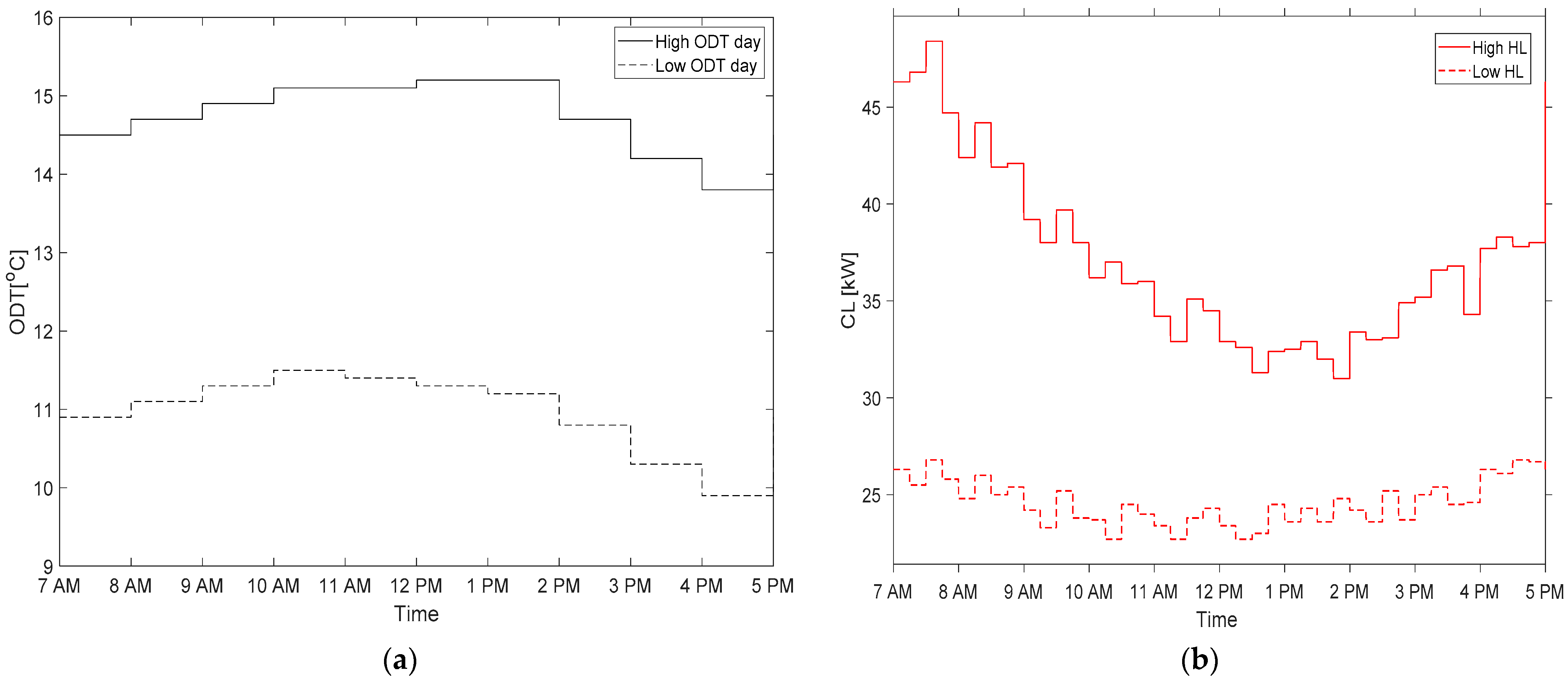
3.2. Details on Simulation Performed and Assumptions

The assumed air-to-water HP was equipped with two scroll compressors (Table 1). In this respect, the following strategies CMPs’ operation were here investigated:

-

Variable-speed CMPs, where the speed of both CMPs is continuously varied between minimum and maximum values via VFDs, as shown in Figure 2 (in the following, this option will be briefly indicated as variable-speed HP);

-

Constant-speed CMPs with sequential control, where, since the CMPs speed is constant, the heating demand is covered by cycling ON–OFF each CMPs following a sequential approach, as shown in Figure 3a (this option will be briefly indicated as constant-speed HP).

The thermodynamic modeling of the HP of the considered HP was developed via IMST-Art v.4.0 software [58]. More specifically, the software allowed for 1-D modeling of heat exchangers, and other accessories, and the reliability of results was confirmed by ad hoc validation studies [59].

Table 2. Matrix test for the HP thermodynamic modeling.

Variable		Range	Interval	HP Control
ODT	[°C]	5–17	+4 °C	Variable-Speed CMPs
				ωCMP [rpm]
				1000–6200	(+400 rpm)
Tw,r	[°C]	25–55	+10 °C	ON-OFF CMPs
				ωCMP [rpm]
				2900	(-)

summarizes the boundary conditions selected to characterize the HP operation via simulations. Regarding the ODT, its value varied from 5 to 17 °C, to account for the time variation of ODT during the day and the season. More specifically, a 4 °C step variation was assumed, leading to four values to be simulated. Regarding the temperature of the water returning from the building, T_wr, and entering the HP, the range 25–55 °C was selected to account for different heating/cooling demands (which leads, in turn, to part-load operation of the HP) or supplied heating devices (e.g., fan coils or heating floors). A 10 °C step variation was assumed as well, again resulting in four T_wr values to be simulated.

For variable-speed CMPs, a survey on commercially available scroll CMPs for HPs highlights that the rotating speed ω_CMP typically varied between 1000 and 6200 rpm, thanks to a large set of frequencies provided by the VFD. Then, the matrix test in Table 2 shows that the rotating speed of each compressor was varied between 1000 and 6200 rpm, with a 400 rpm step variation which leads to fourteen ω_CMP values to be simulated. The number of simulation tests to be performed to characterize the variable-speed HP’s thermodynamic modeling was then obtained by combining four ODT, four T_wr values, and fourteen compressor speeds.

In the case of constant-speed CMPs, conversely, commercial catalogs indicated a nominal rotating speed equal to 2900 rpm. By combining the four ODT values, and the four T_wr values, simulations were first carried out with only one CMP “ON”. Then, tests were performed again considering both CMPs “ON”.

To calculate the K_i and L_i fitting coefficients in Equation (2a,b), the least square method (LS) was applied to data from the simulations. This analysis was performed in MATLAB software R2022b. The results are presented in

Table 3. Preliminary modeling results: variable-speed HP.

	Delivered Capacity			Absorbed Power
VS-Heating	L1	0.012	RMSE [kW]: 3.01 NRMSE [%]: 3.34	K1	0.0034	RMSE [kW]: 1.71 NRMSE [%]: 7.15
	L2	1.21		K2	−0.083
	L3	−0.21		K3	0.089

and

Table 4. Preliminary modeling results: constant-speed HP with two CMPs “ON”.

	Delivered Capacity			Absorbed Power
CS-Heating	L1	0.0107	RMSE [kW]: 0.704 NRMSE [%]: 3.66	K1	0.0004	RMSE [kW]: 0.102 NRMSE [%]: 1.87
	L2	0.9572		K2	−0.0002
	L3	−0.207		K3	0.1698

. As shown, the normalized root mean square error index (NRMSE) was used to quantify the error of the model to the thermodynamic data. As shown in Table 3 and Table 4, the NRMSE always resulted lower than 7.5%, which can be considered a good approximation for the scope of the analysis.

3.3. Implementation of a Control Strategy Based on the “Heating Curve”

According to the declared goals of this work, the developed model was supposed to enable an assessment of the benefits that could be achieved when operating the HP with a variable water supply temperature, T_ws,ref, instead of a constant temperature. The use of a water supply temperature to the building variable with the ODT is typical in both HPs and gas boilers. In this respect, the possibility for the HP to operate with lower condensing pressures during “moderately” cold periods could lead to lower energy consumption and significantly higher COP values. In addition, the use of variable temperature setpoint was identified as a strategy for implementing DR programs in the building sector via HPs [44]. The variation of T_ws,ref with ODT is usually presented in the form of a so-called “heating curve”. These curves are supplied by manufacturers in catalogs and embedded in the HPs’ control.

Before developing a heating curve for the considered HP, a preliminary assessment of the effects of a reduction in the hot water supply temperature on the sensible heating capacity of the fan coil was performed. This analysis relied on the model implemented in TRNSYS v. 17 [60] through Type 600a and validated, in the framework of this work, using data from different fan coil manufacturers [61]. Figure 5a plots the fan coil’s sensible capacity vs. the hot water temperature supplied. As shown, the T_ws varied in the range of 35.0–50.0 °C. Note that when the temperature of the supplied water decreased from 50 °C to 35 °C, about a 50% reduction in the heating capacity of the fan coil was observed. Although a heavy reduction in fan coil capacity was consequent, the assumption of a variable supply water temperature of hot water over the 35.0–50.0 °C range with increasing ODT sounds reasonable. Indeed, in the case of higher ODT values, a reduction in the user’s heating demand was expected due to lower heat loss from the indoor to the outdoor environment. Then, the fan coils should satisfy a lower demand. In Figure 5b, a heating curve of the HP is shown. A linear change in T_ws,ref vs. ODT was assumed. In particular, a T_ws,ref was always maintained at 50 °C for ODT values lower than 30 °C. A linear decrease down to 35 °C was assumed as ODT gradually increased up to 15 °C; for ODT value greater than 15 °C, T_ws,ref was equal to 35 °C. Before concluding, it is worth stressing that, for the sake of brevity, this strategy will be applied only for the variable-speed HP.

3.4. Details on Model Solving and Main Assumptions

The control architectures for both variable- and constant-speed HPs were solved by using MATLAB Simulink. The simulations were performed for the full-day operation (i.e., for 10 h) and a sample time equal to 0.01 s was used to reduce computational efforts.

The variable-speed HP was controlled by assuming for the supply water temperature a 45 °C setpoint value, which is typical of a hydronic circuit serving fan coils. The MATLAB Sisotool command was adopted to tune the PI in the Temperature Controller (see Figure 2) [62]. More specifically, the command provides the values of the proportional and integral gains to get a settling time of 10 min.

For the constant-speed HP, a 45 °C value was assumed for the T_{ws, ref}. However, temperature bands were needed to avoid too many ON–OFF cycles of CMPs. For this case, the selected temperature bands are shown in

Table 5. Bands definitions for CMPs cycling in sequential control.

Changes in CMP State	Threshold Values
CMP 1: OFF, CMP 2: OFF	$T_{ws,CMP2\_ON}=46.0°\mathrm{C} ({∆T}_{ws}$= +1.0 °C)
CMP 1: OFF, CMP 2: OFF	$T_{ws,CMP1\_ON}=45.5°\mathrm{C} ({∆T}_{ws}$= +0.5 °C)
CMP 1: OFF, CMP 2: ON	$T_{ws,CMP2\_OFF}=44.5°\mathrm{C} ({∆\mathrm{T}}_{\mathrm{w}\mathrm{s}}=-0.5°\mathrm{C})$
CMP 1: ON, CMP 2: ON	$T_{ws,CMP1\_OFF}=44.0°\mathrm{C} ({∆\mathrm{T}}_{\mathrm{w}\mathrm{s}}=-1.0°\mathrm{C})$

. As previously shown (see Figure 3a), a hysteresis controller can be used for solving the ON–OFF cycle of each CMP. In this work, this component was simulated in MATLAB Simulink via the built-in block named “hysteresis comparator”.

Regarding the C_s values shown in Equation (3), a value equal to 1500 kJ/°C was here assumed. As mentioned in Section 2.1, Equation (4a,b) can be used to estimate C_s. Considering the nominal cooling capacity of the HP (i.e., 50 kW_c, which, for the selected locality, was used as a basis for sizing the HP), a value of 600 kJ/°C was obtained. To explain the difference in the C_s value assumed in this work (i.e., 1500 kJ/°C) and the one calculated by using Equation (4a,b) (i.e., 600 kJ/°C), an important point should be clarified. As previously mentioned, the C_s value will affect the number of ON-OFF cycles of each CMPs in the case of sequential control. There is a threshold value that limits the maximum number of ON–OFF cycles which is suggested by manufacturers (typically, 12 cycles per hour). In this respect, in a recent work by the authors [63], it was calculated that to meet this constraint for an air-cooled chiller with a cooling capacity comparable to the one of the HP here considered, C_s should be increased from 600 up to 1500 kJ/°C. For this reason, 1500 kJ/°C was here assumed as the reference C_s value.

To evaluate the energy performance of the HP during the operation, the COP averaged on an hourly basis is used as defined in Equation (6).

$$COP=\frac{{\int }_0^{3600}HL\left(t\right)dt}{{\int }_0^{3600}{P}_e\left(t\right)dt}$$

(6)

4. Results and Discussion

The Section 4.1 and Section 4.2 focus on the key results for variable-speed HP and constant-speed HP, respectively. The Section 4.3 focuses on the operation of the variable-speed HP when assuming a heating curve instead of maintaining a constant water supply setpoint. The Section 4.4 focuses on the operation of the HP considered when feeding low-temperature heating devices.

4.1. Results for the Variable-Speed Heat Pump

In Figure 6a–d, results for the high-heating load day are shown. More specifically, in Figure 6a, the heating capacity delivered by the HP (red dashed line) follows the variation in the heating load profile (red continuous line). In this respect, the zoom from 11 AM to 12 PM in Figure 6a shows the dynamic variation of the heating capacity delivered by the HP after load variation. More specifically, the steady state operation was achieved in less than 10 min, which was lower than the time needed for a load change (i.e., 15 min). Figure 6b shows the temperature profile of the water supplied to the user (T_ws) and returning from the hydronic loop (T_wr). It is worth noting that the controller can maintain T_ws at 45 °C (i.e., the required setpoint). In this respect, as shown in Figure 6b, the CMP rotating speed was varied in a wide range during the day (from about 4000 rpm in the early morning to 2000 rpm at 1 PM), due to large changes in the heating demand. Figure 6c shows the mechanical power supplied by the IMs to the CMP during the 10 h operational period. The mechanical power was modulated, and it never equaled zero during the day. In Figure 6d, the average hourly COP values are plotted. The COP varied between a minimum value equal to 4.23 in the morning (from 8 AM to 9 AM when a low ODT value and a higher load were observed) and a maximum value equal to 5.05 (at around 1:00 PM when both a high ODT value and heating load were observed). It is worth noting that similar considerations could be brought for the selected low-heating load day. However, results are not shown for the sake of brevity.

These results show that the proposed modeling allows for a description of the HP dynamic response. The availability of this information (more specifically, the time needed to reach the new steady-state operation, water temperature overshoot after changes in demand, absorbed power, etc.) will provide great support to those studies aimed at investigating the potential role of HP in the provision of ancillary services [8].

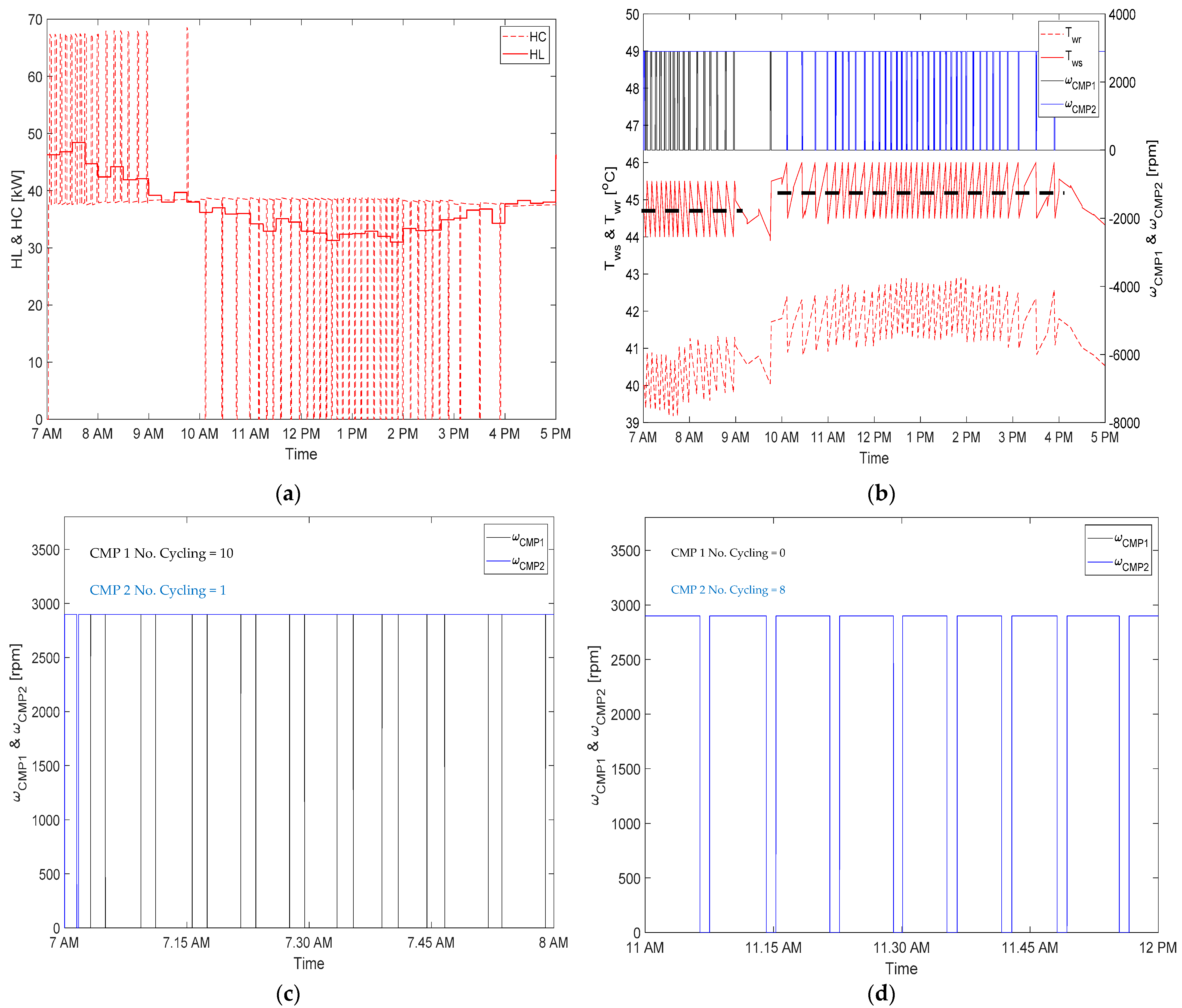
4.2. Results for the Constant-Speed Heat Pump with Sequential Control of Compressors

The results for the constant-speed HP in the high heating load day are shown in Figure 7a–d. In Figure 7a, the heating demand profile (red continuous line) is again presented together with the capacity delivered by the HP (dashed red line). The discontinuous pattern of the HC was due to the ON–OFF cycles of CMPs. In this respect, as shown in Figure 7b, it is worth noting that CMP1 (black line) operated only from 7 to 10 AM when the higher values of heating demand were observed. Then, after 10 am, CMP1 was always OFF, and CMP2 (blue line) was cycled to maintain the water supply temperature in the desired range. In addition, Figure 7b shows that the temperature of the water supplied to the building was oscillating around the value of 44.75 °C value (black dashed line), from 7 to 10 AM. After 10 AM, the temperature of the water supplied to the building was oscillating around the value of 45.25 °C values. This result was consequent to the band definitions for CMPs cycling shown in Table 5.

Figure 7c,d provides a focus on two hours in the high heating load day. More specifically, Figure 7c plots the CMPs’ operation from 7 to 8 AM, when the highest demand was observed. Conversely, Figure 7d focuses on CMPs’ operation from 1 PM to 2 PM when the lowest demand was observed. Looking at Figure 7c, CMP2 was ON for almost the whole hour; conversely, CMP1 cycled ON–OFF to meet the heating load. In addition, as indicated in Figure 7c, CMP1 cycled ON–OFF almost 10 times, which was less than the maximum threshold value equal to “12 cycles per hour” required for assuring a safe CMP operation. As shown in Figure 7d, from 1 PM to 2 PM, CMP1 was always OFF, and CMP2 was cycled to maintain the water supply temperature in the desired range. More specifically, CMP2 cycled ON–OFF almost eight times, which was less than the maximum threshold suggested by the manufacturer (i.e., 12). In Figure 7e, the mechanical power required by the CMPs is plotted. Figure 7f shows the average hourly COP values. The COP ranged between 4.42 and 4.75 during the operation due to the time-varying ODT values.

The simulation results for the constant-speed HP during the low heating load day are shown in Figure 8a–d. Like in Figure 7a, in Figure 8a, the heating demand profile (red continuous line) is again presented together with the capacity delivered by HP (dashed red line). It is worth noting that, differently from Figure 7a, the minimum value for HC was zero also during the first part of the day, and only one compressor (more specifically CMP2) was operating and cycling ON–OFF. As shown in Figure 8b, the temperature of the water supplied to the building was oscillating around the value of 45.25 °C value (black dashed line), following the range shown in Table 5. In Figure 8c,d, results for two hours on the assumed day are shown. More specifically, as shown in Figure 8c,d, during a high load hour (early morning from 7 to 8 AM), CMP1 operated for a few minutes between 7 and 7.15 AM. Then, CMP1 was always OFF, and CMP2 was cycled to maintain the water supply temperature in the desired range. As shown in Figure 8c,d, CMP2 was cycling ON-OFF almost 14 times in the early morning, and almost 15 times from 10 to 11 AM. In both hours, the number of CMP cycles was higher than the maximum threshold. In Figure 8e, the mechanical power required by the CMPs is plotted. As expected, it varied from 0 to 8.2 kW since only CMP was always ON. Figure 8f shows the average hourly COP values. The COP value ranged between 4.69 and 4.86 during the operation due to the different ODT values in the day.

The previous focus on CMPs’ operation highlighted the importance of including integrated modeling in studies that propose new design alternatives or control logic to increase energy savings or flexibility in buildings [41]. Indeed, in all these cases, any safety issues in HP operations can be easily predicted.

Effects of Hydraulic Inertia on the Operation of Constant-Speed HPs in Heating Mode

As explained in Section 2.1, the thermal inertia of the hydraulic loop was quantified by the C_s constant. As explained in Section 3.4, the C_s value was set to 1500 kJ/°C based on the HP’s nominal cooling capacity and the maximum cycles per hour in cooling mode. The previous analysis pointed out that, in the case of low heating demand, the number of CMP2 cycling was beyond the threshold value (see Figure 8b). It is, then, interesting to estimate the percentage variation in C_s when safety assessments were performed also including the heating mode. In this respect, the analysis considered a variation of C_s from the reference value (i.e., 1500 kJ/°C) to 2100 kJ/°C, with a step variation of +200 kJ/°C. As shown in Figure 9, the number of CMP2 cycling achieved the threshold values (i.e., 12 cycles per hour) when C_s increased from 1500 to 1900 kJ/°C (i.e., +26.67%). This result could be easily explained by considering the criterion followed to size the HP. Indeed, since the HP was sized based on cooling demand, during the winter, the heating capacity delivered by the HP was likely to be higher than the heating demand (which for the considered locality was very close to the cooling one). Then, due to the HP oversizing, several cycles were needed in hours characterized by a low heating load.

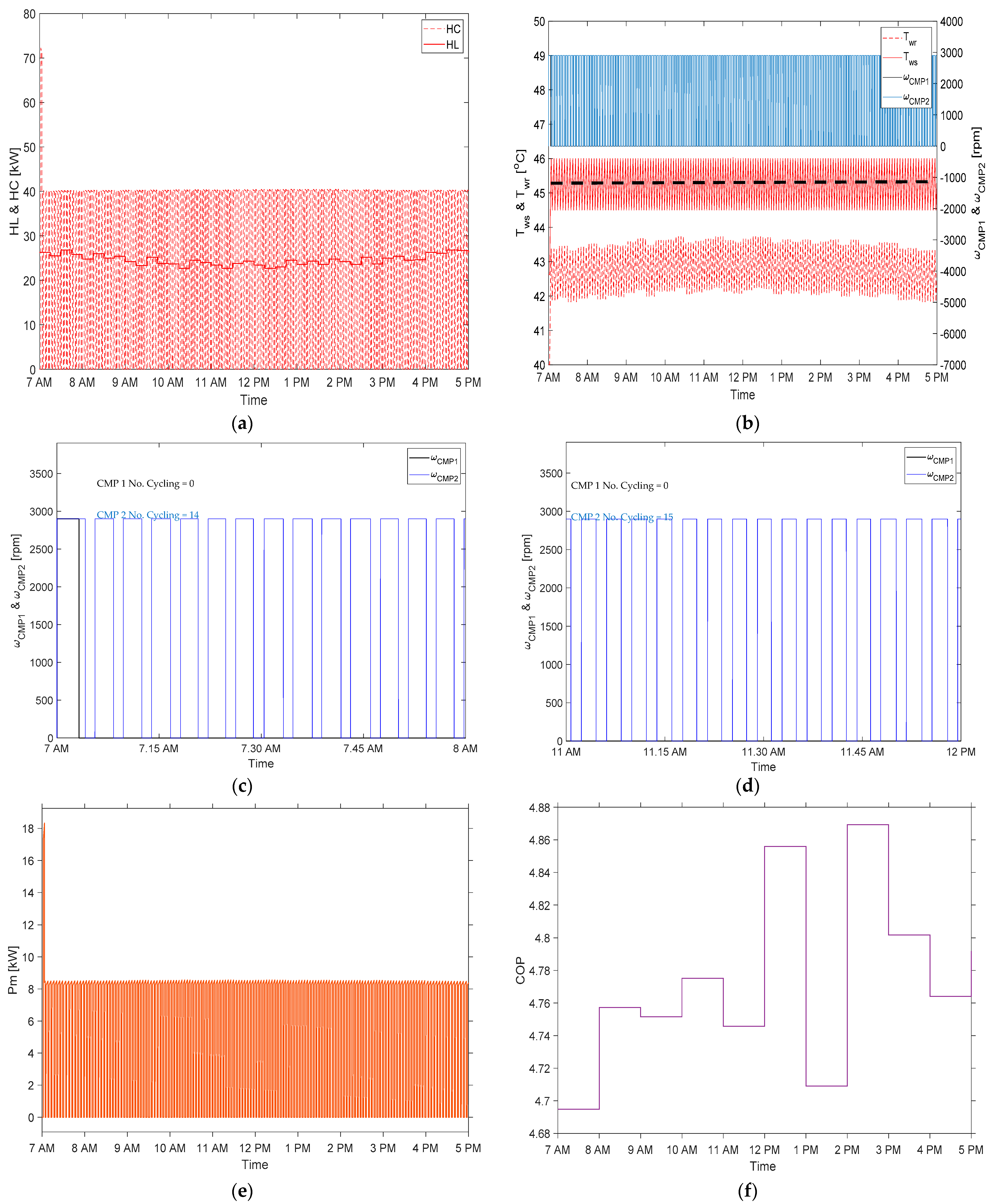
4.3. Analysis of the HP Operation Based on “Heating Curve”

As explained in Section 3.3, the HP was operated by setting a variable setpoint for the temperature of the water supplied to the building, according to the heating curve shown in Figure 5b. Results for the high heating load day are shown in Figure 10a,b. Each figure compares the results obtained in the case of a “constant” set point for T_ws with the case of a “variable” setpoint. As shown in Figure 10a, due to the new control strategy, the controller did not maintain the T_ws at 45 °C, as shown in Figure 6b. More specifically, the values of T_ws varied from about 40 °C in the early morning to around 41.5 °C at 4 PM. As shown in Figure 10b, an increase in the average value of COP was achieved by this new strategy (orange line) compared to the strategy with a constant T_ws,ref (purple line).

Results for the low-heating load day are shown in Figure 10c,d. In this case, since ODT was always higher than 15 °C (as shown in Figure 10a), the water was supplied to a T_ws value lower than 40 °C, with a substantial increase in the average COP value throughout the day (Figure 10d).

Before concluding, it is worth noting that this analysis focused more on the effect of this strategy on HP operation and energy performance, without considering two possible side effects. First, changes in occupants’ comfort conditions were not considered, as evidenced by the absence of typical metrics proposed by International Standards [64]. Second, the effects of such a strategy on the controller action of each heating device (installed within the building) were not considered. Indeed, local thermostats could force fan coil fans to run for an extended time to meet the same heating load, thus reducing the benefits gained from a higher-performing HP. Only a comprehensive analysis, in which the modeling proposed here was solved together with (i) building and heating system modeling and (ii) metrics for assessing occupant comfort, could provide a complete answer to the feasibility of any new management strategy.

4.4. Analysis of the Response of HPs in the Case of Low-Temperature Heating Devices

In this subsection, results of the analysis of the dynamic response of both variable-speed and constant-speed HPs when supplying low-temperature heating devices such as heating floors are shown.

Figure 11a,b shows results for the variable-speed HP on the high heating load day. As shown in Figure 11a, T_ws was maintained at 35 °C (i.e., the assumed HP setpoint when supplying the heating floor) by the action of the controller. Moreover, the rotating speed of the CMPs varied from about 1000 rpm to 1400 rpm during the day, due to changes in the heating demand. However, note that CMPs speed was lower than the one observed for the variable-speed HP when supplying fan coils (see Figure 6b) with a reference set-point of 45 °C (i.e., from 2000 rpm to 4000 rpm). The lower CMP speeds led, in turn, to higher COP values (almost +50%). Indeed, as shown in Figure 11b, the COP ranged between 8.5 and 9.6. The COP values in the case of the HPs serving fan coils ranged between 4.23 and 5.05 (see Figure 6d).

Results for the constant-speed HP operation in the low-load heating day are shown in Figure 12a–d. As shown in Figure 12a, T_ws varied around 35 °C due to the cycling of CMPs. Moreover, CMP1 was always OFF, while CMP2 was the one responsible to meet the user’s demand. As shown in Figure 12b, the COP ranged between 6.25 and 6.5. These COP values were higher than the ones found in the case of the HPs serving fan coils, which ranged between 4.69 and 4.86 (see Figure 8f). Before ending, it is useful to provide insights into the number of CMP2 cycling in two typical hours of the day. In this respect, Figure 12c provides a zoom on CMP operation from 7 AM to 8 AM. In this hour, CMP2 cycled almost 11 times. The number of cycling became even higher (and beyond the threshold value) from 10 AM to 11 AM, as shown in Figure 12d. It is worth mentioning again that these results were found assuming a Cs value of 1900 kJ/°C. Then, when the operating temperature of the supplied heating devices was reduced, the effect of HP “oversizing” heavily affected CMPs’ operation. To reduce the number of CMP2 cycling, an even higher C_s value was then required.

5. Conclusions

This work proposed an integrated thermodynamic and control modeling of an air-to-water HP to assess the energy saving achieved by new control strategies or innovative applications of HPs in buildings. Meantime, the dynamic response of the HP and the steady-state operation was fully monitored. To show these capabilities, a reversible air-to-water HP serving an office in the Mediterranean area was investigated. The results show that, in the case of a variable-speed operation, the model allowed for monitoring the controller action on the HP, such as the instantaneous CMP speed, the meeting of the required setpoint, the time needed to reach a steady state operation after heating demand variation, and water supply overshoot. In the case of a constant-speed HP, the number of CMP cycling was monitored. More specifically, on low heating load day, the model predicted that the number of CMP cycling was well beyond the permitted threshold. Then, the possibility to perform safety analysis on CMP operations was enabled. More specifically, the great sensitivity of HP response to the different amounts of water in the hydronic loop was quantified. In this respect, a different amount of water in the hydronic loop was required to maintain the compressor cycling below the threshold value in cooling and heating mode (+26.67%). Thanks to the proposed model, the effect of alternative operating strategies on dynamic response and steady-state operation could be simulated. In this respect, the one based on heating curves was considered only for the case of the variable-speed HP. In this respect, it was found that an increase of about 50 % in the COP value was achieved on moderately cold days. Finally, the analysis of the effects of the low-temperature heating device revealed an increase in the energy performance of the HP, but some issues for CMP2 were raised due to the increased number of ON–OFF cycling. All the insights gained by the adoption of an integrated model will provide precious support in the studies where the description of the dynamic response is necessary (e.g., use of HPs for ancillary services provision). Moreover, thanks to the possibility to monitor HP operations, the feasibility of new control logic aimed at increasing energy savings or flexibility could be verified. Future works will apply the proposed model to the case of energy-saving assessment achievable by DR programs using reversible air-to-water HPs.

References

1. International Energy Agency (IEA). Heating; IEA: Paris, France, 2022. [Google Scholar]
2. Ehsan, A.; Preece, R. Quantifying the Impacts of Heat Decarbonisation Pathways on the Future Electricity and Gas Demand. Energy 2022, 254, 124229. [Google Scholar] [CrossRef]
3. Nowak, T. European Heat Pump Market. 2021. Available online: https://www.ehpa.org/ (accessed on 21 January 2023).
4. European Union. Commission Communication from the Commission to the European Parliament, The European Council, The Council, The European Economic and Social Committee and the Committee of the Regions 2022. Available online: https://www.eea.europa.eu/policy-documents/communication-from-the-commission-to-1 (accessed on 22 January 2023).
5. Østergaard, P.A.; Lund, H.; Thellufsen, J.Z.; Sorknæs, P.; Mathiesen, B. V Review and Validation of EnergyPLAN. Renew. Sustain. Energy Rev. 2022, 168, 112724. [Google Scholar] [CrossRef]
6. Mathiesen, B.V.; Lund, H.; Connolly, D.; Wenzel, H.; Østergaard, P.A.; Möller, B.; Nielsen, S.; Ridjan, I.; Karnøe, P.; Sperling, K.; et al. Smart Energy Systems for Coherent 100% Renewable Energy and Transport Solutions. Appl. Energy 2015, 145, 139–154. [Google Scholar] [CrossRef]
7. Bashir, A.A.; Lund, A.; Pourakbari-Kasmaei, M.; Lehtonen, M. Optimizing Power and Heat Sector Coupling for the Implementation of Carbon-Free Communities. Energies 2021, 14, 1911. [Google Scholar] [CrossRef]
8. Fischer, D.; Madani, H. On Heat Pumps in Smart Grids: A Review. Renew. Sustain. Energy Rev. 2017, 70, 342–357. [Google Scholar] [CrossRef]
9. Posma, J.; Lampropoulos, I.; Schram, W.; van Sark, W. Provision of Ancillary Services from an Aggregated Portfolio of Residential Heat Pumps on the Dutch Frequency Containment Reserve Market. Appl. Sci. 2019, 9, 590. [Google Scholar] [CrossRef]
10. Gjorgievski, V.Z.; Markovska, N.; Abazi, A.; Duić, N. The Potential of Power-to-Heat Demand Response to Improve the Flexibility of the Energy System: An Empirical Review. Renew. Sustain. Energy Rev. 2021, 138, 110489. [Google Scholar] [CrossRef]
11. Guelpa, E.; Verda, V. Demand Response and Other Demand Side Management Techniques for District Heating: A Review. Energy 2021, 219, 119440. [Google Scholar] [CrossRef]
12. Salpakari, J.; Mikkola, J.; Lund, P.D. Improved Flexibility with Large-Scale Variable Renewable Power in Cities through Optimal Demand Side Management and Power-to-Heat Conversion. Energy Convers. Manag. 2016, 126, 649–661. [Google Scholar] [CrossRef]
13. Lund, H.; Østergaard, P.A.; Nielsen, T.B.; Werner, S.; Thorsen, J.E.; Gudmundsson, O.; Arabkoohsar, A.; Mathiesen, B.V. Perspectives on Fourth and Fifth Generation District Heating. Energy 2021, 227, 120520. [Google Scholar] [CrossRef]
14. D’Ettorre, F.; De Rosa, M.; Conti, P.; Testi, D.; Finn, D. Mapping the Energy Flexibility Potential of Single Buildings Equipped with Optimally-Controlled Heat Pump, Gas Boilers and Thermal Storage. Sustain. Cities Soc. 2019, 50, 101689. [Google Scholar] [CrossRef]
15. Péan, T. Heat Pump Controls to Exploit the Energy Flexibility of Building Thermal Loads; Springer: Berlin/Heidelberg, Germany, 2020. [Google Scholar]
16. Sperber, E.; Frey, U.; Bertsch, V. Reduced-Order Models for Assessing Demand Response with Heat Pumps—Insights from the German Energy System. Energy Build. 2020, 223, 110144. [Google Scholar] [CrossRef]
17. Zhang, L.; Good, N.; Mancarella, P. Building-to-Grid Flexibility: Modelling and Assessment Metrics for Residential Demand Response from Heat Pump Aggregations. Appl. Energy 2019, 233–234, 709–723. [Google Scholar] [CrossRef]
18. Zanetti, E.; Azzolin, M.; Bortolin, S.; Busato, G.; Del Col, D. Experimental Data and Modelling of a Dual Source Reversible Heat Pump Equipped with a Minichannels Evaporator. Therm. Sci. Eng. Prog. 2022, 35, 101471. [Google Scholar] [CrossRef]
19. Puttige, A.R.; Andersson, S.; Östin, R.; Olofsson, T. Application of Regression and ANN Models for Heat Pumps with Field Measurements. Energies 2021, 14, 1750. [Google Scholar] [CrossRef]
20. Puttige, A.R.; Andersson, S.; Östin, R.; Olofsson, T. Modeling and Optimization of Hybrid Ground Source Heat Pump with District Heating and Cooling. Energy Build. 2022, 264, 112065. [Google Scholar] [CrossRef]
21. Maier, L.; Schönegge, M.; Henn, S.; Hering, D.; Müller, D. Assessing Mixed-Integer-Based Heat Pump Modeling Approaches for Model Predictive Control Applications in Buildings. Appl. Energy 2022, 326, 119894. [Google Scholar] [CrossRef]
22. Liu, H.; Cai, J. A Robust Gray-Box Modeling Methodology for Variable-Speed Direct-Expansion Systems with Limited Training Data. Int. J. Refrig. 2021, 129, 128–138. [Google Scholar] [CrossRef]
23. Artuso, P.; Tosato, G.; Rossetti, A.; Marinetti, S.; Hafner, A.; Banasiak, K.; Minetto, S. Dynamic Modelling and Validation of an Air-to-Water Reversible R744 Heat Pump for High Energy Demand Buildings. Energies 2021, 14, 8238. [Google Scholar] [CrossRef]
24. Xu, Z.; Sun, X.; Li, X.; Wang, Z.; Xu, W.; Shao, S.; Xu, C.; Yang, Q.; Li, H.; Zhao, W. On-off Cycling Model Featured with Pattern Recognition of Air-to-Water Heat Pumps. Appl. Therm. Eng. 2021, 196, 117317. [Google Scholar] [CrossRef]
25. Kim, Y.-J.; Norford, L.K.; Kirtley, J.L. Modeling and Analysis of a Variable Speed Heat Pump for Frequency Regulation through Direct Load Control. IEEE Trans. Power Syst. 2015, 30, 397–408. [Google Scholar] [CrossRef]
26. Abid, M.; Hewitt, N.; Huang, M.-J.; Wilson, C.; Cotter, D. Domestic Retrofit Assessment of the Heat Pump System Considering the Impact of Heat Supply Temperature and Operating Mode of Control—A Case Study. Sustainability 2021, 13, 10857. [Google Scholar] [CrossRef]
27. Zakula, T.; Gayeski, N.T.; Armstrong, P.R.; Norford, L.K. Variable-Speed Heat Pump Model for a Wide Range of Cooling Conditions and Loads. Hvacr Res. 2011, 17, 670–691. [Google Scholar] [CrossRef]
28. Ma, J.; Kim, D.; Braun, J.E.; Horton, W.T. Development and Validation of a Dynamic Modeling Framework for Air-Source Heat Pumps under Cycling of Frosting and Reverse-Cycle Defrosting. Energy 2023, 272, 127030. [Google Scholar] [CrossRef]
29. Roccatello, E.; Prada, A.; Baggio, P.; Baratieri, M. Impact of Startup and Defrosting on the Modeling of Hybrid Systems in Building Energy Simulations. J. Build. Eng. 2023, 65, 105767. [Google Scholar] [CrossRef]
30. Rossi di Schio, E.; Ballerini, V.; Dongellini, M.; Valdiserri, P. Defrosting of Air-Source Heat Pumps: Effect of Real Temperature Data on Seasonal Energy Performance for Different Locations in Italy. Appl. Sci. 2021, 11, 8003. [Google Scholar] [CrossRef]
31. Sezen, K.; Gungor, A. Performance Analysis of Air Source Heat Pump According to Outside Temperature and Relative Humidity with Mathematical Modeling. Energy Convers. Manag. 2022, 263, 115702. [Google Scholar] [CrossRef]
32. Popovac, M.; Emhofer, J.; Reichl, C. Frosting in a Heat Pump Evaporator Part B: Numerical Analysis. Appl. Therm. Eng. 2021, 199, 117488. [Google Scholar] [CrossRef]
33. Bagarella, G.; Lazzarin, R.; Noro, M. Sizing Strategy of on–off and Modulating Heat Pump Systems Based on Annual Energy Analysis. Int. J. Refrig. 2016, 65, 183–193. [Google Scholar] [CrossRef]
34. Liu, S.; Bai, X.; Deng, S.; Zhang, L.; Wei, M. A Modeling Study on Developing the Condensing-Frosting Performance Maps for a Variable Speed Air Source Heat Pump. J. Build. Eng. 2022, 58, 104990. [Google Scholar] [CrossRef]
35. Harild Rasmussen, T.B.; Wu, Q.; Zhang, M. Primary Frequency Support from Local Control of Large-Scale Heat Pumps. Int. J. Electr. Power Energy Syst. 2021, 133, 107270. [Google Scholar] [CrossRef]
36. Bechtel, S.; Rafii-Tabrizi, S.; Scholzen, F.; Hadji-Minaglou, J.-R.; Maas, S. Influence of Thermal Energy Storage and Heat Pump Parametrization for Demand-Side-Management in a Nearly-Zero-Energy-Building Using Model Predictive Control. Energy Build. 2020, 226, 110364. [Google Scholar] [CrossRef]
37. Ding, Y.; Bai, Y.; Tian, Z.; Wang, Q.; Su, H. Coordinated Optimization of Robustness and Flexibility of Building Heating Systems for Demand Response Control Considering Prediction Uncertainty. Appl. Therm. Eng. 2023, 223, 120024. [Google Scholar] [CrossRef]
38. Abokersh, M.H.; Saikia, K.; Cabeza, L.F.; Boer, D.; Vallès, M. Flexible Heat Pump Integration to Improve Sustainable Transition toward 4th Generation District Heating. Energy Convers. Manag. 2020, 225, 113379. [Google Scholar] [CrossRef]
39. Montrose, R.S.; Gardner, J.F.; Satici, A.C. Centralized and Decentralized Optimal Control of Variable Speed Heat Pumps. Energies 2021, 14, 4012. [Google Scholar] [CrossRef]
40. Lee, Z.; Gupta, K.; Kircher, K.J.; Zhang, K.M. Mixed-Integer Model Predictive Control of Variable-Speed Heat Pumps. Energy Build. 2019, 198, 75–83. [Google Scholar] [CrossRef]
41. Dengiz, T.; Jochem, P.; Fichtner, W. Demand Response with Heuristic Control Strategies for Modulating Heat Pumps. Appl. Energy 2019, 238, 1346–1360. [Google Scholar] [CrossRef]
42. Baeten, B.; Rogiers, F.; Helsen, L. Reduction of Heat Pump Induced Peak Electricity Use and Required Generation Capacity through Thermal Energy Storage and Demand Response. Appl. Energy 2017, 195, 184–195. [Google Scholar] [CrossRef]
43. Efkarpidis, N.A.; Vomva, S.A.; Christoforidis, G.C.; Papagiannis, G.K. Optimal Day-to-Day Scheduling of Multiple Energy Assets in Residential Buildings Equipped with Variable-Speed Heat Pumps. Appl. Energy 2022, 312, 118702. [Google Scholar] [CrossRef]
44. Arteconi, A.; Polonara, F. Assessing the Demand Side Management Potential and the Energy Flexibility of Heat Pumps in Buildings. Energies 2018, 11, 1846. [Google Scholar] [CrossRef]
45. Schibuola, L.; Scarpa, M.; Tambani, C. Demand Response Management by Means of Heat Pumps Controlled via Real Time Pricing. Energy Build. 2015, 90, 15–28. [Google Scholar] [CrossRef]
46. Meesenburg, W.; Markussen, W.B.; Ommen, T.; Elmegaard, B. Optimizing Control of Two-Stage Ammonia Heat Pump for Fast Regulation of Power Uptake. Appl. Energy 2020, 271, 115126. [Google Scholar] [CrossRef]
47. Manner, P.; Alapera, I.; Honkapuro, S. Domestic Heat Pumps as a Source of Primary Frequency Control Reserve. In Proceedings of the 2020 17th International Conference on the European Energy Market (EEM), Stockholm, Sweden, 16–18 September 2020. [Google Scholar] [CrossRef]
48. Romero Rodríguez, L.; Brennenstuhl, M.; Yadack, M.; Boch, P.; Eicker, U. Heuristic Optimization of Clusters of Heat Pumps: A Simulation and Case Study of Residential Frequency Reserve. Appl. Energy 2019, 233–234, 943–958. [Google Scholar] [CrossRef]
49. Bartolucci, L.; Cordiner, S.; Mulone, V.; Santarelli, M. Ancillary Services Provided by Hybrid Residential Renewable Energy Systems through Thermal and Electrochemical Storage Systems. Energies 2019, 12, 2429. [Google Scholar] [CrossRef]
50. Szreder, M.; Miara, M. Effect of Heat Capacity Modulation of Heat Pump to Meet Variable Hot Water Demand. Appl. Therm. Eng. 2020, 165, 114591. [Google Scholar] [CrossRef]
51. Liu, H.; Cai, J. Improved Superheat Control of Variable-Speed Vapor Compression Systems in Provision of Fast Load Balancing Services. Int. J. Refrig. 2021, 132, 187–196. [Google Scholar] [CrossRef]
52. Clauß, J.; Georges, L. Model Complexity of Heat Pump Systems to Investigate the Building Energy Flexibility and Guidelines for Model Implementation. Appl. Energy 2019, 255, 113847. [Google Scholar] [CrossRef]
53. Bagarella, G.; Lazzarin, R.M.; Lamanna, B. Cycling Losses in Refrigeration Equipment: An Experimental Evaluation. Int. J. Refrig. 2013, 36, 2111–2118. [Google Scholar] [CrossRef]
54. Michele, V.; Diego, D. Le Centrali Frigorifere; Editoriale Delfino: Milano, Italy, 2015. [Google Scholar]
55. Cirrincione, M.; Pucci, M.; Vitale, G. Power Converters and AC Electrical Drives with Linear Neural Networks; CRC Press: Boca Raton, FL, USA, 2016. [Google Scholar]
56. Piacentino, A.; Barbaro, C. A Comprehensive Tool for Efficient Design and Operation of Polygeneration-Based Energy Μgrids Serving a Cluster of Buildings. Part II: Analysis of the Applicative Potential. Appl. Energy 2013, 111, 1222–1238. [Google Scholar] [CrossRef]
57. Meteonorm: Meteonorm, Global Meteorological Database; Version 7.1.7.201517; Handbook Part II: Theory; PVsyst: Satigny, Switzerland, 2015.
58. IMST-Art; v.4.0; IMST-Group Instituto de Ingeniería Energética Universidad Politécnica de Valencia: Valencia, Spain, 2021.
59. Blanco Castro, J.; Urchueguía, J.F.; Corberán, J.M.; Gonzálvez, J. Optimized Design of a Heat Exchanger for an Air-to-Water Reversible Heat Pump Working with Propane (R290) as Refrigerant: Modelling Analysis and Experimental Observations. Appl. Therm. Eng 2005, 25, 2450–2462. [Google Scholar] [CrossRef]
60. Braun, J.E.; Klein, S.A.; Mitchell, J.W. Effictiveness Models for Cooling Towers and Cooling Coils; ASHRAE Transactions: Peachtree Corners, GA, USA, 1989; Volume 95, Part 2. [Google Scholar]
61. Sabiana, “Carisma” Fan Coils. Available online: https://www.sabiana.it/it/products/carisma-crc (accessed on 12 December 2022).
62. MathWorks MATLAB; v.R2022b; MathWorks: Natick, MA, USA, 2022.
63. Kumar, M.D.; Catrini, P.; Piacentino, A.; Cirrincione, M. Advanced Modeling and Energy-Saving-Oriented Assessment of Control Strategies for Air-Cooled Chillers in Space Cooling Applications. Energy Convers. Manag. 2023. under review. [Google Scholar]
64. Olesen, B.W.; Parsons, K.C. Introduction to thermal comfort standards and to the proposed new version of EN ISO 7730. Energy Build. 2002, 34, 537–549. [Google Scholar] [CrossRef]
Figure 1. Simplified scheme of a reversible air-to-water HP.
Sustainability 15 08664 g001
Figure 2. Schematic of the control for a variable speed air-to-water HP.
Sustainability 15 08664 g002
Figure 3. (a) Schematic of the control for a variable-speed air-to-water HP; (b) activation control for an HP equipped with two constant-speed CMPs.
Sustainability 15 08664 g003aSustainability 15 08664 g003b
Figure 4. Profiles of typical low- and high-heating load days: (a) ODT values, (b) heating demand.
Sustainability 15 08664 g004
Figure 5. (a) Sensitivity of fan coil’s heating capacity to the supplied water temperature and (b) supply hot water temperature set point vs. ODT.
Sustainability 15 08664 g005
Figure 6. Results for the variable-speed HP in the high heating load day: (a) Heating load and heating capacity, (b) water supply temperature, water return temperature, and compressor speed, (c) mechanical power, (d) COP.
Sustainability 15 08664 g006
Figure 7. SC results for the high-heating load day: (a) Heating Load and Heating Capacity (b) Water supply, Water return temperature, and CMPs cycles, (c) CMPs’ operation from 7–8 am, (d) CMPs’ operation from 1–2 PM, (e) Mechanical Power, and (f) COP.
Sustainability 15 08664 g007aSustainability 15 08664 g007b
Figure 8. Results for the low-heating load day: (a) Heating Load and Heating Capacity (b) Water supply, Water return temperature, and CMPs cycles, (c) CMPs’ operation from 7 to 8 am, (d) CMPs’ operation from 10 to 11 am, (e) Mechanical Power, and (f) COP.
Sustainability 15 08664 g008
Figure 9. Variation of hydraulic loop inertia for a safe CMP operation in heating mode.
Sustainability 15 08664 g009
Figure 10. Results of HP operation when operated following the developed “heating curve”: (a) Water supply, Water return temperature, and compressor speed in the high heating load day; (b) COP values in the high heating load day; (c) Water supply, Water return temperature, and Compressor speed in the low heating load day; (d) COP values in the low heating load day.
Sustainability 15 08664 g010
Figure 11. Analysis of the dynamic response of variable speed HP with the low-temperature heating device in the high heating load day: (a) Water supply, Water return temperature, and Compressor speed; (b) COP values.
Sustainability 15 08664 g011
Figure 12. Analysis of the dynamic response of constant-speed HP in the case of low-temperature heating devices during the low heating load day: (a) Water supply, Water return temperature, and Compressor speed; (b) COP values; (c) CMPs’ operation from 7 to 8 am, (d) CMPs’ operation from 10 to 11 am.
Sustainability 15 08664 g012