Article

Analysis of Traffic Characteristics and Distance Optimization Design between Entrances and Exits of Urban Construction Projects and Adjacent Planar Intersections

School of Civil Engineering and Architecture, Wuhan Institute of Technology, Wuhan 430074, China
*
Author to whom correspondence should be addressed.
Sustainability 2023, 15(11), 8656; https://doi.org/10.3390/su15118656
Submission received: 20 March 2023 / Revised: 18 May 2023 / Accepted: 23 May 2023 / Published: 26 May 2023
(This article belongs to the Section Sustainable Transportation)

Abstract

:
Motor vehicle entrances/exits ensure the accessibility of traffic within urban construction projects, but the improper distance between adjacent sections can lead to vehicle queues at upstream or downstream intersections, causing congestion within the influence of the entrances and exits. It is necessary to improve the operational efficiency of entrances/exits and intersections of urban construction projects. The calculation models of the vehicle convergence section, intertwined section and queuing section are established based on the data fitting relationship curve, function relationship fitting and maximum likelihood estimation method. These are combined with the traffic characteristics of vehicles and a statistical analysis of traffic flow survey data, and the models are developed according to the equal speed offset cosine curve function, queuing theory and traffic flow fluctuation theory. Based on the analysis of the traffic flow characteristics, the minimum distance value is calculated, and the recommended value is obtained. The VISSIM simulation parameters are calibrated according to the survey data, and then the simulation is carried out and the results are output. The results show that the output values of each index are improved under the calculated distance, indicating that the study has certain significance for improving the traffic conditions and operational efficiency at entrances/exists and intersections, which verifies the applicability and effectiveness of the theoretical model proposed in this paper.

1. Introduction

In recent years, with the accelerating urbanization process, more high-intensity and high-density land development has emerged, and the development scale of construction projects has gradually expanded [1,2]. Due to the large scale of construction of some projects, traffic volume and traffic attraction increase rapidly, and due to the irregular setting of entrances and exits, it is easy for traffic to become congested at entrances and exits, causing the traffic efficiency of adjacent sections and the regional road network to decrease significantly [3,4]. The connection between the entrances and exits of urban construction projects and intersections is an important part of the operational efficiency of the regional road network system. The reasonable setting of entrances and exits for urban construction projects can effectively improve traffic congestion, reduce traffic conflict points and improve and ensure the efficiency and safety of urban road traffic operation [5,6].
In terms of traffic data acquisition, short-term traffic volumes are better suited for prediction with models based on Bayesian Combined Neural Networks (BCNN) or Discrete Wavelet Transform (DWT) [7,8]. The XGBoost, LSTM and GRU models developed by Mahmoud [9] measured values closer to real values in the field. Traffic light intersection data detection schemes using edge computing, or load redistribution strategies using rational allocation of congestion load, are more suitable for complex and variable intersections [10,11]. The queue length was analyzed to determine the optimal value of green time [12]. To address the issue of queue length at intersections, both single and multiple, an improved version of the sparrow algorithm was developed. The algorithm is designed to reduce queue length, while ensuring both accuracy and safety [13]. Considering mixed traffic with different vehicle types and traffic directions, the use of microsimulation models [14], or short-term queue length prediction models, can optimally adjust the signal phase and timing of traffic movements to reduce stopping delays due to long intersection cycles [15,16]. When predicting queue length, the concept of equivalent queue length optimizes calculation errors [17]. Due to the stationary and dynamic movement of vehicles, more accurate vehicle delay data can be obtained if the vehicle arrival time is divided into different periods [18]. Palumbo [19] created a framework for accurate traffic analysis to estimate the observed vehicle queue lengths on the roadway, and to adjust the timing of each phase of the intersection signal to improve vehicle delays. Considering that unsignalized intersections are still the majority, AnyLogic software is more suitable for their capacity calculation than the traditional HCM and Harders/Seigloch formulas [20]. Zeng [21] approached the queuing problem from the perspective of intelligent driving. They believed that increasing the proportion of intelligent connected vehicles and queue size can increase the maximum traffic volume, and an appropriate queue size can reduce average energy consumption. In addition to queuing sections, for intertwined sections with significant vehicle conflicts, the length, lane continuity and the number of lanes can also have a significant impact on the level of service, safety performance and distance between entrances and intersections [22,23]. In intertwined sections, vehicles on major roads were also more likely to change lanes earlier than vehicles on minor roads [24]. Li [25] established a merging probability model and a driving distance distribution probability model for ramp vehicles using probability analysis and microscopic simulation, and the models were verified by empirical testing. If the weaving area was a U-shaped lane, sufficient weaving length is required to improve the performance of the weaving section and to ensure the safety of road users [26]. The analytical calculation of queueing section length and weaving section length is crucial for building the distance analysis model.
The establishment of a suitable theoretical model to analyze the influence brought by different traffic elements is essential for the optimal design of distances. Huang [27] used an ant colony algorithm and swarm decision theory to control the two factors affecting adjacent intersection distance and road segment traffic flow saturation. They searched for and optimized the shortest path, and thus established a model of an urban road network. The speed–distance and time–distance relationship models established can provide a reference for the minimum spacing criteria [28]. For different lane spacing, the impact of the minimum spacing of access sections on traffic safety varies [29,30]. For Automated Truck Lanes (ATL), the recommended values for the location and length of the entrances and exits should also be provided [31]. A new type of intersection that combines the advantages of left-turn control and tandem control can be used as an alternative to conventional intersections, where minimum spacing is insufficient or lanes are limited [32]. The impact of different urban construction projects on traffic varies, with the number of bus stops and distance to the nearest school negatively correlated to road speeds [33], while arterial road sections adjacent to commercial land used tend to have higher crash rates [34]. For the entrances themselves, Williams [35] believed that entrance management is a systematic and coordinated control of site development and road planning and design, which involves all stages of planning, design and operation. A series of management measures were proposed to improve and ensure road safety and traffic flow.
In the literature, the entrance/exit distances were mostly based on theoretical derivation, lacking systematic practical data support and unified technical standards. When selecting the relevant parameters, most study authors are limited to theoretical experience, without taking values and calculating results according to the actual traffic operation, and the research into the entrance/exit settings of urban construction projects needs to be more comprehensive and in-depth. Based on actual traffic operation, this paper analyzed the behavior of traffic flow characteristics, headway time distance and vehicle lane change based on actual survey data. The results from this analysis are applied to the calculation of the model and the recommended values are given. The motor vehicle entrances and exits of selected construction projects were taken as the object of study, defined as T-shaped intersections formed by intersections with urban roads for motor vehicle access. For the problem of insufficient distance between the entrances/exits and the adjacent level intersection, through field investigation of the current traffic, the selection of theoretical research methods and the comparison of theoretical and actual traffic simulation were combined. We analyzed the factors that influence the distance between entrances and intersections, established a calculation model for this distance, and then used survey data and the results of traffic flow characteristic analysis to calculate the recommended values. The VISSIM software was used to simulate and evaluate the effect of the theoretical model by comparing the output value of the index under the condition of the current length and the condition of the calculated length. This work was carried out to verify the validity of the theoretical model calculation values, and to provide guidance for improving the overall operation of urban traffic.
Despite the extensive research on vehicle entrances and intersections, there remains a lack of systematic practical data support or unified technical standards for determining the appropriate distances between them. The innovation of this study is that it provides a new method for determining the appropriate distances between entrances/exits and intersections, based on actual survey data and analysis of traffic flow characteristics and behaviors. It contributes to the overall operation of urban traffic.
This study encompasses several aspects. Firstly, urban road intersections and entrances/exits are categorized according to traffic characteristics and factors influencing the distances between them are analyzed, including vehicle speed, traffic composition, lane number and intersection signal timing. Secondly, a distance model between construction project entrances/exits and different intersections is established. Finally, the validity of the model is verified by VISSIM simulation.

2. Data Acquisition and Analysis

2.1. Traffic Survey

This survey used the AxleLight roadside laser surveyor to record and collect data on vehicle travel speed, traffic flow and vehicle type. Combined with the current situation of traffic congestion at the entrances/exits of urban construction projects and adjacent planes in Wuhan, the intersection of Youyi Avenue and Wuhan Avenue in Wuhan City was selected, and the entrances/exits of Junlin International and The Shopping Mall were selected as the main investigation sites. The traffic volume survey adopted the traditional video survey method, and the data acquisition instruments include: a roadside laser survey instrument, multi-function traffic data counter, push ruler, camera, etc.
The map of the selected survey site is shown in Figure 1. The arrow points to the location of the entrances/exits. There are two entrances/exits of The Shopping Mall, and they are referred to as A and B to distinguish them. The basic information of the survey area is as follows: Wuhan Avenue has six lanes in both directions and Youyi Avenue has eight lanes in both directions. The vehicle types of the intersection are mainly composed of cars, buses and pickup trucks. The distance between the entrance and exit of Junlin International and the intersection is 95 m. The distance between the entrance/exit A of The Shopping Mall and intersection is 135 m, and the distance between the entrance/exit A and B is 65 m. The traffic survey was conducted on Tuesday, 15 November 2022. According to the characteristics of urban traffic time, the traffic flow in the evening rush hour is large and the contradiction is more prominent. Therefore, 17:00–19:00 of the evening rush hour was selected for observation.

2.2. Analysis of Traffic Characteristics of Project Entrances/Exits and Intersections

2.2.1. Traffic Characteristics Analysis

  • Traffic volume characteristics
Through the analysis of the traffic volume characteristics of the planar intersection, it can be concluded that there is a high demand for vehicles going straight and turning left. The road section is eight lanes in both directions, and the vehicles going straight occupy two lanes, leading to a long line of vehicles going straight in the space. When the queue length is too long, queue-jumping vehicles will affect other lanes, resulting in slow passage in other directions. The traffic volume of each lane was larger during peak hours compared to other hours, and the service level of each lane tends to be saturated, which will generate congestion queues. Therefore, the calculation model of the queue length of the intersection needs to be established. The investigation results are shown in Table 1.
By analyzing of the traffic volume characteristics of the entrances and exits, it can be seen that the entrances and exits of The Shopping Mall were saturated with incoming and outgoing vehicles, resulting in a queue of vehicles on Wuhan Avenue and a large number of vehicles leading to the intersection, affecting the normal flow of mainline traffic. The vehicle queue length at the north entrance stop line of the Wuhan Avenue Youyi Avenue intersection exceeded that of the entrance and exit of the Junlin International, resulting in the blockage of the entrances/exits and affecting normal vehicle access. Therefore, the smooth operation of the main road is highly dependent on the normal access of traffic through the entrances and exits. Due to the large volume of peak traffic, the vehicle queue length at the intersection often exceeds the capacity of the entrance and exit, which in turn impedes vehicle access. To address this issue, we conducted an analysis of the queue characteristics of the entrance and exit and established a model to calculate the queue length of the entrance and exit. The results of the survey are shown in Figure 2.
b.
Vehicle speed characteristics
Speed is the ratio of the distance traveled by the vehicle on the road to the time, and is also a traffic parameter that visually reflects the operational efficiency of the road, the degree of road congestion and traffic delays, etc., [36,37]. According to the speed distribution of different cross-sections obtained from the statistics, the conclusion is as follows: speed is reduced with the intersection stop line distance, due to the queue of vehicles or the presence of a red-light passage, and a vehicle will gradually slow down until its speed is reduced to zero. During this period, the distance between the vehicles was small, making them prone to collision accidents. To ensure that the vehicle can safely and smoothly drive in or out at the entrance or exit, the vehicle tends to slow down accordingly, so when the vehicle drives through the stop line, the vehicle speed will increase to the normal speed of driving. The speed of different sections is shown in Figure 3.
c.
Speed-flow model parameter relationship analysis
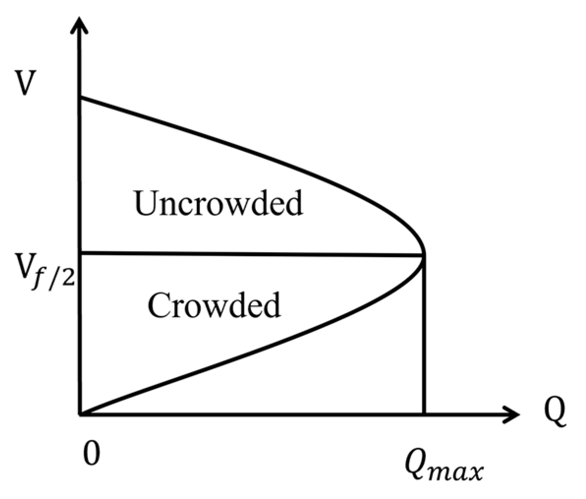
The speed-flow model parameter relationship is a functional model that describes the relationship between the speed of vehicles traveling on a road and the volume of traffic [29]. When the traffic flow on the road does not reach basic capacity, the vehicle operation state is uncongested, the speed increases, then the traffic flow increases, and the vehicle can travel at the desired speed. When the traffic flow on the road reaches the road capacity, the vehicle operation state is in a congested state, the vehicle operation speed will gradually decrease, the vehicle headway time distance will become larger and the time interval between two consecutive vehicles through the same section will increase. Therefore, the traffic flow will also gradually decrease until it decreases to zero. The speed-flow model for the full process state is shown in Figure 4.
In the free-flow condition, the speed-flow rate is linear. In the non-free-flow condition, the speed-flow rate is curvilinear. This can be verified by fitting the primary and quadratic functions, respectively [38]. Therefore, in this paper, for the speed-flow model in the congested state, the quadratic function v < v m was fitted, and for the speed-flow model in the uncongested state, the primary function v > v m was fitted. The functional relationship is shown in Equation (1).
v = { a Q 2 + b Q + C                                       v < v m a 1 + b 1 Q                                                         v > v m
where: v = speed (km/h);
  • Q = traffic volume (pcu/h);
  • v m = the speed corresponding to the maximum traffic capacity (km/h);
  • a , b , c , a 1 , = model parameters.
Firstly, the intersection velocity-flow model was fitted in Figure 5.
According to the fitting results in Figure 5, the intersection speed-flow function relationship Equation (2) was obtained.
v = { 4 × 10 6 Q 2 + 0.0086 Q + 11.339                                         v < v m 49.565 0.0075 Q                                                                                           v > v m
In the uncrowded and crowded states, the larger the R2 value is, the better the fit is. The model determination coefficients were all greater than 0.5, indicating that the function fits the observed values to an acceptable degree, and the error meets the requirements. According to Equation (2), it can be derived that Q = 1542 pcu/h when the maximum capacity = 38 km/h.
Secondly, the entrance and exit velocity-flow model was fitted in Figure 6.
According to the fitting results in Figure 6, the inlet/outlet speed-flow function Equation (3) is obtained.
v = { 5 × 10 6 Q + 0.0138 Q + 5.1403                           v < v m 45.739 0.0077 Q                                                                         v > v m
In the uncrowded and crowded states, the larger the R2 value is, the better the fit is. The model determination coefficients were all greater than 0.5, indicating that the function fits the observed values to an acceptable degree and the error meets the requirements. According to Equation (3), when Q = 1268 pcu/h, the traffic capacity is the maximum, and = 3 4 km/h.
By analyzing and studying the speed-flow curve model of traffic at entrances and exits and intersections, the maximum value of capacity and the expected value of speed can be derived according to the formula. These values provided basic data for the calibration of the parameters of the simulation experiments later, such as the upper limit of traffic volume, desired speed setting, etc.

2.2.2. Headway Time Distribution

Headway time distribution is an important component of traffic flow theory research. With the increase of road traffic load, there are several models for describing the corresponding law: negative exponential distribution, shifted negative exponential distribution, M3 distribution and other models. The negative exponential distribution and shifted negative exponential distribution are more suitable for low traffic volume. When traffic is heavy, the M3 distribution model is more suitable [39,40]. In this paper, the M3 distribution model is adopted because of the large vehicle flow at the intersection [41]. In this paper, 200 sets of observations at the inlet section of the intersection in Section 2.2.1 with a flow rate of 1512 pcu/h were selected for fitting the M3 distribution, as shown in Formula (4). A chi-square test was performed after calculating.
χ 2 = ( i = 0 14 f i F i 2 ) N = 18.76
Degree of freedom   D F = 15 1 = 14 , take α = 0.05.
Search the table to get α 2 = 23.68 > 18.76, the observed frequency and theoretical frequency fit is good, and it can be inferred that the headway time distance obeys the M3 distribution.
Some of the observed data in Section 2.2.1 when the entrance/exit is 512 pcu/h were selected for collation, and the critical gap of the headway time distance at the entrance/exit was determined by the maximum likelihood estimation method. Using this in combination with function distribution fitting, the headway time distance of the intersection was found to approximately obey the M3 Distribution, and the headway time distance can be considered 2.5 s. The insertable critical gap of the entrance/exit obeys the second-order Erlang Distribution, and the headway time distance for this can be considered 3.0 s.

2.2.3. Behavioral Analysis of Vehicle Lane Change

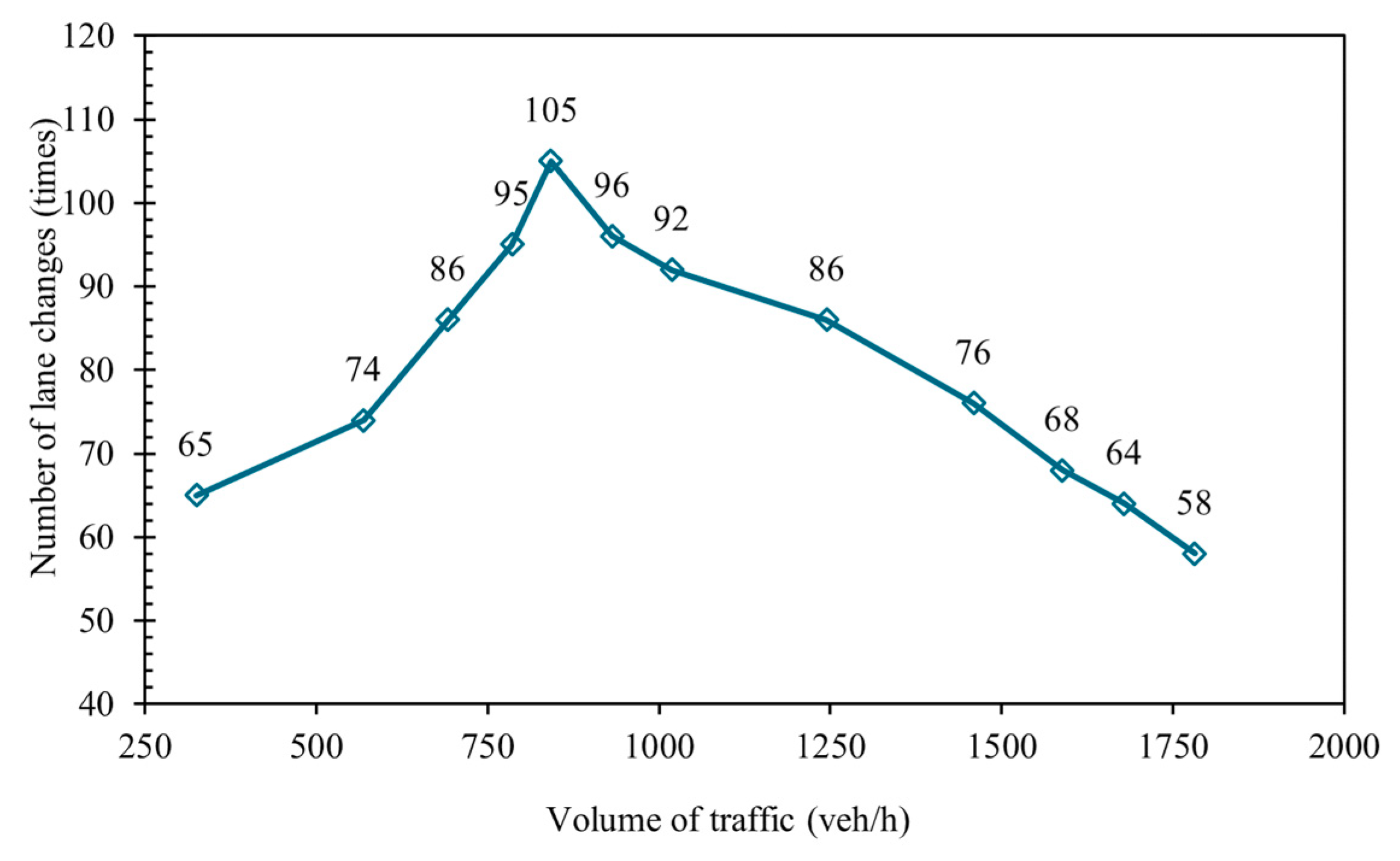
According to the analysis of the survey data, when the traffic volume on the city road is low, the driver can drive as he wishes at the desired speed, and the speed is relatively high. Most of the lane changes at this time are due to travel demand factors, so the number of lane changes is relatively small. When the traffic volume increases to a certain extent during the peak period, the speed may be restricted, and the number of lane changes gradually increases. When the traffic volume reaches saturation, the dispersion between vehicles is small. If there is a demand for a lane change, it is difficult to complete the lane change, so with the increase of traffic volume, the number of lane changes shows a trend of increase first and then decrease. The survey data are shown in Figure 7.
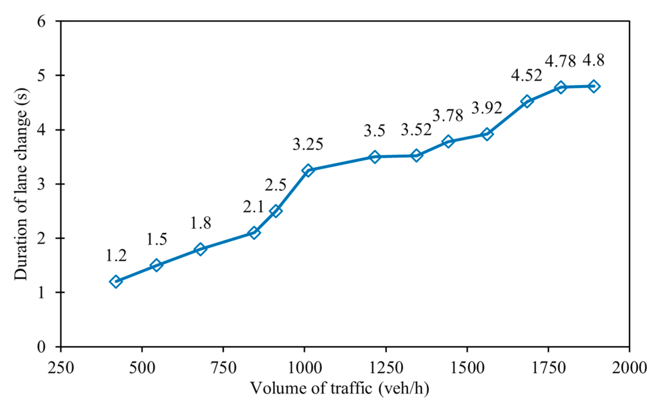
In different traffic volume conditions, due to various environmental factors, the vehicle lane change duration will be significantly different. Lane change duration will directly affect the distance of the vehicle movement. Survey data can quantitatively analyze the relationship between different traffic volumes and lane change duration. The survey data are shown in Figure 8.

3. Model Building and VISSIM Simulation

3.1. Model Building

3.1.1. Computational Models for Converging, Weaving and Queuing Sections

  • The length of the converging section L1 is shown in Equation (5):
L 1 = ( v 1 3.6 ) 2 ( v 2 3.6 ) 2 2 a
  • L 1 = length of converging section (m);
  • v 1 = the speed at which the vehicle is traveling when it first enters the converging section (km/h);
  • v 2 = speed at which the vehicle leaves the converging section (km/h);
  • a = vehicle acceleration, based on the analysis of traffic survey data in the previous paragraph, taking a fixed value of 1.5 m/s2.
b.
The length of the weaving section L2 is shown in Equation (6):
L 2 = L 21 + L 22 + L 23 + L 24
The length L2 of the weaving section can be further divided into four stages consisting of the following sections: the distance L21 needed for the vehicle to travel when the vehicle waited for an insertable gap, the distance L22 for the vehicle to judge and take measures to travel, the distance L23 for the vehicle to change to the target lane to travel and the distance L24 for the vehicle to slow down and line up to travel after completing the lane change.
According to the relevant research results, it was found that the traffic flow on the road obeys Poisson distribution, and the headway can be described by the shift negative exponential distribution curve [42]. The distribution function of the shifted negative exponential distribution is shown in Equation (7):
P ( h t ) = e λ ( t τ )
  • λ = average number of vehicles arriving (pcu/s);
  • τ = the minimum value of headway time distance, taking the value of 1.0 to 1.5 s.
The average waiting time for the vehicle waiting gap could be obtained through a series of mathematical equations in constant transformation with the Laplace variation, using the Markov property and boundary conditions of probability, which is shown in Equation (8):
t w = 1 λ [ e λ ( t c τ ) λ t c τ 1 ]
  • t w = average waiting time (s);
  • λ = average number of vehicles arriving (pcu/s);
  • τ = the minimum value of headway time distance, taking the value of 1.0 to 1.5 s;
  • t c = critical gap time, which was taken as 2.5 s, based on the analysis of the survey data.
Therefore, the expression L21 for the distance traveled while the vehicle is waiting for the insertable gap is Equation (9):
L 21 = v 3 3.6 t w
  • L 21 = distance traveled while the vehicle waits for an insertable gap (m);
  • v 3 = average speed of vehicles traveling in the weaving section (km/h);
  • t w = average vehicle waiting time at a given insertable gap (s).
The travel distance L22 of the vehicle judgment and measures is Equation (10):
L 22 = v 3 3.6 t 2
  • L 22 = judgment and distance of measures (m);
  • v 3 = average speed of vehicles traveling in the weaving section (km/h);
  • t 2 = average waiting time for a vehicle to find an insertable gap (s).
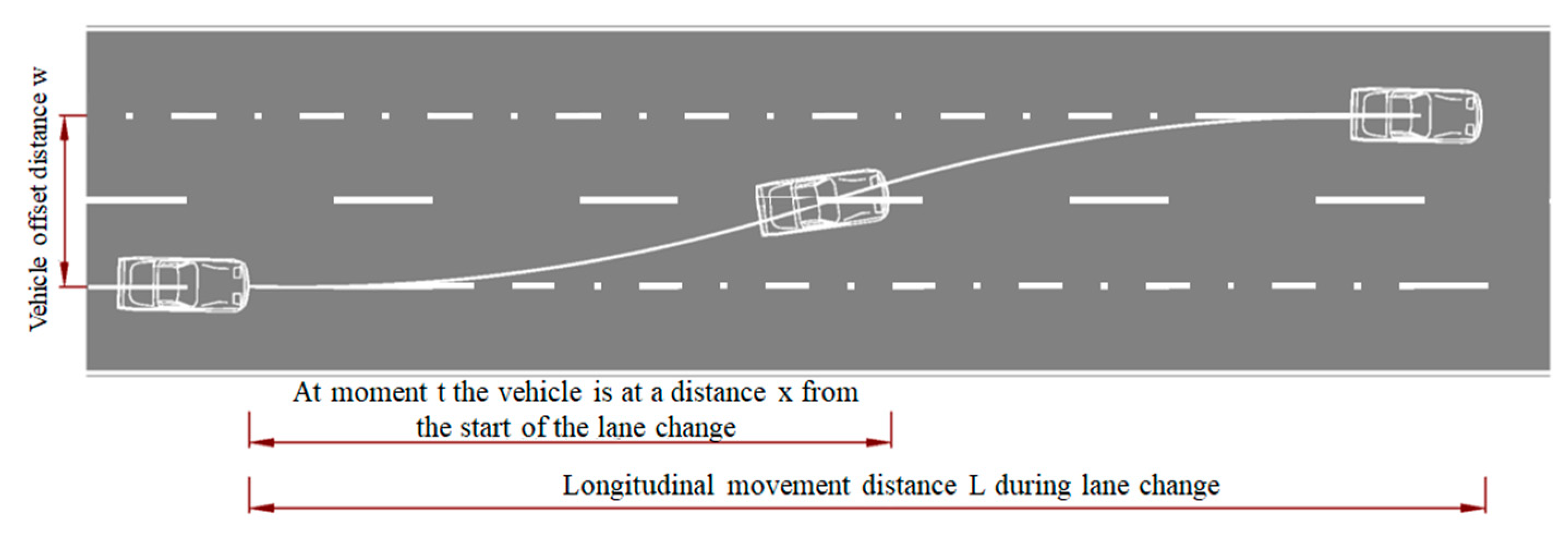
For the distance from the lane change to the target lane L23, it was shown that the vehicle lane change should satisfy two basic principles [43]. First, in the process of changing lanes, the curvature of the travel trajectory should change continuously, without sudden changes. Second, the curvature of the starting and ending points of the lane change trajectory was minimized to zero. Following the latest research results in China, this paper adopted the equal speed offset cosine curve lane change model, which can more accurately describe the whole process of actual vehicle lane change [44]. The expression of the model is shown in Equation (11):
y = W x L W 2 π c o s [ π L 2 ( x L 4 ) ] , x [ 0 , L ]
Equation (12) can be obtained by performing a constant mathematical transformation of Equation (11):
y = W 2 π × { π 2 + π L 2 ( x L 4 ) c o s [ π L 2 ( x L 4 ) ] } , x [ 0 , L ]
  • W = distance between the centerlines of two adjacent lanes (m);
  • L = longitudinal movement distance required for the vehicle to complete the lane change (m);
  • x = the distance travelled by the vehicle at moment t (m), i.e., d x = v 3 d t , v 3 is the running speed of the vehicle changing lanes (m/s).
The specific lane change trajectory is shown in Figure 9.
Deriving Equation (12) for time t yields Equation (13):
d y d t = W v 3 L { 1 + s i n [ π L 2 × ( x L 4 ) ] } d 2 y d t 2 = 2 π W ( v 3 L ) 2 c o s [ π L 2 × ( x L 4 ) ] d 3 y d t 3 = ( 2 π ) 2 W ( v 3 L ) 3 s i n [ π L 2 × ( x L 4 ) ]
  • W = distance between the centerlines of two adjacent lanes (m);
  • v 3 = average speed of vehicles traveling in the weaving section (km/h);
  • L = longitudinal movement distance required for the vehicle to complete the lane change (m).
In order to ensure the safety and stability of the vehicle during the lane change, Equations (14) and (15) must be satisfied at any moment t:
d 2 y d t 2 2 π W ( v 3 L ) 2 a m a x
d 3 y d t 3 ( 2 π ) 2 W ( v 3 L ) 3 α m a x
  • a m a x = maximum allowable lateral acceleration ( m s 2 );
  • α m a x = maximum allowable rate of change of lateral acceleration ( m s 3 ).
According to Equations (14) and (15), the lane transformation to the target lane length L 23 is obtained by satisfying Equation (16):
L 23 max ( 2 π W a m a x v 3 , ( 2 π ) 2 W α max 3 v 3 )
Then, the maximum fading rate K m a x of the lane transformation to the target lane section should satisfy Equation (17):
K m a x = W / m a x ( 2 π W a m a x v 3 , ( 2 π ) 2 W α m a x 3 v 3 )
Deceleration distance L24 after the vehicle completes lane change is shown in Equation (18):
L 24 = ( v 3 3.6 ) 2 ( v 4 3.6 ) 2 2 a
  • L 24 = deceleration distance (m);
  • v 4 = travel speed when vehicles slow down and queue (km/h);
  • a   = vehicle deceleration, based on the analysis of the previous survey data, is taken as 2.0 m/s2.
c.
Entrances/exits queue section length calculation model L3.
Queuing at entrances and exits can be thought of as a single-lane queuing service (M/M/1) system.
Therefore, the queue section length L3 is shown as Equation (19):
L 3 = N × ( l + d ) = ρ 2 1 ρ ( l + d ) = ( λ μ ) 2 1 ( λ μ ) ( l + d )
  • L 3 = length of queuing section (m);
  • λ = average arrival rate of vehicles (pcu/h);
  • μ = service rate of vehicles approaching the entrance/exit (pcu/h);
  • ρ = traffic intensity or the utilization coefficient;
  • l = average vehicle length (m);
  • d = reasonable clearance between vehicles (m).
d.
Intersection queue length calculation model L4.
Wave in traffic: assume that the vehicle volume coming from upstream is Q 1 and the red light time is tA, then the intersection inlet lane queue length is calculated as follows: let the flow of the convoy be Q 1 , the speed be v 1 and the density be k 1 , when a red light is encountered, at this time there is a gathering wave generated by stopping the convoy propagating from front to back. When the wave passes through later, the flow Q 2 = 0, v 2 = 0 and the density k 2 = k j . When encountering a green light, at this time there is a dissipation wave generated by the green light start in the convoy propagated from front to back, after the time t seconds, passing to a place in the queue, the queue length will no longer increase. At this time the traffic flow is Q 3 , the speed is v 3 and the density is k 3 .
The speed–density linear relationship model proposed by Greenshields [45] is shown as Equation (20):
v = v f ( 1 k k j )
Assuming that the traffic flow is uninterrupted, the basic model of traffic flow is valid, and Equation (21) is given:
Q = k v
According to Equations (20) and (21), Equations (22) and (23) can be obtained:
Q = v f ( k k 2 k j )
k i = 0.5 k j ( 1 - 1 Q i Q m )
  • Q = traffic Volume (pcu/h);
  • v = average vehicle speed (km/h);
  • v f = average speed of unobstructed vehicle traffic (km/h);
  • k = average traffic density (vehicle/km);
  • k j = traffic jam density (vehicle/km);
  • k i = the traffic density of the traffic in state i.
The wave flow of the gathering wave formed at the red light and the wave flow of the dissipating wave formed when the green light is on are expressed by the Equation (24):
Q W 1 = V 2 V 1 K j K 1 Q W 2 = V 2 V 3 K j K 3
  • Q W 1 , Q W 2 = wave flow of gathering and dissipating waves (pcu/h);
  • V 1 , V 2 , V 3 = speed before the red light, at the red light, and the green light (km/h);
  • K 1 , K 3 = traffic density before the red light and at the green light (pcu/km).
Duration of dissipation after green light activation is shown as Equation (25):
t s = Q W 1 × t A Q W 1 Q W 2
  • Q W 1 , Q W 2 = wave flow of gathering and dissipating waves (pcu/h);
  • t A = red Light Duration (s).
The queue section length L4 is shown as Equation (26):
L 4 = Q W 1 × ( t A + t s ) K j
  • L 4   = length of queueing section (m);
  • Q W 1 = aggregate wave flow (pcu/h);
  • K j = blocking density, the density when the traffic is so dense that vehicles cannot move (pcu/km);
  • t A = red Light Duration (s);
  • t s = dissipation duration (s).

3.1.2. Distance Calculation Model Entrances/Exits and Intersection

  • Distance model for signal-controlled entrances and exits to adjacent intersections.
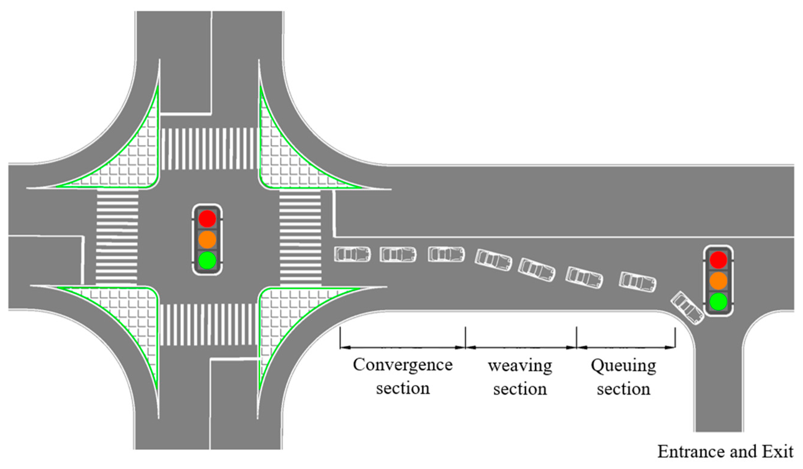
When the entrance and exit are located upstream of the intersection, the entrance and exit vehicles converge in the outer lane of the road, due to the large difference in speed with the mainline traffic flow, the vehicle driving in an unstable state and the vehicle in the outer lane accelerating to the same speed as the mainline. The length of the acceleration lane can be determined following the vehicle uniform acceleration to the mainline straight vehicle driving speed, and the travel distance is the length of the converging section. When a vehicle travels at a signal-controlled intersection, there are still vehicles ahead waiting at the stop, generating a queue section length, then the signal-controlled entrance/exit is located at the upstream distance combination of the intersection, as shown in Figure 10.
Therefore, the distance model for the signal-controlled entrances/exits located upstream of the intersection can be obtained as Equation (27):
L = L 1 + L 2 + L 4 = ( v 2 3.6 ) 2 ( v 1 3.6 ) 2 2 a + v 3 3.6 t w + v 3 3.6 t 2 + ( v 3 3.6 ) 2 ( v 4 3.6 ) 2 2 a + Q W 1 × ( t A + t s ) K j + m a x ( 2 π W a m a x v 3 , ( 2 π ) 2 W α m a x 3 v 3 )
The minimum distance between the signal-controlled entrance and exit upstream of the intersection is calculated according to the above model, as shown in Table 2.
When the entrance and exit are located downstream of the intersection, the vehicle driving through the intersection range drives into the exit road and into the connecting section. The speed of the vehicle at this time is different from that of the main line, and the vehicle is still in an unstable state. This paper used the convergence section length, which can be determined by following the uniform vehicle acceleration from the main road straight vehicle driving speed, and the driving distance is the convergence section length. Consider the most unfavorable conditions of vehicle travel, when the vehicle moves from the outermost lane to the inner lane, then the horizontal distance traveled is the length of the weaving section. When the vehicle travels to the entrance/exit with signal control, there are still vehicles in front of it waiting for parking, generating the length of the queuing section, and the signal control entrance/exit is located at the downstream distance combination of the intersection, as shown in Figure 11.
Therefore, based on the above analysis, the distance model for signal-controlled entrances and exits located downstream of the intersection can be derived as Equation (28):
L = L 1 + L 2 + L 3 = ( v 2 3.6 ) 2 ( v 1 3.6 ) 2 2 a + v 3 3.6 t w + v 3 3.6 t 2 + ( v 3 3.6 ) 2 ( v 4 3.6 ) 2 2 a + ( λ μ ) 2 1 ( λ μ ) ( l + d )   + m a x ( 2 π W a m a x v 3 , ( 2 π ) 2 W α m a x 3 v 3 )
The minimum distance between the signal-controlled entrance and exit located downstream of the intersection was calculated according to the above model, as shown in Table 3.
b.
Distance model for unsignalized entrances and exits to adjacent intersections.
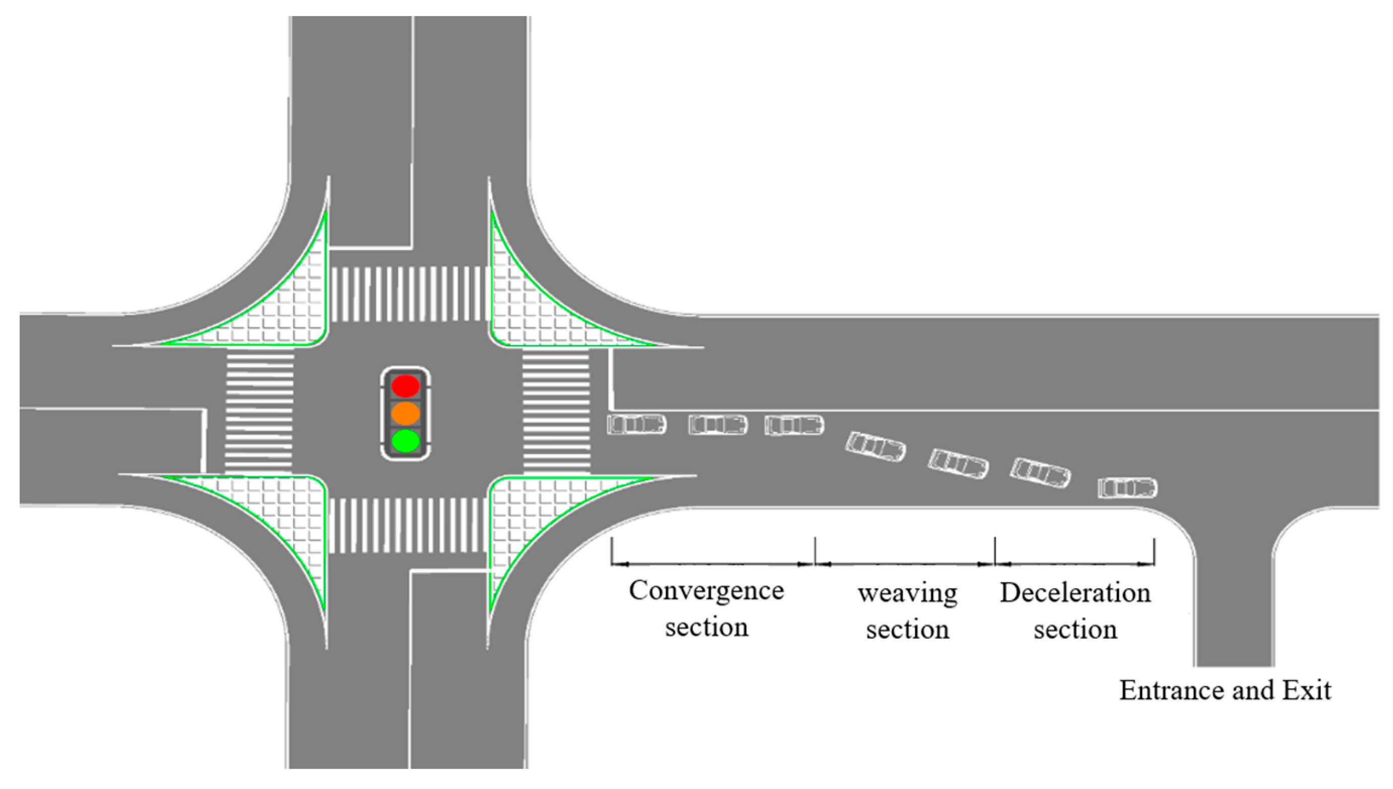
When the unsignalized control entrance/exit is located downstream of the intersection, as discussed in the first half of this subsection, the distance composition only needs to consider the length of the steady vehicle travel convergence section, the length of the weaving section and the length of the deceleration section. The queue length on the main road can be disregarded, since queues are less likely to occur at signal-less controlled entrances/exits within a reasonable distance. The minimum distance composition is shown in Figure 12.
As the vehicle tends to reach the entrance/exit, the speed will gradually decrease and travel slowly. According to the analysis of traffic flow characteristics, the final speed v 4 of vehicle deceleration is 20km/h. Therefore, the minimum distance model for unsignalized controlled entrances/exits located downstream of the intersection is as Equation (29), and the minimum distance value is shown in Table 4.
L = L 1 + L 2 = ( v 2 3.6 ) 2 ( v 1 3.6 ) 2 2 a + v 3 3.6 t w + v 3 3.6 t 2 + ( v 3 3.6 ) 2 ( v 4 3.6 ) 2 2 a + m a x ( 2 π W a m a x v 3 , ( 2 π ) 2 W α m a x 3 v 3 )
When the unsignalized control entrance/exit is located upstream of the intersection, the entrance/exit with or without signal control has less influence on the calculation of the distance model for the entrance/exit located upstream of the intersection studied in this paper, and the vehicle operation status is the same. Therefore, this subsection of the study is the same as the study of the convergence section length L1 in Section 3.1.1. The conclusion is the same, and the distance model of the unsignalized control entrance/exit located upstream of the intersection is shown in Equation (27), and the minimum distance value is shown in Table 2.
c.
Distance model for two adjacent entrances and exits.
Since the operation status of signal-controlled entrances and exits was relatively complex, the distance between two adjacent signal-controlled entrances and exits was selected for analysis. When the vehicles leaving the entrance/exit converge to the main road, they can drive straight along the outer lane to the adjacent entrance/exit without changing lanes. Only the length of the convergence section, the length of the deceleration section and the length of the queuing section need to be considered, and the distance combination is shown in Figure 13.
The minimum distance between two adjacent signal-controlled entrances and exits at different design speeds is obtained according to Equation (30):
L = L 1 + L 24 + L 3 = ( v 2 3.6 ) 2 ( v 1 3.6 ) 2 2 a + ( v 3 3.6 ) 2 ( v 4 3.6 ) 2 2 a + ( λ μ ) 2 1 ( λ μ ) ( l + d )
The minimum distance between two adjacent entrances and exits can be reached only by driving along a straight line, so the following table does not consider the minimum distance for the different number of lanes, as shown in Table 5.

3.2. VISSIM Simulation Parameter Calibration

Currently, VISSIM software is used for simulation evaluation of the studied object in domestic research, but the applicability of the model parameters is often ignored, leading to errors between the simulation results and actual situations. There are many model parameters in VISSIM, so in order to ensure the applicability of the simulation model, it is necessary to calibrate many simulation parameters in the model. In this paper, through the analysis of field survey data, measured data was selected to verify and calibrate simulation parameters.

3.2.1. Geometric Conditions of the Roadway

When conducting traffic simulation using VISSIM, the first step is to calibrate the parameters related to road conditions, entrances and exits and intersections. Based on the field traffic survey data in this paper, the parameter values are shown in Table 6.

3.2.2. Traffic Volume

Based on the traffic survey data, the traffic volume of each entrance at the intersection was analyzed, and the peak hourly traffic volume for the north entrance was 1227 pcu/h, while for the west entrance it was 1512 pcu/h. According to the established speed-flow model of the intersection, the maximum traffic volume was calculated to be 1542 pcu/h, and the upper limit was set at 1600 pcu/h, while the lower limit was set at 800 pcu/h.
According to the traffic survey data, the peak hourly traffic volume at the entrance and exit was 512 pcu/h, and the maximum traffic volume according to the established speed-flow model was calculated to be 1268 pcu/h. In this paper, the upper limit was set at the maximum flow value of 1300 pcu/h, and the lower limit was set at 500 pcu/h.
Based on the survey data, the VISSIM traffic volume related parameters can be set accordingly.

3.2.3. Signal Control

Based on the field survey data, the signal cycle time of the intersection under study was 120 s. Therefore, when simulating the signal control of the intersection, the signal timing was set based on the field survey data. The VISSIM signal timing is shown in Figure 14.

3.3. Simulation Results and Discussion

3.3.1. Simulation of Traffic with Entrances and Exits Located Upstream of Intersections

  • Cross-sectional traffic flow parameters.
Two parameters, vehicle speed and queuing delay, were chosen as the characteristic parameters of traffic flow at the cross-section to evaluate the simulation effects of the current length and the calculated length of the model.
The characteristic parameters of the cross-sectional traffic flow can be detected by setting data detection points. The data detection points should be set in lanes to be able to detect the data of each lane parameter. The vehicle speed and queuing delay between the current length and the model calculated length were obtained, and the data were organized. The resulting data are shown in Table 7.
According to the results obtained from the Table 7 simulation, the two evaluation indexes of vehicle speed and queuing delay in the traffic flow characteristics parameters of the cross-section of the actual current length and the theoretical model calculated length were compared, and the vehicle travel speed of the theoretical model calculated length was improved to a certain extent compared to the actual current length. Travel speed increased by 11.63%, 15.86%, 12.93%, 12.36% and 2.17%, and queuing delays were reduced by 45.35%, 29.22%, 36.09%, 21.98% and 18.48%, respectively. A comparative analysis showed a more significant improvement in both vehicle speed and queuing delays.
b.
Traffic flow characteristics of road sections.
Travel time (including waiting or stopping waiting time): the time spent between the vehicle traveling from the start of the detected section to the end. The travel times that can be detected and the number of vehicles that pass through the selected section during the travel time are shown in Table 8.
According to the results obtained from the Table 8 simulation, the travel time and vehicle number evaluation indexes in the traffic flow characteristics parameters of the road section were compared, and the number of vehicles driving through the road section within the average travel time derived from the theoretical model calculation length increases less, but the average travel time of vehicles of the theoretical model length decreases than the average travel time of vehicles of the actual status quo length. The trip time was reduced by 45.93%, 23.42% and 35.65%, and the number of vehicles increased by 18.42%, 10.13% and 41.96%, respectively. Through the comparative analysis, it can be concluded that there is a more obvious improvement effect on both the travel time and the number of vehicles.
In this paper, we used the delay data output from the travel time detector, the actual status quo length and the delay obtained after the simulation of the theoretical model calculation length, as shown in Table 9.
As can be seen in the results obtained from the Table 9 simulation, the actual status quo length and the delay time evaluation index of the model calculated length were compared, the theoretical model calculated length than the actual status quo length vehicle delay had been improved and the delay time was reduced by 62.20%, 25.73% and 41.43%. Through comparative analysis, it can be concluded that the delay time has a certain improvement effect.
c.
Queuing characteristic parameters.
The queue counter in VISSIM has characteristic parameters such as maximum queue length, average queue length and the number of stops of queuing vehicles. Queue length refers to the distance between the stop line from the signal intersection to the end of the upstream queuing vehicles, expressed in terms of the number of queuing vehicles. The average queue length was obtained from the simulation evaluation of the actual status quo length and the theoretical model calculation length, as shown in Table 10.
As can be seen in the results obtained from the Table 10 simulation, the average queue length evaluation indexes of the current situation length and the theoretical model calculated length were compared, and the average queue length derived from the theoretical model calculated length is shorter than the actual current situation length. The average queue lengths were reduced by 40.72%, 27.19% and 9.55%. Through comparative analysis, it can be concluded that the average queue length has a more obvious improvement effect.

3.3.2. Simulation of Traffic with Entrances and Exits Located Downstream of Intersections

  • Cross-sectional traffic flow parameters.
Two parameters, vehicle speed, and queuing delay, were chosen to evaluate the simulation effect of the current length and the calculated length of the model for the cross-sectional traffic flow characteristics where the entrance and exit were located downstream of the intersection.
The characteristic parameters of the cross-sectional traffic flow can be detected by setting data detection points. The data detection points should be set in lanes to be able to detect the data of each lane parameter. The vehicle speed and queuing delay between the actual status quo length and the theoretical model calculation length were obtained, and the data are collated, and the resulting data are shown in Table 11.
As can be seen in the results obtained from the Table 11 simulation, the two evaluation indexes of vehicle speed and queuing delay in the traffic flow characteristics parameters of the cross-section of the current situation length and the model calculated length were compared, and the vehicle speed of the theoretical model calculated length was significantly improved compared to the actual current situation length. Vehicle speed increases of 37.73%, 27.86%, 21.61%, 35.06%, 43.59% and 43.40%, and the queuing delay reductions of 38.69%, 50.00%, 26.10%, 22.59%, 41.46% and 9.18%, respectively. A comparative analysis showed a more significant improvement in both vehicle speed and queuing delays.
b.
Road section traffic flow characteristics parameters.
The trip times and number of vehicles are shown in Table 12.
The results obtained from the Table 12 simulation show the travel time and the number of vehicles, and the index was evaluated for comparison. After comparing the parameters of travel time and vehicle count, the theoretical model’s calculated length resulted in a significant increase in the number of vehicles passing through the west exit section, and a notable reduction in travel time for the exit direction. The trip time decreases were 18.92%, 36.40% and 21.93%, and the number of vehicles increased by 15.66%, 13.04% and 44.92%, respectively. Through comparative analysis, it can be concluded that there was a certain improvement in travel time and the number of vehicles.
The delay is shown in Table 13.
As can be seen in the results obtained from the Table 13 simulation, the delay time evaluation indexes of the actual status quo length and the model calculated length were compared, and the delay time derived from the theoretical model calculated length was reduced compared to the actual status quo length. The delays were reduced to 29.66%, 73.47% and 26.23%. A comparative analysis showed that there was a more significant improvement in delay time.
c.
Queuing characteristic parameters.
The average queue length was obtained from the simulation evaluation of the actual status quo length and the theoretical model calculation length, as shown in Table 14.
As can be seen in the results obtained from the Table 14 simulation, the average queue length evaluation index in the traffic flow characteristics parameters of the road section of the current situation length and the model calculated length were compared, and the average queue length derived from the theoretical model calculated length has a certain degree of reduction compared to the actual current situation length. The average queue lengths were reduced to 55.40%, 57.36% and 21.46%. Through comparative analysis, it can be concluded that the average queue length has a more significant improvement effect.
As can be seen from the simulation output values in Table 7, Table 8, Table 9, Table 10, Table 11, Table 12, Table 13 and Table 14, the indicators under the calculated length of the theoretical model are significantly improved compared with the current actual length. When the entrances and exits are located upstream of the intersection, compared with the indicators under the actual length, the speed under the calculated length increases by 10.99% on average, queue delay decreases by 30.22% on average, travel time decreases by 35.00% on average, vehicle number increases by 23.50% on average, delay time decreases by 43.12% on average and queue length decreases by 25.82% on average. When the entrances and exits are located downstream of the intersection, compared with the indicators under the actual length, the average speed under the calculated length increases by 34.88% on average, queue delay decreases by 31.34% on average, travel time decreases by 25.75% on average, vehicle number increases by 24.54% on average, delay time decreases by 43.12% on average and queue length decreases by 44.74% on average. In summary, these results show that the application of the model proposed in this paper to optimize the distance between the project entrances/exits and the intersection can effectively improve the vehicle speed, travel time, vehicle number, delay, queue length and other indicators at the entrance/exits and intersections, so as to improve the traffic condition and operational efficiency within the scope of its influence.

4. Conclusions

The reasonable setting of entrances and exits is beneficial to improve the safety and operational efficiency of entrances/exits and intersections. In this paper, the distance between entrances/exits and adjacent intersections was studied through a combination of actual traffic survey, traffic characteristics analysis and theoretical analysis. The main conclusions are as follows.
(1)
According to the collected traffic flow survey data, the speed-flow functions of intersections, entrances and exits under congested and uncongested conditions were derived. By using the functional relationship fitting and the maximum likelihood estimation method, it was verified that the headway time distance at intersections obeys the M3 distribution. The headway time distance at entrances and exits obeyed the second-order of Erlang Distribution. The relationship between different traffic volumes and the number of lane changes and the relationship between different traffic volumes and the duration of lane changes were derived from the statistical analysis.
(2)
Based on the isokinetic offset cosine curve function, queuing theory and traffic flow fluctuation theory, the calculation models of the vehicle interleaving section and queuing section were established. Based on the basic calculation models of the converging section, weaving section and queuing section, the distance models of entrances and exits located upstream and downstream of the intersection were obtained. Based on the results of the traffic flow characteristics analysis, the minimum distance model values were calculated, and the recommended values were derived.
(3)
Based on the survey data, the VISSIM simulation parameters were calibrated, the actual length of the simulation was compared with the length of the theoretical model calculation and the operation effect of the theoretical model calculation worth improving was obtained, which verified the applicability and significant effect of the theoretical model proposed in this paper.
Due to limited research conditions, this study only focuses on certain areas of Wuhan. Further in-depth research and analysis are necessary to determine whether the simulation results can be applied to other regions. In addition, this study only evaluates simulated scenarios in certain situations, and the simulation performance in other scenarios requires further research.

Author Contributions

Conceptualization, F.X.; methodology, W.X. and F.W.; software, F.X.; validation, X.Z.; formal analysis, Y.W.; data curation, W.X.; writing—original draft preparation, F.W.; writing—review and editing, X.Z. and Y.W.; project administration, F.X. and W.X. All authors have read and agreed to the published version of the manuscript.

Funding

This research was funded by the Hebei Provincial Department of Transportation, China, (No. (2018) 409# 201816).

Institutional Review Board Statement

Not applicable.

Informed Consent Statement

Not applicable.

Data Availability Statement

All data covered in this paper are available from the corresponding author upon request.

Conflicts of Interest

The authors declare no conflict of interest.

References

  1. Divisions, C.; Song, X. Thoughts and Suggestions on China’s Smart City Building. Bull. Chin. Acad. Sci. 2021, 35, 34–39. [Google Scholar]
  2. Wang, F.; Tan, C.; Li, M.; Gu, D.; Wang, H. Research on traffic design of urban vital streets. Sustainability 2022, 14, 6468. [Google Scholar] [CrossRef]
  3. Yangyang, X.U. Research on Urban Traffic Congestion Based on Dijkstra Improved Algorithm. Geospat. Inf. 2019, 17, 80–82+11. [Google Scholar]
  4. Hua, P.; Yan, L. Study on the Mechanism of Transportation Affecting Analysis and Evaluation in Motorization Era. Chin. Overseas Archit. 2014, 157, 77–79. [Google Scholar]
  5. Lin, Z. An Investigation on Traffic Organization of Urban Expressway and Its Relevance with Road Network—Taking the Construction and Reconstruction of South Second Ring Road in Fuzhou as an Example. Fujian Constr. Sci. Technol. 2019, 167, 18–20+38. [Google Scholar]
  6. Kong, J. Design Method of Intersections of Urban Trunk Roads with Auxiliary Roads. Urban Roads Bridges Flood Control 2019, 243, 42–44+9. [Google Scholar]
  7. Ghosh, B.; Basu, B.; O’Mahony, M. Wavelet-Bayesian Hierarchical Short-Term Traffic Volume Model for Non Critical Junctions. 2022. Available online: https://www.semanticscholar.org/paper/Wavelet-Bayesian-Hierarchical-Short-Term-Traffic-Ghosh-O%E2%80%99Mahony/a18aa9d46f854a5c3c8d9566482707d97626bdb2?p2df (accessed on 19 March 2023).
  8. Alkheder, R. Bayesian combined neural network for traffic volume short-term forecasting at adjacent intersections. Neural Comput. Appl. 2021, 33, 1785–1836. [Google Scholar] [CrossRef]
  9. Mahmoud, N.; Abdel-Aty, M.; Cai, Q.; Yuan, J. Predicting cycle-level traffic movements at signalized intersections using machine learning models. Transp. Res. Part C Emerg. Technol. 2021, 124, 102930. [Google Scholar] [CrossRef]
  10. Yin, R.; Song, X. Mitigation strategy of cascading failures in urban traffic congestion based on complex networks. Int. J. Mod. Phys. C 2023, 34, 1–20. [Google Scholar] [CrossRef]
  11. Wu, L.; Zhang, R.; Zhou, R.; Wu, D. An edge computing based data detection scheme for traffic light at intersections. Comput. Commun. 2021, 176, 91–98. [Google Scholar] [CrossRef]
  12. Sutarto, H.Y.; Maulida, M.; Joelianto, E.; Samsi, A. Queue length optimization of vehicles at road intersection using parabolic interpolation method. In Proceedings of the 2015 International Conference on Automation, Cognitive Science, Optics, Micro Electro-Mechanical System, and Information Technology (ICACOMIT), Beijing, China, 22–24 August 2015. [Google Scholar]
  13. Zhu, Y.; Zhao, Z.; He, J.; Wang, Y. Study on intersection traffic lights timing optimization system based on sparrow algorithm. In Proceedings of the 2021 International Conference on Communications, Information System and Computer Engineering (CISCE), Beijing, China, 14–16 May 2021. [Google Scholar]
  14. Thakkar, J.M.; Sharma, A.; Parekh, V.; Juremalani, J. Effect of Left Turning Vehicle on Queue Length & Delay at Signalized Intersection: A Case Study of Vrundavan Cross Road Vadodara. International Journal of Technical Innovation in Modern Engeering & Science (IJTIMES) 2021. Available online: https://www.researchgate.net/publication/354021402_EFFECT_OF_LEFT_TURNING_VEHICLE_ON_QUEUE_LENGTH_DELAY_AT_SIGNALIZED_INTERSECTION_A_CASE_STUDY_OF_VRUNDAVAN_CROSS_ROAD_VADODARA (accessed on 19 March 2023).
  15. Singh, D.; Ameen, T.; Ahmad, A. Analysis of delay and queue length variation at three-leg signalized intersection under mixed traffic condition. Innov. Infrastruct. Solut. 2021, 6, 125. [Google Scholar] [CrossRef]
  16. Comert, G.; Khan, Z.; Rahman, M.; Chowdhury, M. Grey models for short-term queue length predictions for adaptive traffic signal control. Expert Syst. Appl. 2021, 185, 115618. [Google Scholar] [CrossRef]
  17. Gao, Y.; Qu, Z.; Song, X.; Yun, Z.; Xia, Y. A novel relationship model between signal timing, queue length and travel speed. Phys. A Stat. Mech. Its Appl. 2021, 583, 126331. [Google Scholar] [CrossRef]
  18. Xing, Y.; Gao, Z.; Qu, Z.; Hu, H. Study on Vehicle Delay Based on the Vehicle Arriving Distribution at Entrance Lanes of Intersection. Procedia Eng. 2016, 137, 599–608. [Google Scholar] [CrossRef]
  19. Palumbo, A.C.; Ayoub, N.; Whiting, M.T. Vehicle Queue Length and Traffic Delay Measurement Using Sensor Data for Traffic Management in a Transportation Network. U.S. Patent No. 11,270,581, 8 March 2022. [Google Scholar]
  20. Ruskic, N. Estimation of left-turn capacity at the unsignalized intersection. Simul. Model. Pract. Theory Int. J. Fed. Eur. Simul. Soc. 2021, 106, 102170. [Google Scholar] [CrossRef]
  21. Zeng, J.; Qian, Y.; Li, J.; Zhang, Y.; Xu, D. Congestion and energy consumption of heterogeneous traffic flow mixed with intelligent connected vehicles and platoons. Phys. A Stat. Mech. Its Appl. 2023, 609, 128331. [Google Scholar] [CrossRef]
  22. Mallipaddi, V.; Anderson, M. Evaluating Safety of Type-A Weaving Sections Using Geometric and Traffic Operational Factors. Int. J. Stat. Probab. 2020, 9, 21. [Google Scholar] [CrossRef]
  23. Youjun, X.U. Simulation of the Reasonable Distance between the Entrance of Urban Expressway and Signalized Intersection; Computer and Communications; Beijing University of Technology: Beijing, China, 2008. [Google Scholar]
  24. Marczak, F.; Daamen, W.; Buisson, C. Empirical analysis of lane changing behavior at a freeway weaving section. Traffic Manag. 2016, 3, 139–151. [Google Scholar]
  25. Li, W.; Wang, W.; Li, T.; Li, D. Characteristics analyses of merges on freeway acceleration lane. Dongnan Daxue Xuebao/J. Southeast Univ. (Nat. Sci. Ed.) 2002, 32, 252–255. [Google Scholar]
  26. Ahmed, A.; Abbas, M.; Ali, M.S.; Dong, N. Modeling the Effect of Length of Weaving Sections on Traffic Conditions at Unconventional U-Turns. In Proceedings of the 99th Annual Meeting of Transportation Research Board, Washington, DC, USA, 13–17 January 2019. [Google Scholar]
  27. Huang, Y.; Luo, Q.; Xu, L. Dynamic path optimization method based on ant colony algorithm and group decision-making. In Proceedings of the IEEE 10th World Congress on Intelligent Control and Automation, Beijing, China, 6–8 July 2012; pp. 300–304. [Google Scholar]
  28. Gattis, J.L.; Chimka, J.R.; Evans, A. Access Spacing Based on Turning-Vehicle Acceleration. Transp. Res. Rec. 2017, 2618, 1–7. [Google Scholar] [CrossRef]
  29. Papayannoulis, V.N.; Gluck, J.; Feeney, K.; Levinson, H.S. Access Spacing and Traffic Safety; Transportation Research Circular. 2022. Available online: https://trid.trb.org/view/686630 (accessed on 19 March 2023).
  30. Chu, C.M.; Huynh, N.; Chowdhury, M.; Ogle, J.H.; Sarasua, W.A.; Davis, W.J. Impact of Minimum Driveway Spacing Policies on Safety Performance: An Integrated Traffic Micro-Simulation and Automated Conflict Analysis. Int. J. Transp. Sci. Technol. 2014, 3, 249–264. [Google Scholar]
  31. Jauregui, X.; Weidner, J.; Cheu, R.L. Locations and Length of Entrances and Exits of an Automated Truck Lane on a US Freeway. In Proceedings of the IEEE 2021 Smart City Symposium Prague (SCSP), Prague, Czech Republic, 26–27 May 2021; pp. 1–5. [Google Scholar]
  32. Zhao, J.; Ma, W. An Alternative Design for the Intersections With Limited Traffic Lanes and Queuing Space. IEEE Trans. Intell. Transp. Syst. 2021, 22, 1473–1483. [Google Scholar] [CrossRef]
  33. Zhong, S.; Wang, Z.; Wang, Q.; Liu, A.; Cui, J. Exploring the Spatially Heterogeneous Effects of Urban Built Environment on Road Travel Time Variability. J. Transp. Eng. Part A Syst. 2021, 147, 04020142. [Google Scholar] [CrossRef]
  34. Schultz, G.G.; Braley, K.T.; Boschert, T. Relationship between access management and other physical roadway characteristics and safety. J. Transp. Eng. 2010, 136, 141–148. [Google Scholar] [CrossRef]
  35. Williams, K.M.; Stover, V.G.; Dixon, K.K.; Demosthenes, P. Coordination. In Access Management Manual. 2014. Available online: https://www.semanticscholar.org/paper/Access-Management-Manual-Williams-Stover/56d9bd06ac988d11051eb4a0d9f1dd1b18e4994b (accessed on 19 March 2023).
  36. Jun, J. Understanding the variability of speed distributions under mixed traffic conditions caused by holiday traffic. Transp. Res. Part C Emerg. Technol. 2010, 18, 599–610. [Google Scholar] [CrossRef]
  37. Wang, F.; Gu, D.; Chen, A. Analysis of traffic operation characteristics and calculation model of the length of the connecting section between ramp and intersection. Sustainability 2022, 14, 629. [Google Scholar] [CrossRef]
  38. Wang, W.; Cui, L. Speed-flow Model and Traffic Capacity on Urban Arterial Roads. Commun. Stand. 2011, 3, 50–52. [Google Scholar]
  39. Cowan, R.J. Useful headway models. Transp. Res. 1975, 9, 371–375. [Google Scholar] [CrossRef]
  40. Yin, S.; Li, Z.; Zhang, Y.; Yao, D.; Su, Y.; Li, L. Headway distribution modeling with regard to traffic status. In Proceedings of the 2009 IEEE Intelligent Vehicles Symposium, Xi’an, China, 3–5 June 2009; pp. 1057–1062. [Google Scholar]
  41. Zhang, G.; Wang, Y.; Wei, H.; Chen, Y. Examining headway distribution models with urban freeway loop event data. Transp. Res. Rec. 2007, 1999, 141–149. [Google Scholar] [CrossRef]
  42. Mo, Z. Poisson Distribution Based Mathematic Model of Producing Vehicles in Microscopic Traffic Simulator. J. Wuhan Univ. Technol. 2003, 27, 73–76. [Google Scholar]
  43. Yang, J.; Wang, J.; Li, Q.; Wang, Z. Behavior Analysis and Modeling of Lane Change in Traffic Micro-simulation. J. Highw. Transp. Res. Dev. 2004, 21, 93–97. [Google Scholar]
  44. Pan, B.H.; Liu, B.; Zhou, H.Y.; Huo, Y.F.; Sheng-Quan, W.U.; Highway, S.O.; University, C. Design index of transition section of ramp lane number change. J. Chang’an Univ. (Nat. Ence Ed.) 2018, 38, 82–88. [Google Scholar]
  45. Jun, X.U.; Luo, S.L. A study of connectness for the highway network. China J. Highw. Transp. 2000, 13, 95. [Google Scholar]
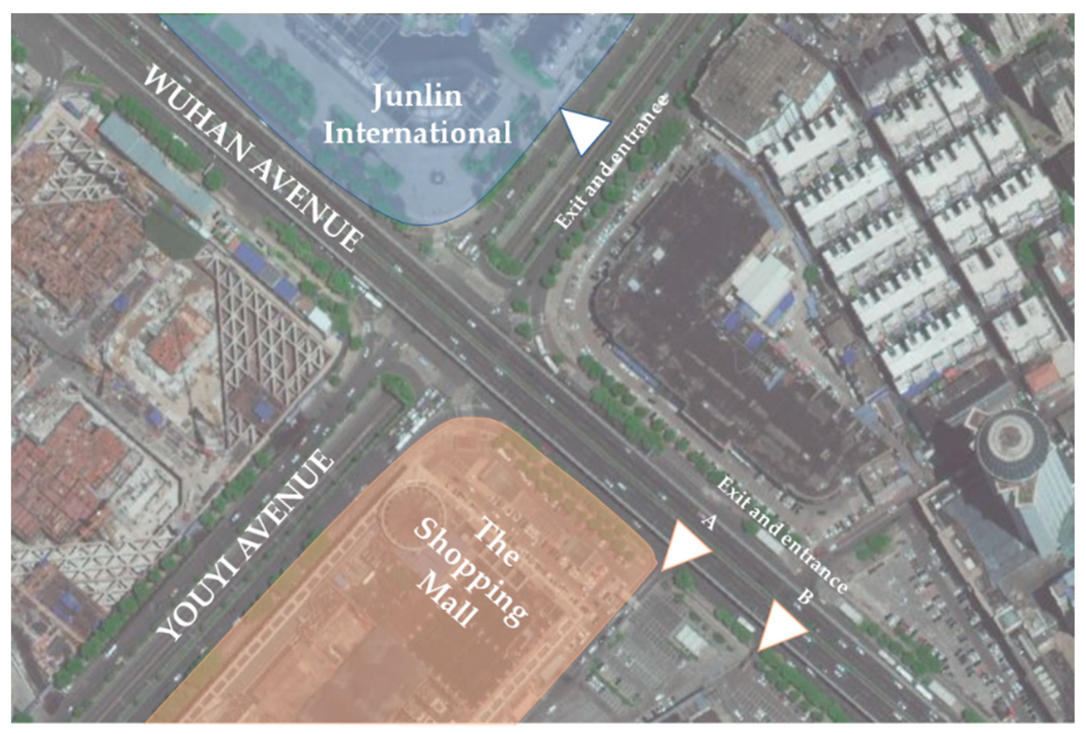
Figure 1. Map of the selected survey sites.
Sustainability 15 08656 g001
Figure 2. Traffic volume in and out during peak hours. (a) The entrance and exit of Junlin international; (b) exit and entrance of The Shopping Mall.
Sustainability 15 08656 g002
Figure 3. Section speed distribution. (a) Intersection entry; (b) intersection exit.
Sustainability 15 08656 g003
Figure 4. Actual speed-flow curve model diagram.
Sustainability 15 08656 g004
Figure 5. Intersection speed-flow curve model diagram.
Sustainability 15 08656 g005
Figure 6. Entrance and exit speed-flow curve model diagram.
Sustainability 15 08656 g006
Figure 7. Relationship between traffic volume and the number of lane changes.
Sustainability 15 08656 g007
Figure 8. Relationship between traffic volume and lane change duration.
Sustainability 15 08656 g008
Figure 9. Track diagram of vehicle lane change.
Sustainability 15 08656 g009
Figure 10. Combination of signal control entrances and exits at the upstream distance of the intersection.
Sustainability 15 08656 g010
Figure 11. Combination of signal control entrances and exits at the downstream distance of the intersection.
Sustainability 15 08656 g011
Figure 12. The combined distance of unsignalized entrances and exits located downstream of the intersection.
Sustainability 15 08656 g012
Figure 13. Combination of two adjacent entrance/exit spacing.
Sustainability 15 08656 g013
Figure 14. VISSIM signal timing diagram.
Sustainability 15 08656 g014
Table 1. Traffic volume at the intersection of Wuhan Avenue and Youyi Avenue.
TimeEast Entrance (pcu)South Entrance (pcu)West Entrance (pcu)North Entrance (pcu)
LSRLSRLSRLSR
17:00~17:15911266269835052293142013947
17:15~17:3010612247509139140351223215539
17:30~17:4512620457558941114284175216045
17:45~18:00142191755011156122324323514758
18:00~18:1510719442689950119320165921453
18:15~18:307419732588155161336235522556
18:30~18:4510022833536742119356213318339
18:45~19:009114941731033894290236521035
Table 2. Minimum distance from the signal-controlled entrance/exit upstream of the intersection.
Design Speed (km/h)Number of LanesModel Value (m)Recommended Value (m)
402154.45160
3179.62180
503207.31210
4232.82240
Table 3. Minimum distance from the signal-controlled entrance/exit at downstream of the intersection.
Design Speed (km/h)Number of LanesModel Value (m)Recommended Value (m)
402144.56150
3166.47170
503196.24200
4214.56220
Table 4. Minimum distance without signal control entrance/exit at the downstream of the intersection.
Design Speed (km/h)Number of LanesModel Value (m)Recommended Value (m)
402124.56130
3146.47150
503176.24180
4194.56200
Table 5. Minimum distance between two adjacent signal-controlled entrances and exits.
Design Speed (km/h)Model Value (m)Recommended Value (m)
40112.45120
50139.72140
Table 6. VISSIM basic road data.
ParameterParameter Value
Entrance lanes number at the intersection4
Entrance lanes number at the entrance/exit1
Width of main road lane3.75
Width of entrance lane at the entrance/exit3.5
Current length of entrance/exit located upstream of intersection (m) 76
Calculated length of the entrance/exit upstream of the intersection in the model (m) 200
Current length of entrance/exit located downstream of intersection (m)95
Calculated length of the entrance/exit downstream of the intersection in the model (m) 220
Table 7. Entrance/exit, intersection vehicle speed and queuing delay table.
TypeDirectionCurrent LengthModel Calculated Length
Vehicle SpeedQueuing DelayVehicle SpeedQueuing Delay
Entrance/ExitDrive in37.9316.1439.424.82
Drive out28.1029.2632.5820.71
Entrance RoadNorth left33.7169.1133.5744.17
North straight39.0154.2442.8342.32
North right46.0742.2047.0734.40
Table 8. Entrance/exit, intersection travel time and number of vehicles table.
TypeDirectionCurrent LengthModel Calculated Length
Travel Time(s)Vehicles NumberTravel Time(s)Vehicles Number
Entrance/ExitDrive in25.433813.7539
Drive out53.767941.1787
Entrance RoadNorth Entrance48.2711231.06159
Table 9. Entrance/exit and intersection delay schedule.
TypeDirectionCurrent LengthModel Calculated Length
Delay Time (s)Delay Time (s)
Entrance/ExitDrive in18.737.08
Drive out46.9434.86
Entrance RoadNorth Entrance41.4424.27
Table 10. Average queue length at entrances and intersections.
TypeDirectionCurrent LengthModel Calculated Length
Average Queue Length (m)Average Queue Length (m)
Entrance/ExitDrive in67.2239.85
Drive out85.9662.59
Entrance RoadNorth Entrance179.71162.54
Table 11. Entrance/exit, intersection vehicle speed and queuing delay table.
TypeDirectionCurrent LengthModel Calculated Length
Vehicle SpeedQueuing DelayVehicle SpeedQueuing Delay
Entrance/ExitDrive in18.1314.4524.978.86
Drive out25.560.2432.680.00
Entrance RoadWest Exit 137.1124.5245.1318.12
West Exit 231.2332.7242.1825.33
West Exit 329.2325.6941.9715.04
West Exit 426.8216.1338.4614.65
Table 12. Entrance/exit, intersection travel time and the number of vehicles table.
TypeDirectionCurrent LengthModel Calculated Length
Travel Time (s)Vehicles NumberTravel Time (s)Vehicles Number
Entrance/ExitDrive in20.568316.6796
Drive out12.94698.2378
Exit RoadWest Exit18.7923614.67342
Table 13. Entrance/exit, intersection delay schedule.
TypeDirectionCurrent LengthModel Calculated Length
Delay Time (s)Delay Time (s)
Entrance/ExitDrive in12.348.68
Drive out0.980.26
Exit RoadWest Exit11.828.72
Table 14. Average queue length table for entrances and exits, intersections.
TypeDirectionCurrent LengthModel Calculated Length
Average Queue Length (m)Average Queue Length (m)
Entrance/ExitDrive in27.7612.38
Drive out15.226.49
Exit RoadWest Exit85.9767.52
Disclaimer/Publisher’s Note: The statements, opinions and data contained in all publications are solely those of the individual author(s) and contributor(s) and not of MDPI and/or the editor(s). MDPI and/or the editor(s) disclaim responsibility for any injury to people or property resulting from any ideas, methods, instructions or products referred to in the content.