Abstract
Recently, solar energy has been gaining attention as one of the best promising renewable energy sources. Accurate PV power prediction models can solve the impact on the power system due to the non-linearity and randomness of PV power generation and play a crucial role in the operation and scheduling of power plants. This paper proposes a novel machine learning network framework to predict short-term PV power in a time-series manner. The combination of nonlinear auto-regressive neural networks with exogenous input (NARX), long short term memory (LSTM) neural network, and light gradient boosting machine (LightGBM) prediction model (NARX-LSTM-LightGBM) was constructed based on the combined modal decomposition. Specifically, this paper uses a dataset that includes ambient temperature, irradiance, inverter temperature, module temperature, etc. Firstly, the feature variables with high correlation effects on PV power were selected by Pearson correlation analysis. Furthermore, the PV power is decomposed into a new feature matrix by (EMD), (EEMD) and (CEEMDAN), i.e., the combination decomposition (CD), which deeply explores the intrinsic connection of PV power historical series information and reduces the non-smoothness of PV power. Finally, preliminary PV power prediction values and error correction vector are obtained by NARX prediction. Both are embedded into the NARX-LSTM-LightGBM model pair for PV power prediction, and then the error inverse method is used for weighted optimization to improve the accuracy of the PV power prediction. The experiments were conducted with the measured data from Andre Agassi College, USA, and the root mean square error (RMSE), mean absolute error (MAE), and mean absolute percentage error (MAPE) of the model under different weather conditions were lower than 1.665 kw, 0.892 kw and 0.211, respectively, which are better than the prediction results of other models and proved the effectiveness of the model.
1. Introduction
Solar power generation is safe and reliable and will not be affected by the energy crisis and fuel market instability factors. Photovoltaic power generation is one of the most important forms of solar power generation among many renewable energy sources because of its unique cleanliness, low cost, high efficiency, abundant reserves and low maintenance. Moreover, solar energy is the main renewable distributed energy source used to generate electricity worldwide. Italy reports that grid-connected electricity generation through solar PV power generation is 10 GW, the highest in the world. Thus, whether from the perspective of protecting the Earth’s environment or from the perspective of the sustainable development of the Earth’s resources, the future of photovoltaic power generation’s installed capacity will see significant growth. With the advancement of science and technology in recent years, PV power generation is growing quickly and accounting for an increasing share of power generation. PV systems play an important role, particularly in remote locations with large-scale PV power plants and residential power systems in rural areas [1,2,3,4].
However, solar PV power generation depends on its input, which is essentially stochastic and depends on the solar irradiation intensity. PV electricity output ceases when the sun sets and the solar panels are not illuminated. Even during the day, the output of photovoltaic power can fluctuate greatly due to cloudy and rainy weather. PV grid-connection has a substantial impact on the power system, therefore, in order to better utilize solar energy and vigorously develop PV power generation, accurate and reliable PV power prediction is necessary for power dispatch and allocation [5,6,7,8,9].
At present, there are several techniques for forecasting PV power, which is broadly categorized as conventional techniques and artificial-intelligence-based algorithms. Physical prediction techniques and time series prediction techniques are the two main traditional methodologies. The early stages of PV power prediction have seen the extensive use of the time series prediction method, but it has lower prediction accuracy [10,11]. Traditional machine learning models, such as random forest (RF) [12] and support vector machine (SVM) [13,14], which have higher prediction accuracy, are primarily used in applications of artificial intelligence algorithms. Neural networks are gradually becoming more popular in the field of PV prediction as deep learning advances. Numerous studies and experiments on the prediction of PV power by academics have demonstrated that combined prediction models typically produce better prediction outcomes than individual models. Additionally, it can help when an individual prediction model method produces large prediction errors at specific points. In [15], PV power was predicted with relatively high accuracy by recurrent neural network (RNN) model training on historical time series data. However, the gradient disappearance and gradient explosion limit the prediction time range. In addition, the RNN is under a high computational burden in the training phase as it needs a complete database for training, and if the quality of the data is poor, it will have a great impact on the prediction accuracy [16]. It is important to choose a model with strong performance. LSTM is widely used in processing problems for longer time sequences to overcome information loss, which is a good solution to the problem of gradient in RNN models [17,18,19]. In [20], the authors demonstrate that LSTM improves significantly in prediction accuracy compared to RNN, with lower error RMSE and MAE than other models. The back propagation (BP) neural network technique with time-delayed inputs serves as the foundation for the NARX neural network. The NARX neural network may successfully relate complicated dynamic interactions and react more swiftly to past state information by enhancing the time-delayed feedback connection from output to input. NARX has been used to resolve non-linear series forecasting issues in several disciplines and is appropriate for time series forecasting [21,22]. In [23], the authors proposed an RNN (DA-RNN). The concept of the DA-RNN mechanism is to use NARX to attend to the input sequence, followed by an LSTM to investigate the temporal instances. However, NARX may miss the interpretation of parts of the first-level attention under non-smooth weather conditions. In addition, the continuous computation of the pre-weighted inputs obtained from the encoder leads to a large computational effort. Although deep learning models can learn quickly and predict better outcomes, their structure is typically complex and computationally time-consuming, which results in low efficiency. An established and popular integrated learning strategy is the gradient boosting machine (GBM). extreme gradient boosting (XGBoost) is a gradient boosting tool that is incredibly scalable, adaptable, and versatile. XGBoost employs regularization to control the overfitting issue to efficiently utilize resources and get around the drawbacks of earlier gradient boosting algorithms [24]. In [25], the authors convert the weather feature vector into a Gram matrix, fully exploiting the intrinsic connection of the data, and using the particle swarm optimization algorithm to find the optimal hyperparameters of XGBoost to complete the PV power prediction; however, it has been concluded that XGBoost is time consuming in model training, leading to high memory usage and computational cost [26]. In comparison to XGBoost, LightGBM can speed up model training, uses less memory, allows for parallelized learning, and analyzes massive amounts of data without compromising accuracy [27,28,29]. In [26], the authors propose the use of LightGBM to predict PV power and show that it completes the training in a much shorter time (1.39 s) compared to 16.83 s for XGboost, with similar accuracy. The accuracy of the combined model prediction outputs can be increased by giving various models varied weights. Using different weights for each time point of various forecasting models, also known as variable weight combination forecasting [30] or weighting the forecasts of two models using the inverse of error method [31], can both improve accuracy, and the choice of weights is a crucial issue in these studies. All of the aforementioned literature provide direct predictions of the starting PV power, but because of the complicated nonlinear and stochastic nature of the meteorological elements affecting PV power, it is challenging to produce precise forecasts using the initial PV power.
To increase prediction accuracy, modal decomposition techniques and machine learning models can delve deeper into the latent hidden information in the data. Wavelet analysis and empirical mode decomposition are two frequently employed techniques. Both methods can decompose the original signal and can improve the prediction accuracy; however, they both have drawbacks. Wavelet analysis is poorly adapted, and EMD has problems, such as mode aliasing and over-envelope effects [32,33]. In [33], the PV power is decomposed by EMD, and the LSTM neural network is built for each intrinsic mode function (IMF) sequence to predict the PV power separately, and finally, the sub-series prediction results are superimposed to obtain the final prediction results; however, the prediction accuracy is limited due to the low correlation between the IMF of a part of the modal aliasing problem, and the sampling frequency of once an hour is not fine-grained enough. The purpose of EEMD [34] is to effectively improve the modal aliasing problem by introducing Gaussian white noise of equal amplitude to smooth the distribution of extreme points. However, the presence of noise signals of a certain amplitude in the decomposition component will affect the IMF quality leading to the degradation of prediction accuracy. CEEMDAN is created by enhancing the algorithmic method for EMD, which incorporates the benefits of both EEMD and EMD while also speeding up the decomposition process [35,36,37]. In [36], a prediction framework that combines a gated recurrent unit (GRU) with CEEMADAN is proposed. All of the above literature demonstrates the effectiveness of modal decomposition in PV power prediction; however, most studies have used a single machine learning model, and the generalizability and reliability of these studies remain inadequate. Combinatorial approaches in machine learning are often used to deal with the shortcomings of individual machine learning models as well.
In response to the above questions, the objective of the paper is to propose a new short-term prediction approach that is a combinatorial machine learning prediction model with CD. The performance of the proposed model is proven to be better than other models under different weather types. The main contributions of this paper can be summarized as follows:
- The decomposition of PV power by a combination of EMD, EEMD, and CEEMDAN was integrated with Pearson correlation analysis. The filtered high correlation IMF features substantially increase the accuracy of the model for PV power prediction;
- Preliminary NARX predictions and error correction vector features with high correlation coefficients are added to the NARX-LSTM-LightGBM. This enhanced the ability to parse PV data and the predictive performance of the proposed model in capturing actual PV power trends. Moreover, the models are combined by the inverse of error method, which greatly corrects the accuracy in case of large errors in individual models;
- A novel model for PV power prediction is analyzed in depth. The new approach is evaluated using a real dataset. A comparative study of the model performance under six test days (three types of weather) has been performed to reveal the high reliability of the proposed CD-NARX-LSTM-LightGBM model as a competitive model in capturing the time dependence with high accuracy.
2. PV Power Prediction Model Framework
2.1. Method of the Optimal Weight Determination
Features such as ambient temperature, PV inverter temperature, PV model temperature, solar irradiance, and wind speed influence PV power generation. To avoid the negative impacts of individual features on PV power prediction, the correlation coefficient of each feature variable regarding PV power is calculated using the Pearson correlation coefficient approach. With the following formula, the Pearson correlation coefficient evaluates the linear connection between two continuous variables [38,39,40]:
where is the mean value of the characteristic variable , and is the mean value of the characteristic variable y.
2.2. Modal Decomposition
For the non-stationary nature of PV power signals, it is necessary to construct the modal decomposition method without a parameter. EMD was recommended by NE. Huang et al. has a method for dissecting and examining nonlinear or non-stationary time series data. The advantage is that the signal is decomposed over the initial time scale of the data, using adaptively created intrinsic modal functions rather than fixed basis functions. EEMD is based on the EMD algorithm, which adds normally distributed white noise to the original signal so that the signal is uniformly distributed throughout the frequency band at the interval of extreme points, which effectively reduces the modal aliasing problem. CEEMADAN is an optimization algorithm based on EMD as well as the EEMD algorithm. The CEEMDAN algorithm enhances the speed of signal decomposition by adding a small amount of adaptive white noise to the EEMD algorithm. This fixes issues with the EEMD algorithm’s incompleteness and reconstruction error after adding white noise. The implementation steps of decomposition are listed as follows [41,42,43]:
- Adding white noise with a standard normal distribution to the raw signal. s(t). The i-th signal is denoted as , i = 1, 2… EMD decomposes the timing signal to obtain the corresponding sequence and the residual error vector :
- Adaptive white noise is added to the error, and the experiments are performed i times. Each time, the results are decomposed using EMD to obtain its first-order component . An error of the 2nd sequence removed from the 2nd sequence for CEEMDAN decomposition:
- To acquire the components that satisfy the conditions and the corresponding errors, the decomposition procedure is repeated. The repetition comes to an end if the error is a monotonic function and cannot be broken down by EMD. The original signal can be expressed as:
2.3. NARX Neural Network
NARX is a recurrent dynamic neural network. It has feedback connections that enclose several layers of the network, and it incorporates two time-delay structures from the signals at the input and output to describe the model of a nonlinear discrete system. The parametric formulas for the NARX neural network are as follows [44,45]:
where and denote the input and output values of the NARX neural network at the discrete moment n, respectively, and and , when greater than or equal to 0, are the maximum delay order of the input and output, respectively.
NARX’s feedback loop and delay mechanism improve the ability to retain historical time series data, which enables better exploration of the non-linear sequence relationships of time series data. The construction of the NARX neural network is shown in Figure 1.
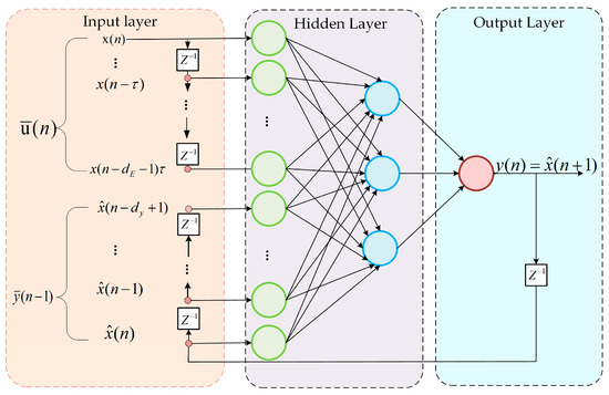
Figure 1.
NARX neural network structure diagram.
The NARX neural network has two layers of feedforward networks with a linear transfer function in the output layer and the hidden layer having a sigmoid function , calculated as:
The network has a time-delay structure to store sequential prior values of and , and the output is fed back to the input of the network. The input vectors are inserted through two-time delay structures of the input and output signals that demonstrate over-jump connections in the time-expanded network, increasing the capacity of the gradient descent to propagate back with shorter paths. This increases the NARX neural network’s capacity for historical data analysis [46].
2.4. Long Short-Term Memory
One of the major disadvantages of traditional neural networks is that they are not able to relate the current prediction results to historical time series data well in modeling. RNN introduces the concept of time series and improves this problem by iterating through the cycle, but it is difficult to train when the data is large because there is no forgetting mechanism that causes the gradient to explode or disappear. For the gradient problem, LSTM can be a useful solution. Through its special gate control and memory system, the LSTM neural network can fully use time series data [47,48]. The structure of the LSTM neural network is shown in Figure 2.
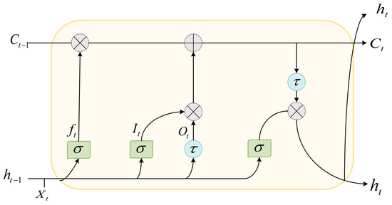
Figure 2.
LSTM neural network structure.
The LSTM mitigates the gradient explosion and gradient disappearance problems of the RNN through three gating structures, including the input gate , forget gate , and output gate . These gates are responsible for managing the interaction between memory cells implemented through tanh functions, sigmoid functions, and matrix multiplication. In addition, the forgetting gate has the ability to remove irrelevant states that mislead the prediction process, keeping only the important information to be forwarded to the hidden layer. The value of the forgetting gate ranges from 0 to 1, where a higher value means that the information is the most important to select for retention, and a result of 0 requires complete discard [49].
Here, contrary to the input gate, the output gate checks its effect on the state of other memory cells. The LSTM gates, hidden outputs, and cell states are given as follows [50]:
where and denote the input and storage units at time t, respectively. , , and are the deviation, cycle weight, and input weight of each gate, respectively. is the hidden layer of each gate at the moment of t − 1. The flow of the LSTM neural network operation is shown in Figure 2. Firstly, , , and input information to the LSTM cell. The LSTM gates interact with the input to generate a logic function. The input goes through , and a new cell state is constructed, quantifying the importance of the input information with 0 and 1 to be used to decide whether the input information is stored or not. Then, will update the cell state with the new important information. Finally, the remaining state values are calculated by the hidden layer of the LSTM.
2.5. LightGBM
The LightGBM base learner is a decision tree, which supports efficient parallel training. The advantages of LightGBM include faster training, lower memory consumption, better accuracy, and distributed support for the fast processing of large amounts of data. The decision tree algorithm by histogram, which obtains the leaf histogram by subtracting its father node histogram from its sibling node histogram, can be doubled in computational speed. To calculate the information gain, the LightGBM algorithm employs gradient-based one side sampling (GOSS), which not only reduces the number of samples used but also speeds up computation. Only the data with higher gradients are kept, while the data with smaller gradients are discarded. Exclusive feature bundling (EFB) makes several mutually exclusive features bind together, which can achieve the effect of reducing the data dimension [51]. The LightGBM algorithm effectively improves the operational efficiency through the leaf-wise growth strategy with depth limitation. It solves the problem that most GBDT tools use the inefficient level-wise decision tree growth strategy, which reduces the efficiency of machine learning by continuing to split and explore when the split gain is not high and achieves higher accuracy when the number of splits is the same [52].
2.6. Combined Forecasting Model and Process
The proposed model in this paper is a powerful combination of NARX, LSTM, and LightGBM models. The NARX-LSTM-LightGBM model merges the properties of each prediction model to obtain better results. In the proposed model, NARX is associated with the embedded memory that makes jump connections in the network. NARX is applied to calculate the error correction vector, which is utilized to reduce the dependence and sensitivity of the network structure on the time series. Let be the error vector between the actual value and the predicted value of NARX. The residuals are calculated as follows:
where and denote the nonlinear mapping function of the NARX and the corresponding weight values. Firstly, the initial PV power prediction from NARX is used to obtain the error correction vector. Then, the error correction vector and predictions are used as input for the new features. Finally, the LSTM and NARX predict the PV power with the data incorporating the new features as input, respectively. The NARX-LSTM model predictions are obtained by the integration of the two models through the inverse of error method. The formula is as follows:
where is the error of model 1 and is the error of model 2; w1 is the weight of model 1 and is the weight of model 2; and are the predicted values of model 1 and model 2, respectively; and is the error inverse method weighted average model.
Since NARX-LSTM is a combined model of deep learning and the LightGBM is a boosted tree machine learning model with a low correlation between the model principles, LightGBM has achieved better results in the field of prediction, so it combines the two. To obtain the final prediction results, the prediction results of the LightGBM algorithm and the combined NARX-LSTM algorithm are combined using the error inverse method. To better understand the proposed model, the combined prediction model is shown in Figure 3.
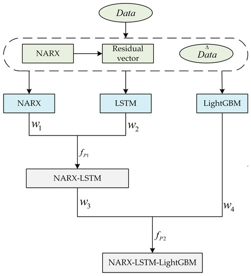
Figure 3.
Structure of combined prediction network.
Where and are the weights of the NARX neural network and the LSTM neural network, respectively; and are the weights of the combined NARX-LSTM model and the LightGBM algorithm, respectively. is the segmented data set. is the error inverse method weighted average model of NARX and LSTM; is the error inverse method weighted average model of combined NARX-LSTM and LightGBM.
To further enhance the exploration of the internal linkage of the historical time series, a prediction method based on the combined modal decomposition is proposed, and the flow chart is shown in Figure 4, which mainly consists of the following parts:
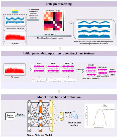
Figure 4.
Prediction flow chart.
- After pre-processing the data, only the data in the period of 5:00–20:00 retains. The Pearson algorithm analyzes the correlation of environmental features, selects the environmental variables with strong correlation as the features of the combined prediction model, and normalizes the features with strong correlation to improve the convergence speed and efficiency of the model.
- The EMD, EEMD, and CEEMDAN modal decomposition methods were selected to decompose the original PV power, and the respective modal sequence was combined to construct the feature matrix for correlation analysis, and the sequence features with high correlation and environmental features with strong correlation were selected to integrate into the NARX-LSTM-LightGBM prediction model.
- The proposed model predicts three typical types of weather (six test days) and evaluates the performance of NARX-LSTM-LightGBM.
2.7. Model Performance Evaluation Indicators
The indicators used in this paper to predict the selected performance evaluation include the MAE, the mean absolute percentage error (MAPE), and the root mean square error (RMSE). These percentage error measures are used because of their independent judgment and the efficiency of the judgment model. The formulas are as follows [53]:
where and are the actual and predicted values; is the sample mean.
3. Results and Discussions
3.1. Data Preprocessing
The performance of the proposed model was evaluated using real data sets, and the experimental study used measured data from Andre Agassi College, USA, to verify the generalization capability of the proposed model. The data set includes seven environmental characteristic variables: ambient temperature, PV inverter temperature, module temperature, irradiance, ambient humidity, wind speed, and wind direction.
The period of the dataset is 1 January 2012–31 December 2014, with a time interval of 15 min and a total of 96 sampling points a day. The time point of a day without PV power is eliminated to increase the efficiency of the model calculation, while the daily period of 5:00–20:00 with a time interval of 15 min and a total of 60 sampling points per day are kept. Missing data are filled by the mean fill method, and min–max normalization is done for the filled data.
3.2. PV Power Characteristics Correlation Analysis
The correlation of the characteristic variables has considerable significance to the accuracy of PV power prediction. In this paper, Table 1 [54] is used to define the degree of correlation between each environmental characteristic variable and PV power, and the Pearson correlation coefficients of the relevant environmental characteristic variables in the dataset for PV power are calculated by Equation (1) as shown in Table 2, the relative humidity and wind direction are not correlated, which are unfavorable to PV power prediction and therefore are discarded, and the wind speed is weakly correlated with less correlation to PV power, which is also negligible. Thus, we choose the strongly correlated environmental variables as the characteristic variables for prediction, i.e., ambient temperature, PV inverter temperature, PV panel temperature, and irradiance as the characteristic variables for the PV prediction model.

Table 1.
Correlation value thresholds.
Table 2.
Relative coefficients of power and individual characteristics.
3.3. Combinatorial Decomposition to Build New Features
This paper decomposes the original power using EMD, EEMD, and CEEMDAN decomposition methods to reduce the model’s complexity, thoroughly excavate the intrinsic information, and obtain 45 sequences to construct the feature matrix. The decomposed results are illustrated in Figure 5, Figure 6 and Figure 7. For example, in EEMD decomposition, IMF1–IMF9 are high-frequency sequences where the non-smooth data are concentrated, IMF10–IMF12 are medium-frequency sequences that vary with a certain period, and IMF13–IMF16 are low-frequency components with a larger period, which have little impact on the overall data fluctuations. From the figure, it can be known that the sequence after modal decomposition is simpler and smoother compared to the original PV power. Next, the decomposed sequences are analyzed for correlation to form a new feature matrix.
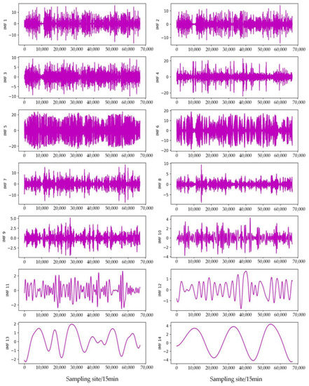
Figure 5.
Decomposition results of the PV series using EMD.
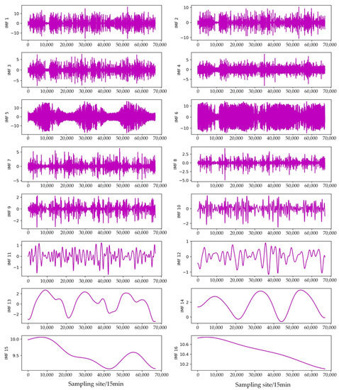
Figure 6.
Decomposition results of the PV series using EEMD.
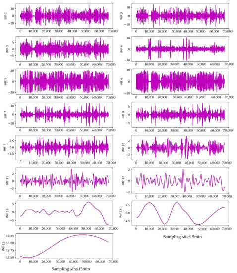
Figure 7.
Decomposition results of the PV series using CEEMDAN.
Too many sequences will result in low computational efficiency of the combined model, and non-correlated sequences will affect the prediction accuracy of the model, so the correlation analysis leaves a higher correlation with the PV power feature sequences to obtain the feature matrix. This paper selects the sequence with a correlation greater than 0.4 and combines them into a feature matrix. It is known from Table 3 that the correlation of the IMF5 sequence of EMD is 0.802; the correlation of IMF4, IMF5, and IMF6 sequence of EEMD are 0.614, 0.925, and 0.474, respectively; the correlation of IMF5 and IMF6 sequence of CEEMDAN are 0.684 and 0.574, respectively. Thus, these sequences are selected to form the new feature matrix and the rest of the sequence are excluded from the model.
Table 3.
The contrast of sequence correlations of different decomposition methods.
3.4. Model Parameters Setting
After several experiments, the prediction model was created by dividing the initial 66,870 sets of data into a training set and a test set in a ratio of 7:3, then feeding the results into a NARX neural network model with 12 hidden layer neurons and the order of the time delay being 8. The output 20,059 PV power test set and residual vector are obtained, and the latter 20,059 sets of the original data are jointly input into the LSTM neural network and LightGBM algorithm, and the correlation analysis shows that the test set power and residual vector have a high correlation of 0.87 and 0.51. The LSTM neural network model uses the ReLU function as the activation function, the optimizer is Adam, batch_size is 32, the maximum number of iterations is 32, and the learning rate is 0.1; the optimization of the LightGBM algorithm hyperparameters is performed using the grid search algorithm to obtain a learning rate of 0.01, the number of base learners (n_estimators) is 15,000, and the number of leaf nodes (num_leaves) is 31 by default.
Using the data from 6 February 2014 to 17 December 2014 as training samples, the PV power is shown in Figure 8. In order to avoid chance error and provide a high generalization capability of the model, a weather type two days in total six days were selected as the sample test set: December 23 (sunny day 1) and December 25 (sunny day 2); December 18 (cloudy day 1) and December 20 (cloudy day 2); and December 17 (rainy day 1) and December 31 (rainy day 2).
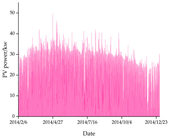
Figure 8.
Original PV power.
3.5. Validation of Combined Modal Decomposition
This paper adopts the method of combined decomposition to deeply explore the intrinsic connection between PV power and historical time series to decompose PV power. The average run time of the NARX-LSTM-LightGBM model is 45.23 min, and the average run time of the CD-NARX-LSTM-LightGBM model is 67.59 min.
For the three weather types, sunny, cloudy, and rainy days, the reference models, including LSTM, CD-LSTM, NARX-LSTM-LightGBM, and CD-NARX-LSTM-LightGBM, are constructed, respectively, for PV power prediction experiments contrast. Predictions were made for the above test days, and by observing Figure 9, it can be seen that the four models match the actual PV power prediction curves under sunny weather. The prediction models with combined modal decomposition in cloudy and rainy weather perform better, the prediction curves fit better with the real values, and the overall curves are consistent.
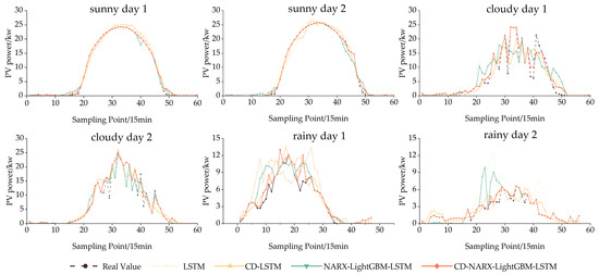
Figure 9.
The contrast of predicted and true values before and after modal decomposition.
Table 4 shows the results of the error–index contrast table, and Figure 10 shows the histogram stacking of prediction errors for the prediction of PV power by the four models (different colored areas indicate different prediction methods, and their smaller areas indicate smaller errors of the corresponding methods). For example, in the MAE in cloudy 1, the area of the rectangle representing CD-NARX-LSTM-LightGBM (red) is smaller than the area of the other models, and the area of the rectangle representing CD-LSTM (light blue) is smaller than the area of the rectangle representing LSTM (dark blue), and even smaller than the area of the rectangle representing NARX-LSTM-LightGBM (white). In RMSE, MAE, and MAPE, the CD-LSTM model reduces by 24.68%, 29.82%, and 29.82%, respectively, compared to the LSTM model, the CD-NARX-LSTM-LightGBM model compared to the NARX-LSTM-LightGBM model reduced by 56.30%, 58.45%, and 63.04%, respectively, and the CD-LSTM model reduces by 8.52%, 2.56%, and 13.04%, respectively, compared to the NARX-LSTM-LightGBM model. Overall, the prediction performance of the model is improved significantly by adding the high correlation sequence of the combined modal decomposition, and in some cases, the CD-individual model is even smaller than the combined prediction model error, which demonstrates that the machine learning model incorporated with the combined modal decomposition creates favorable conditions for improving the accuracy and reducing the uncertainty of PV power prediction.
Table 4.
The error of prediction results before and after combined modal decomposition.
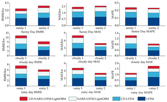
Figure 10.
Prediction error bar stacking chart.
3.6. Validation of the NARX-LSTM-LightGBM Model
This section further validates the performance of the CD-NARX-LSTM-LightGBM model for PV power prediction. For the three weather types, sunny, cloudy, and rainy days, combined decomposition reference models, including NARX, LSTM, LightGBM, RNN, and GRU, are constructed, respectively, for PV power prediction experiment contrast. The simulation results are shown in Figure 11.
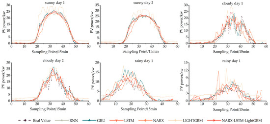
Figure 11.
CD-prediction model Contrast of predicted and real values.
According to Figure 11, It can be observed that the prediction performance depends greatly on the type of weather. Specifically, the prediction performance of the LightGBM model decreases significantly on cloudy and rainy days. The PV power has a large amplitude variation at certain times. This is due to characteristics such as high volatility and strong nonlinearity of environmental variables on cloudy and rainy days that directly impact the prediction results. With more detailed information comparing the original LSTM with the proposed model, it can be said that the predicted values and the error correction vector obtained from the initial NARX prediction and combinatorial machine learning models have significantly enhanced its performance in capturing the trend of the actual PV power. Overall, the proposed model performs the best, and its prediction performance of PV power is superior, especially in the two weather types of cloudy and rainy days, and its predicted power curve fits better with the real power curve.
Figure 12 shows the histogram stacking of prediction errors for the prediction of PV power by the six models, and Table 5, Table 6 and Table 7 show the contrast table of prediction errors. As can be seen from the figure, the area of the rectangle representing the error of the CD-NARX-LSTM-LightGBM model (red) is the smallest among the six models under any weather conditions. Specifically, according to the numerical results presented in Table 5, Table 6 and Table 7, LightGBM has poor prediction results compared to other models during sunny days, but it achieves good results during cloudy and rainy days. The mean RMSE for CD-NARX-LSTM-LightGBM is 1.654 kw and 0.884 kw for cloudy and rainy days, respectively, and the mean RMSE for rainy days is reduced by 46.55% compared to that for cloudy days. Take rainy days as an example, in which the mean RSME of CD-NARX-LSTM-LightGBM is 0.884 kw, while the closest model (CD-RNN) achieves a mean RMSE = 1.585 kw, and the proposed model has a 44.23% reduction in RMSE compared to CD-RNN. In summary, compared to individual models, the RMSE, MAE, and MAPE of CD-NARX-LSTM-LightGBM are lower than 1.665 kw, 0.892 kw, and 0.211, respectively for different weather types, which are better than the predictions of other models. The obtained results confirm the high performance of the proposed model in PV power prediction.
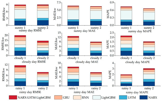
Figure 12.
CD-prediction model prediction error column stacking plot.
Table 5.
Different prediction model errors (sunny).
Table 6.
Different prediction model errors (cloudy).
Table 7.
Different prediction model errors (rainy).
4. Conclusions
The main objective of this study is to accurately predict PV power to achieve the integration of additional PV systems into the grid and to further improve energy management. This paper proposed a novel prediction framework based on the combination of NARX, LSTM, and LightGBM with the combination modal decomposition to predict PV power. The conclusions are as follows:
- The proposed model was effective at the accuracy of prediction as compared to an individual model, which has two apparent advantages. Firstly, the preliminary NARX prediction values and error correction vector features with high correlation coefficients (0.87 and 0.51, respectively) enhance the proposed model’s prediction performance in capturing the trend of the actual PV power. Furthermore, when large errors occur in individual models, the combination of prediction models by the inverse error method can largely reduce the impact on the accuracy of the prediction models;
- The original PV power was decomposed by EMD, EEMD, and CEEMDAN, and six groups of strong correlation sequences were obtained by correlation analysis, among which the highest correlation coefficient in EEMD was 0.925, which was second only to the irradiance correlation coefficient. The error of the model is obviously reduced after integrating the combined modal decomposition features. Taking rainy day 2 as an example, for RMSE, MAE, and MAPE, CD-LSTM is reduced by 55.12%, 39.88%, and 39.85%, respectively, compared to LSTM, and CD-NARX-LSTM-LightGBM is reduced by 57.19%, 25.43%, and 25.34%, respectively, compared to NARX-LSTM-LightGBM. It was demonstrated that the combined mode decomposition is strongly able to reduce the complexity of the original power curve and improve the accuracy of PV power prediction;
- The experiment results demonstrated that the proposed CD-NARX-LSTM-LightGBM achieved the lowest RMSE, MAE and MAPE, as compared to other models. The prediction stability of CD-NARX-LSTM-LightGBM is higher than other prediction methods, during the six test days the range of RMSE is stable in 0.399–1.664 kw, the range of MAE is stable in 0.136–0.892 kw, and the range of MAPE is stable in 0.015–0.221. The prediction effect of GRU fluctuates the most; the best RMSE can reach 0.897 kw, and the worst is only 3.690 kw;
- For all investigated PV systems, the proposed CD-NARX-LSTM-LightGBM model has invariably performed better than other models under different climatic conditions, indicating that the proposed model is superior and acceptable. The proposed model helps control the operation of the photovoltaic grid connection, making solar energy become a more economical, efficient, and reliable way to provide energy. Future work will expand the scope to include proposing models for other smart grid applications, including wind power and load prediction.
Author Contributions
Conceptualization, H.G. and J.W. (Jun Wang); methodology, H.G. and S.Q.; software, H.G. and J.F.; validation, H.G. and J.W. (Jun Wang); formal analysis, H.G. and N.M.; investigation, H.G., J.W. (Jiye Wang) and H.L.; resources, H.G. and K.C.; data curation, H.G. and D.H.; writing—original draft preparation, H.G.; writing—review and editing, H.G.; visualization, H.G. and S.Q.; supervision, H.G., J.F. and N.M. project administration, H.G., J.W. (Jiye Wang), K.C. and H.W.; funding acquisition, J.W. (Jun Wang), H.W. and Y.Z. All authors have read and agreed to the published version of the manuscript.
Funding
This research was supported by the Electric Power Research Institute of State Grid, Liaoning Electric Power Co., Ltd., and Technology Project (2022YF-83), and the Liaoning Province Scientific Research Funding Program (LJKZ0681).
Institutional Review Board Statement
Not applicable.
Informed Consent Statement
Not applicable.
Data Availability Statement
Not applicable.
Conflicts of Interest
The authors declare no conflict of interest.
Nomenclature
| PV | Photovoltaic |
| EMD | Empirical Mode Decomposition |
| EEMD | Ensemble Empirical Mode Decomposition |
| CEEMDAN | Complete Ensemble Empirical Mode Decomposition with Adaptive Noise |
| CD | Combined Decomposition (CD) |
| IMF | Intrinsic Mode Function |
| NARXNN | Nonlinear Auto-Regressive Neural Networks with Exogenous Input |
| LSTM | Long Short Term Memory |
| LightGBM | Light Gradient Boosting Machine |
| RF | Random Forest |
| SVM | Support Vector Machine |
| BP | Back Propagation |
| XGBoost | Extreme Gradient Boosting |
| RNN | Recurrent Neural Network |
| GRU | Gated Recurrent Unit |
| GOSS | Gradient-based One Side Sampling |
| EFB | Exclusive Feature Bundling |
| CD | Combined Decomposition |
| RMSE | Root Mean Square Error |
| MAE | Mean Absolute Error |
| MAPE | Mean Absolute Percentage Error |
References
- Singh, G.K. Solar power generation by PV (photovoltaic) technology: A review ScienceDirect. Energy 2013, 53, 1–13. [Google Scholar] [CrossRef]
- Zhou, J. Forecasting the Energy and Economic Benefits of Photovoltaic Technology in China’s Rural Areas. Sustainability 2021, 13, 8408. [Google Scholar]
- Kim, S.K.; Jeon, J.H.; Cho, C.H.; Kim, E.S.; Ahn, J.B. Modeling and simulation of a grid-connected PV generation system for electromagnetic transient analysis. Sol. Energy 2009, 83, 664–678. [Google Scholar] [CrossRef]
- Mahesh, K.; Perumal, N.; Irraivan, E. Optimal Placement and Sizing of Renewable Distributed Generations and Capacitor Banks into Radial Distribution Systems. Energies 2017, 10, 811. [Google Scholar]
- Liu, Z.; Sun, W.; Zeng, J. A new short-term load forecasting method of power system based on EEMD and SS-PSO. Neural Comput. Appl. 2014, 24, 973–983. [Google Scholar] [CrossRef]
- Mellit, A.; Pavan, A.M.; Lughi, V. Deep learning neural networks for short-term photovoltaic power forecasting. Renew. Energy 2021, 172, 276–288. [Google Scholar] [CrossRef]
- Almeida, M.P.; Perpinan, O.; Narvarte, L. PV power forecast using a nonparametric PV model. Sol. Energy 2015, 115, 354–368. [Google Scholar] [CrossRef]
- Holland, N.; Pang, X.; Herzberg, W.; Karalus, S.; Bor, J.; Lorenz, E. Solar and PV forecasting for large PV power plants using numerical weather models, satellite data and ground measurements. In Proceedings of the IEEE 46th Photovoltaic Specialists Conference (PVSC), Chicago, IL, USA, 16–21 June 2019; pp. 1609–1614. [Google Scholar]
- Kumar, M.; Soomro, A.M.; Uddin, W.; Kumar, L. Optimal Multi-Objective Placement and Sizing of Distributed Generation in Distribution System: A Comprehensive Review. Energies 2022, 15, 7850. [Google Scholar] [CrossRef]
- Belmahdi, B.; Louzazni, M.; El Bouardi, A. A hybrid ARIMA-ANN method to forecast daily global solar radiation in three different cities in Morocco. Eur. Phys. J. Plus 2020, 135, 1–23. [Google Scholar] [CrossRef]
- Bacher, P.; Madsen, H.; Nielsen, H.A. Online short-term solar power forecasting. Sol. Energy 2009, 83, 1772–1783. [Google Scholar] [CrossRef]
- Kim, S.-G.; Jung, J.-Y.; Sim, M.K. A Two-Step Approach to Solar Power Generation Prediction Based on Weather Data Using Machine Learning. Sustainability 2019, 11, 1501. [Google Scholar] [CrossRef]
- Fu, C.; Li, G.-Q.; Lin, K.-P.; Zhang, H.-J. Short-Term Wind Power Prediction Based on Improved Chicken Algorithm Optimization Support Vector Machine. Sustainability 2019, 11, 512. [Google Scholar] [CrossRef]
- Mo, H.; Zhang, Y.; Xian, Z.; Wang, H. Photovoltaic (PV) Power Prediction Based on ABC SVM. In Proceedings of the 1st International Conference on Environment Prevention and Pollution Control Technology (EPPCT), Tokyo, Japan, 9–11 November 2018. [Google Scholar]
- Balluff, S.; Bendfeld, J.; Krauter, S. Meteorological Data Forecast using RNN. Int. J. Grid High Perform. Comput. 2017, 9, 14. [Google Scholar] [CrossRef]
- Yj, A.; Jj, A.; Bk, B.; Suh, A. Long short-term memory recurrent neural network for modeling temporal patterns in long-term power forecasting for solar PV facilities: Case study of South Korea ScienceDirect. J. Clean. Prod. 2020, 250, 119476. [Google Scholar] [CrossRef]
- Gao, M.; Li, J.; Hong, F.; Long, D. Short-Term Forecasting of Power Production in a Large-Scale Photovoltaic Plant Based on LSTM. Appl. Sci. 2019, 9, 3192. [Google Scholar] [CrossRef]
- Gao, M.; Li, J.; Hong, F.; Long, D. Day-ahead power forecasting in a large-scale photovoltaic plant based on weather classification using LSTM. Energy 2019, 187, 115838. [Google Scholar] [CrossRef]
- Wang, K.; Qi, X.; Liu, H. Photovoltaic power forecasting based LSTM-Convolutional Network. Energy 2019, 189, 116225. [Google Scholar] [CrossRef]
- Yu, Y.; Cao, J.; Zhu, J. An LSTM Short-Term Solar Irradiance Forecasting under Complicated Weather Conditions. IEEE Access 2019, 7, 145651–145666. [Google Scholar] [CrossRef]
- Liu, R.; Asemota, G.N.O.; Benimana, S.; Nduwamungu, A.; Bimenyimana, S.; Niyonteze, J.D.D. Comparison of Nonlinear Autoregressive Neural Networks without and with External Inputs for PV Output Power Prediction. In Proceedings of the IEEE International Conference on Artificial Intelligence and Information Systems (ICAIIS), Dalian, China, 20–22 March 2020; pp. 145–149. [Google Scholar]
- Louzazni, M.; Mosalam, H.; Khouya, A.; Amechnoue, K. A non-linear auto-regressive exogenous method to forecast the photovoltaic power output. Sustain. Energy Technol. Assess. 2020, 38, 100670. [Google Scholar] [CrossRef]
- Yao, Q.; Song, D.; Chen, H.; Wei, C.; Cottrell, G.W. A Dual-Stage Attention-Based Recurrent Neural Network for Time Series Prediction. arXiv 2017, arXiv:1704.02971. [Google Scholar]
- Ming, C.; Jie, S.; Peide, L.; Qing, B. Comparative analysis of three machine learning algorithms in regression application. Intell. Comput. Appl. 2022, 12, 165–170. [Google Scholar]
- Wu, C.; Dong, A.; Li, Z.; Wang, F. Photovoltaic Power Prediction Based on Graph Similarity Day and PSO-XGBoost. High Volt. Eng. 2022, 48, 3250–3259. [Google Scholar]
- Chang, X.; Li, W.; Zomaya, A.Y. A Lightweight Short-Term Photovoltaic Power Prediction for Edge Computing. IEEE Trans. Green Commun. Netw. 2020, 4, 946–955. [Google Scholar] [CrossRef]
- Guo, Y.; Li, Y.; Xu, Y. Study on the application of LSTM-LightGBM Model in stock rise and fall prediction. In Proceedings of the 2nd International Conference on Computer Science Communication and Network Security (CSCNS), Sanya, China, 22–23 December 2020. [Google Scholar]
- Liang, Y.; Wu, J.; Wang, W.; Cao, Y.; Zhong, B.; Chen, Z.; Li, Z. Acm In Product Marketing Prediction based on XGboost and LightGBM Algorithm. In Proceedings of the 2nd International Conference on Artificial Intelligence and Pattern Recognition (AIPR), Beijing, China, 16–18 August 2019; pp. 150–153. [Google Scholar]
- Zhang, L.; Liu, M.; Qin, X.; Liu, G. Succinylation Site Prediction Based on Protein Sequences Using the IFS-LightGBM (BO) Model. Comput. Math. Methods Med. 2020, 2020, 8858489. [Google Scholar] [CrossRef]
- Wang, H.; Sun, J.; Wang, W. Photovoltaic Power Forecasting Based on EEMD and a Variable-Weight Combination Forecasting Model. Sustainability 2018, 10, 2627. [Google Scholar] [CrossRef]
- Haiwang, T.; Qiliang, Y.; Jiangchun, X.; Kefeng, H.; Shuo, Z.; Haoyu, H. Pgotovoltaic Power Prediction Based on Combined XGBoost-LSTM Model. Acta Energ. Sol. Sin. 2022, 43, 75–81. [Google Scholar]
- Zheng, Z.-W.; Chen, Y.-Y.; Zhou, X.-W.; Huo, M.-M.; Zhao, B.; Guo, M.-Y. Short-term prediction model for a Grid-Connected Photovoltaic System using EMD and GABPNN. In Proceedings of the International Conference on Sustainable Energy and Environmental Engineering (ICSEEE 2012), Guangzhou, China, 29–30 December 2012; p. 74. [Google Scholar]
- Yue, Z.; Jie, G.; Lu, M. Photovoltaic power generation prediction model based on EMD-LSTM. Electr. Power Eng. Technol. 2020, 39, 51–58. [Google Scholar]
- Zhongshan, L.; Jianhua, Y. Ultra-short term power prediction of photovoltaic power generation system based on EEMD-LSTM method. China Meas. Test 2022, 48, 125–132. [Google Scholar]
- Wang, S.; Liu, S.; Guan, X. Ultra-Short-Term Power Prediction of a Photovoltaic Power Station Based on the VMD-CEEMDAN-LSTM Model. Front. Energy Res. 2022, 10, 5327. [Google Scholar] [CrossRef]
- Zhang, N.; Ren, Q.; Liu, G.; Guo, L.; Li, J. Short-term PV Output Power Forecasting Based on CEEMDAN-AE-GRU. J. Electr. Eng. Technol. 2022, 17, 1183–1194. [Google Scholar] [CrossRef]
- Lilong, H.; Chao, Z.; Ping, Y. Research on Power Load Forecast Based on Ceemdan Optimization Algorithm. In Proceedings of the 3rd International Conference on Computer Information Science and Application Technology (CISAT), Electr Network, Dali, China, 17 July 2020. [Google Scholar]
- Kim, G.G.; Choi, J.H.; Park, S.Y.; Bhang, B.G.; Nam, W.J.; Cha, H.L.; Park, N.; Ahn, H.-K. Prediction Model for PV Performance with Correlation Analysis of Environmental Variables. IEEE J. Photovolt. 2019, 9, 832–841. [Google Scholar] [CrossRef]
- Zhong, J.; Liu, L.; Sun, Q.; Wang, X. Prediction of Photovoltaic Power Generation Based on General Regression and Back Propagation Neural Network. In Proceedings of the Applied Energy Symposium and Forum Low-Carbon Cities and Urban Energy Systems (CUE), Shanghai, China, 5–7 June 2018; pp. 1224–1229. [Google Scholar]
- Langley, B.P. Selection of relevant features and examples in machine learning. Artif. Intell. 1997, 97, 245–271. [Google Scholar] [CrossRef]
- Guihong, B.; Xin, Z.; Chenpeng, C.; Shilong, C.; Lu, L.; Xu, X.; Zhao, L. Ultra-short-term Prediction of Photovoltaic Power Generation Based on Multi-channel Input and PCNN-BiLSTM. Power Syst. Technol. 2022, 46, 3463–3476. [Google Scholar]
- Wang, S.; Zhang, N.; Wu, L.; Wang, Y. Wind speed forecasting based on the hybrid ensemble empirical mode decomposition and GA-BP neural network method. Renew. Energy 2016, 94, 629–636. [Google Scholar] [CrossRef]
- Colominas, M.A.; Schlotthauer, G.; Torres, M.E. Improved complete ensemble EMD: A suitable tool for biomedical signal processing. Biomed. Signal Process. Control 2014, 14, 19–29. [Google Scholar] [CrossRef]
- Lin, T.; Horne, B.G.; Tino, P.; Giles, C.L. Learning long-term dependencies in NARX recurrent neural networks. IEEE Trans. Neural Netw. 1996, 7, 1329–1338. [Google Scholar]
- Zina, B.; Octavian, C.; Ahmed, R.; Haritza, C.; Najiba, M.B. A Nonlinear Autoregressive Exogenous (NARX) Neural Network Model for the Prediction of the Daily Direct Solar Radiation. Energies 2018, 11, 620. [Google Scholar]
- Massaoudi, M.; Chihi, I.; Sidhom, L.; Trabelsi, M.; Refaat, S.S.; Abu-Rub, H.; Oueslati, F.S. An Effective Hybrid NARX-LSTM Model for Point and Interval PV Power Forecasting. IEEE Access 2021, 9, 36571–36588. [Google Scholar] [CrossRef]
- Abdel-Nasser, M.; Mahmoud, K. Accurate photovoltaic power forecasting models using deep LSTM-RNN. Neural Comput. Appl. 2017, 31, 2727–2740. [Google Scholar] [CrossRef]
- Zhou, H.; Zhang, Y.; Yang, L.; Liu, Q.; Du, Y. Short-term Photovoltaic Power Forecasting based on Long Short Term Memory Neural Network and Attention Mechanism. IEEE Access 2019, 7, 78063–78074. [Google Scholar] [CrossRef]
- Akhter, M.N.; Mekhilef, S.; Mokhlis, H.; Almohaimeed, Z.M.; Muhammad, M.A.; Khairuddin, A.S.M.; Akram, R.; Hussain, M.M. An Hour-Ahead PV Power Forecasting Method Based on an RNN-LSTM Model for Three Different PV Plants. Energies 2022, 15, 2243. [Google Scholar] [CrossRef]
- Hossain, M.S.; Mahmood, H. Short-Term Photovoltaic Power Forecasting Using an LSTM Neural Network. In Proceedings of the IEEE-Power-and-Energy-Society Innovative Smart Grid Technologies Conference (ISGT), Washington, DC, USA, 17–20 February 2020. [Google Scholar]
- Ke, G.; Meng, Q.; Finley, T.; Wang, T.; Chen, W.; Ma, W.; Ye, Q.; Liu, T.-Y. LightGBM: A Highly Efficient Gradient Boosting Decision Tree. In Proceedings of the 31st Annual Conference on Neural Information Processing Systems (NIPS), Long Beach, CA, USA, 4–9 December 2017. [Google Scholar]
- Bentejac, C.; Csorgo, A.; Martinez-Munoz, G. A comparative analysis of gradient boosting algorithms. Artif. Intell. Rev. 2021, 54, 1937–1967. [Google Scholar] [CrossRef]
- Anbo, M.; Xuancong, X.; Jiaming, C.; Chenen, W.; Tianmin, Z.; Hao, Y. Ultra Short Term Photovoltaic Power Prediction Based on Reinforcement Learning and Combined Deep Learning Model. Power Syst. Technol. 2021, 45, 4721–4728. [Google Scholar]
- Najibi, F.; Apostolopoulou, D.; Alonso, E. Enhanced performance Gaussian process regression for probabilistic short-term solar output forecast. Int. J. Electr. Power Energy Syst. 2021, 130, 106916. [Google Scholar] [CrossRef]
Disclaimer/Publisher’s Note: The statements, opinions and data contained in all publications are solely those of the individual author(s) and contributor(s) and not of MDPI and/or the editor(s). MDPI and/or the editor(s) disclaim responsibility for any injury to people or property resulting from any ideas, methods, instructions or products referred to in the content. |
© 2023 by the authors. Licensee MDPI, Basel, Switzerland. This article is an open access article distributed under the terms and conditions of the Creative Commons Attribution (CC BY) license (https://creativecommons.org/licenses/by/4.0/).