From Modeling to Optimizing Sustainable Public Transport: A New Methodological Approach

Abstract

This paper explores the potential for connected public-transport (PT) mobility as an alternative to motorized private transport (MPT) in medium-sized cities. Despite the high demand for MPT, it occupies a lot of space and contributes to conflicts and reduced livability. The more sustainable mobility solution of PT, however, is often considered slow, unreliable, and uncomfortable. To overcome these issues, the authors investigate the state-of-the-art research of connected PT mobility, including ways to quantify mobility behavior, micro- and macro-simulations of traffic flow, and the potential of not-yet-established modes of transport such as Mobility on Demand (MoD) for last-mile transportation. MoD could reduce the drawbacks of PT and provide sufficient and sustainable mobility to all citizens, including those in rural areas. To achieve this, precise information on individual traffic flows is needed, including origin–destination (OD) relations of all trips per day. The paper outlines a two-step approach involving the expansion of OD relations to include all modes of transport and diurnal variation, followed by microscopic traffic simulations and macroscopic optimization to determine potentials for on-demand offers within inner-city traffic. The paper concludes by calling for critical questioning of the approach to validate and verify its effectiveness.

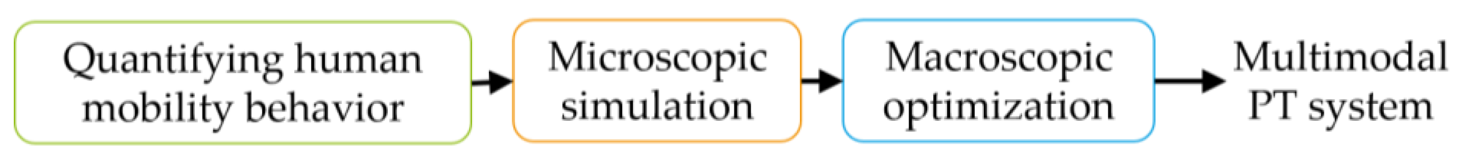
1. Introduction

Mobility nowadays is based on motorized private transport (MPT). Seventy-six percent of US commuters use their own vehicles to travel between home and work [1], whereas in Germany, 61% of commutes are executed by car. Even with a massive shift from internal-combustion-engine (ICE) cars to e-mobility, climate targets (e.g., [2]) will be difficult to reach if the current number of vehicles is maintained. Moreover, private cars burden the environment, as they occupy a lot of space. In the US, there is an average of eight parking spaces per car [3,4], and 5% of urban land is used by parking lots. This high demand for space results in conflicts between commuters and inhabitants of urban regions. Livability and health are often connected to the amount of motorized traffic [5]. Thus, for sustainable and livable cities it is important to reduce the number of cars and the amount of MPT mileage.

A more sustainable alternative to MPT commuting is using public transport (PT). Unfortunately, usage is hindered because PT is currently seen as expensive, overcrowded, unavailable, unreliable, and uncomfortable [6]. To address these issues and motivate commuters to use PT, innovative mobility solutions should be examined using state-of-the-art modeling and simulation methods. One example of an innovative solution is extending conventional, scheduled PT with new on-demand (OD) modes of transport.

Our contribution investigates the research of modeling multimodal mobility systems. We start by reviewing ways to quantify mobility behavior. If more than one mode of transport is used within one travelled distance, the trip is considered multimodal. The collected mobility data serve as a basis for micro- and macro-simulations of traffic flows. Based on these simulations, a valid evaluation of the potential of new (and not-yet-established) modes of transport becomes possible. One example of a new mode of transport is Mobility on Demand (MoD) for last-mile transportation. The vision of MoD is that rapid transit or bus connections with low station density and high travel speeds connect mobility hubs of rural areas. Regarding the adaptation of this innovative transportation mode, it has been shown that travelers’ attitudes regarding the sustainability of (possibly automated) OD vehicles is crucial [7]. MoD could thus solve the last-mile problem and connect mobility hubs with households, as well as provide short-distance door-to-door relations.

MoD could reduce the drawbacks of PT mentioned above and provide sustainable mobility even in rural areas, where inconvenient or slow point-to-point connections cause less acceptance of PT. MoD, understood as a ride-pooling service, could be used by ordinary PT fares as implemented in Hamburg [8]. From an economic perspective, this service can become a game changer, solving the current inconveniences of using PT if, at the same time, the expenses of MPT stay above the PT fare. In the largest German transport association, Rhine-Ruhr Transport Network, a passenger-kilometer of bus service results in a cost of EUR 30.69 [9]. With an average occupancy rate of 1.3 persons per car, the expenses per car-kilometer equal the PT costs per passenger of EUR 0.43. Compact cars from the fourth year onwards are likely to fall into this price category. Thus, PT is rarely more favorable than private cars, except in large metropolitan areas, where traffic volumes of 100,000 persons per day occur on many road sections.

These high traffic loads are rare in Germany. Despite an almost 77.5% urbanization rate [10], only 9.6% of the population lives in cities with more than one million inhabitants [11,12]. Thus, public transport is in the dilemma of either running too infrequently and being inconvenient or transporting too few customers at a time, resulting in more expensive tickets.

To provide a foundation for a more sustainable future of mobility, this paper examines how door-to-door mobility can be determined in medium-sized cities. Precise information on individual traffic flows is not publicly accessible for research, specifically the origin–destination (OD) relations of every trip per day. However, determining these OD relations in a time-resolved manner is the first step in investigating multimodal PT systems (see Figure 1). The output of this first step is an expansion of the OD relations to include all modes of transport and diurnal variation, which we refer to as the multimodal origin–destination–time matrix (MODTM or MODT matrix). The second step involves microscopic traffic simulations to estimate multimodal travel resistances, followed by macroscopic optimization to determine potentials for on-demand offers within inner-city traffic.

In the following sections, these steps will be explained using state-of-the-art methods. A critical review of the proposed approach should be performed to validate and verify the intent.

2. Quantifying Human-Mobility Behavior

The first step towards accessing the potential of mobility in medium-sized cities is to access the inhabitants’ current mobility data. Mobility data describes the movement of human beings in space and time, depending on the mode of transport used. These data can be used, for example, to improve traffic forecasts and urban or transport planning, (e.g., [13,14]), enhance our understanding of individual/group mobility [15,16,17], and increase the accuracy of predictions about future destinations [18,19]. Furthermore, mobility data have the potential to support various areas such as virus control [20,21], epidemic prevention [22], telecommunications [23], and energy and climate protection [24,25].

2.1. Accessing Mobility Behavior

Human-mobility behavior is characterized by trajectory patterns, modes of transport, locations of significance, and location-based activities [26]. These characterizations can be mapped in an MODTM. Interaction effects with other constructs have been highlighted in numerous previous studies. Examples include interactions with social-media-usage data on psychological stress [27], sleep data on well-being [28], and personality profiles on sustainable transportation [29].

In recent years, the number of mobility studies has increased significantly, as well as the diversity of topics, methods, and designs. Therefore, this section aims to provide an overview of existing designs and methods to quantify human-mobility behavior.

The period considered is one aspect in which mobility studies differ most in their design. It represents both how long data were collected per person or group and how long the entire survey took. In the past, conventional cross-sectional designs collected data on a single weekday within a certain period. However, since the late 1980s, continuous surveys considering longer periods and collecting data across one or several years have become increasingly popular [30,31]. Although some argue that long-term studies are essential to gaining a proper understanding of human-mobility behavior [32,33], both advantages and disadvantages are described in the literature. The advantages of continuous surveys are the possibility to control for seasonal effects, to capture specific and spontaneous events, to aggregate subsequent years, and to include flexible designs and additional questions. This is offset by higher costs, greater difficulties in data collection, higher dropout rates, and an increased risk of fatigue for both the participant and surveyor [31,33]. Therefore, the choice regarding the period for conducting future mobility studies should be made concerning the research question. At the same time, continuous surveys should not be seen as a one-size-fits-all solution, as it is sometimes misrepresented in the literature. Rather, appropriate observation periods should be used according to the research questions to achieve the best possible result.

2.2. Data-Collection Methods for Mobility Behavior

The choice of method for data collection has been shown to significantly impact the respondent’s broader engagement, making this the most important aspect in the design of human-mobility studies [34,35]. Regarding the survey methods used, a basic distinction should be made between systems based on personal interviews and those based on self-completion [31].

Personal interviews can further be distinguished between face-to-face interviews and telephone-based interviews. Face-to-face interviews have been used since the 1950s [36], mostly in the context of developing countries such as Chile or India [37,38]. The advantages of face-to-face interviews are the generally high response rates and the considerable flexibility, e.g., in collecting additional qualitative data [37], and the straightforwardness for participants [31]. Disadvantages of face-to-face interviews are the high costs [30,36] and (especially in comparison to self-completion forms) that the questionnaires must be answered at a certain time of day. Telephone-based interview methods, in comparison, have been implemented since the 1980s and 1990s [36] and are relatively cost-effective and therefore widely used, e.g., in North America [31]. Often, telephone interviews are conducted using an interactive computing system, leading the interviewer through the questions and allowing direct data entry [39]. This method is also known as computer-assisted telephone interviews (CATI). Telephone-based surveys were common in the past, to the extent that in the 1990s, non-telephone households would be excluded from mobility surveys [31]. Today, the disadvantage emerges that an increasing number of households are only reachable via a mobile phone number, which is rarely listed in publicly accessible databases.

Self-completion forms have thus gained importance in the collection of mobility data. Answers can be entered at a time suitable for the respondent, thus making the respondent burden easier [30]. It is advisable to focus on the design of the self-completion questionnaire and its ease of use, as this is the only direct contact with the participant [31]. Self-completion forms can be further distinguished by their format. Common formats are paper-and-pencil interviews (PAPI), as used in mail-out/mail-back surveys, computer-assisted web interviews (CAWI), and smartphone-based apps. In the first two mentioned formats, item-nonresponse errors are an issue, leading to fewer trips, as trips are incompletely reported or not reported at all [40].

PAPI, CAWI, and app-based surveys can be completed at any time and are normally completed by the respondents themselves. CAWI was introduced in mobility surveys in the early 21st century [36] to improve response rates by addressing population groups that are more inclined to use technology [41]. In comparison to paper questionnaires, online questionnaires offer advantages regarding the collection of responses (submitted with the questionnaire, do not have to be manually entered into a database), the accessibility of addresses (maps can be used to indicate locations directly), and implausibility prevention by logistics implemented in the questionnaire [42]. Moreover, based on earlier answers, only relevant questions can be shown to the participants, thus making the questionnaire easier to use [42]. Additionally, providing answers via common web browsers and smartphones can be helpful regarding accessibility, e.g., for people with impaired vision.

Within the last decade, mobility research has evolved with a new, automated way of accessing travel information using Global Navigation Satellite System (GNSS) measurements [43]. With the rise of smartphone use, apps have been used to retrieve mobility data and to generate travel diaries by combining various sensor data (e.g., location and acceleration) [36,42]. Apart from correction by the user, some of the apps offer the implementation of questionnaires that collect information about the respondent’s attitude towards certain aspects of mobility.

Apps provide one crucial advantage over PAPI, CATI, and CAWI: They are not dependent on the participant’s memory, which can help to prevent item-nonresponse and other accuracy errors [36]. Additionally, apps can be particularly useful for tracking multimodal trips, and the automated generation of travel diaries, combined with learning algorithms and suggestions, can further ease the respondent burden [35,44]. The disadvantages are technical issues and a lower response rate. There are reported problems with the accuracy of location data, which can vary across devices and with technical issues lying within the apps themselves and connected systematic, device-related dropouts [36]. Response rates are reported to be lower compared to CAWI, CAPI, and CATI [36,42], sometimes as low as 3%. A possible explanation is offered by the two key components of the technology-acceptance model—ease of use and usefulness—which were identified as influencing the intention to continue participating in the corresponding survey [45]. However, privacy concerns were not found to have a significant impact on dropout rates [45]. It can be assumed that dropout rates will continuously decrease as technology and usability improve. To address the aspect of usefulness, future studies on app-based mobility tracking should provide information and educate participants accordingly [36]. As mobility studies depend entirely on the motivation and conscientiousness of participants, regardless of the method used [35], it is essential to consider and address participants’ concerns and needs.

2.3. Using and Enhancing Mobility Data

In this section, we described and evaluated commonly used methods for quantification. We focused on methods based on the collection of actual mobility data of a certain period, thus accessing the OD data rather than relying on self-reported data from participants about their transportation habits and frequencies (e.g., [46]). Despite recent trends of using automatic generation of OD matrices via smartphone apps, a combination of more than one system is advisable. This contemplates the needs of different demographics and is also executed in the context of the German Mobility Panel [41].

Following the proposed path, current human-mobility behavior can be quantified with its trajectory patterns, modes of transport, and places of significance. This provides insight into the mobility of a specific group of participants. Further processing is required to extrapolate the OD data to the total population of the area of interest. Social and demographic attributes of the sample are queried and population groups with significant differences in mobility behavior are created. The mobility behavior of the sample is then extrapolated to the population groups’ actual size. To ensure the validity of the extrapolated mobility data, a validation process should be implemented. Existing traffic counts and other mobility data sets can be used for comparison and to determine whether the sample’s mobility is representative. Significant deviations need to be analyzed and may result in the calibration of the OD data.

3. Microscopic Traffic Simulation

In the second step, mobility behavior of the inhabitants of an example city and the resulting traffic flow are simulated. A suitable microscopic traffic-flow model is necessary to be able to make predictions about the result of adjustments to the macroscopic traffic situation and the selected road-network section. This means, for example, a change in frequency of public transport, the addition of other modes of transport, or limitations to private transport.

There are several tools for traffic-flow simulation, including Multi-Agent Transport Simulation (MATsim) [47] and open-sources tools like “Simulation of Urban Mobility” (SUMO), which follows a different modeling approach and is not focused on PT. SUMO offers many advantages over commercial simulation software like PTV Vissim [48], TransModeler [49], and Aimsum [50]. SUMO supports many data formats, simplifying the process of importing data from other sources, such as GPS data and road-network information of open-source map providers. In addition, SUMO has a strong focus on public-transport simulation, which is suitable for projects related to PT. It has the largest user community and many online resources, which provide an easy start for new users while being highly adaptable and customizable. Although both commercial simulation software and SUMO have their advantages, SUMO is a better choice for many applications due to its lower cost, wide range of in- and output formats, and strong focus on PT simulation. It is well suited for both academic and commercial projects, making it a versatile tool for traffic simulation.

Therefore, SUMO from the German Aerospace Center is the tool of choice for the simulation of a microscopic traffic-flow simulation [51]. This tool offers the possibility to use a selected map section of an open-source map provider such as OpenStreetMap [52] to generate node (junctions) and edge (roads) networks in a fast, resource-efficient, and customizable way. In the simplest case, a randomized traffic flow can be applied to the road network. Common modes of transport can be included in the consideration, provided that the corresponding effort is put into the adaptation of the automatically generated nodes and edges. Figure 2 shows the above-mentioned city provided by OpenStreetMap in the upper half. In the lower half, the road network converted by Netedit is shown. Netedit is a graphical network editor included in SUMO. This has already been assigned a randomized traffic flow, which can be seen within the magnifying-glass visualization.

To minimize the post-processing effort, the first goal is to improve the automatic generation and parameterization of nodes and edges, as well as their dependencies. This is particularly crucial because the aim is not solely to represent a single specific city or region. Rather, the transferability to any area should be ensured. Since the modeling of a whole city or a large region is quite complex or even impossible for a non-expert, e.g., the corresponding PT association, an easy-to-use tool must be developed. This task should be specified in the discussion (see Section 5).

A validation of the simulation should first be completed for the exemplarily chosen city by extending the generated MODTM with a mathematical model based on existing research results [53,54,55,56]. This model includes determined travel resistances for different modes of transport, which will allow us to draw conclusions about both mode choice and occupancy levels.

In the context of SUMO, it must be possible to use and process a known MODTM. Currently, OD matrices with defined start and end edges or traffic-assignment zones (TAZ) can be used within the framework. These zones serve to describe the traffic flow between districts over time. However, we still need to incorporate the surveyed and extrapolated mode of transport into the simulation to reflect the complete information content of an MODTM. One way to do this is to divide the complete MODTM by transport modes and create an OD matrix for each mode that describes the surveyed mobility behavior between districts (or TAZs) over discrete time periods. As soon as this procedure is complete, we can start to further implement and investigate topics such as MoD. This brings us to the well-known problem of time-dependent vehicle-routing problems.

To simulate MoD, especially the benefits at off-peak hours, the vehicle-routing problem needs to be time dependent and take flexible departure times of passengers into account. Ref. [57] completed some pioneering work in formulating time-dependent vehicle-routing problems (TDVRP) with certain heuristics. Refs. [58,59] adapted the well-known methods of branch and price and branch and cut to solve TDVRP. Ref. [60] formulated TDVRPs with soft and hard time windows to take flexible travel demands into account. Ref. [61] solved TDVRPs with soft time windows and stochastic travel times due to traffic congestion by using a tabu search and an adaptive large-neighborhood search. Ref. [62] use a tabu search and the ant-colony system in a supply chain and recycling TDVRP. Those examples and most other approaches found in the literature used heuristics to solve TDVRPs [63] and therefore applied to a few specific use cases only. Which method fits best as a basis for our approach remains to be analyzed in further research.

Thus, from a microscopic point of view, SUMO can be used to simulate when and how travelers move between places in different transport modes. In Section 4, we will look at the resulting travel resistance and the extent to which a targeted use of MoD can improve the traffic flow in the region under consideration.

4. Macroscopic Multimodal Public-Transport Model

The third and final step of the suggested approach (see Figure 1) describes the macroscopic multimodal PT model, which is necessary to optimize the given parameters (e.g., the size of the MoD fleet, travel resistances, etc.).

In the second half of the 20th century, PT systems were mathematically modeled by various means. The vast majority utilized mathematical-network problems to describe the spatiotemporal mobility behavior and vehicle routes. A fundamental mathematical-programming model of a general PT network and an optimization procedure to schedule bus-departure times were developed in 1976 [64] under known deterministic conditions. Further development in computer-science and operations research enabled more degrees of freedom and more complex network-flow problems [65]. Some famous examples are vehicle-routing problems (see Section 3) and shortest-path problems, which are relevant to the MoD model. The time-dependent expansion of network problems is especially relevant for this contribution to model the supplement of MoD in PT at off-peak times.

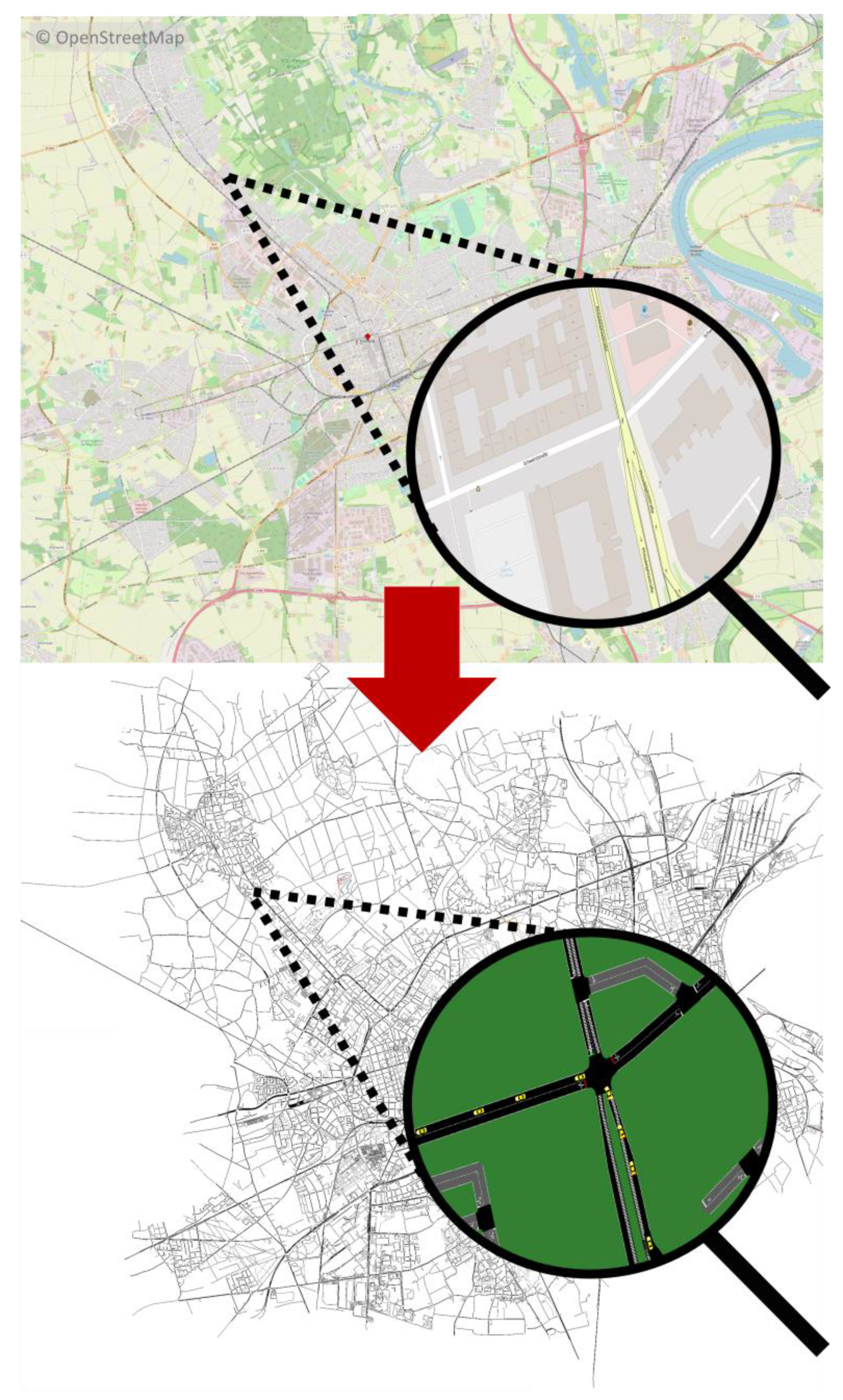
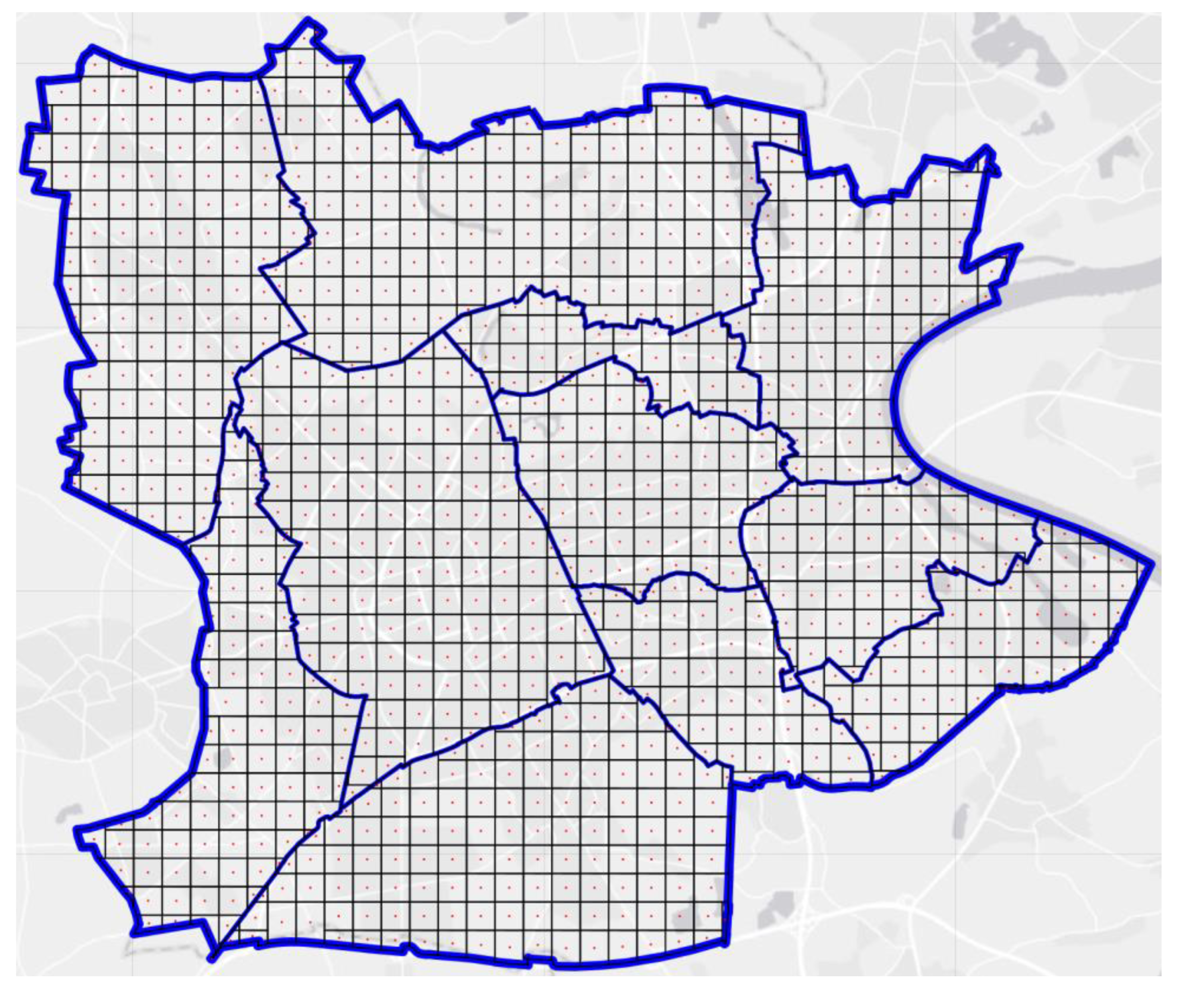
4.1. Discretization of the Area under Investigation

For traffic analyses on a macroscopic level, the size of traffic cells (see TAZ, Section 3) usually represents the districts of the investigated city [66]. This leads to bulky zone sizes of a few square kilometers, which are too inaccurate to model local transport, especially the last-mile problem. The average path of PT users from their residence to their next destination is approx. 5 min or 375 m [66]. Traffic cells in studies including local PT should be sized in this scale to minimize inaccuracy due to discretization (see Figure 3). Footpaths to or from a stop or station need to be considered, because they are a common reason for not using PT.

Macroscopic means that the spatiotemporal resolution is still high, but other than in microscopic simulations (see Section 3), persons or vehicles are not considered. The model aggregates the number of travelers for each cell and time step to save computational time and to solve linear-programming problems in polynomial time.

Our approach is based on the previous project MobilitätsWerkStadt 2025, in which a 400 × 400 m grid of traffic cells led to negligible small deviations in approaching PT [54]. In this example, the grid contained 866 cells with 749,090 possible OD relations. Every mobility demand could be assigned to one of these relations.

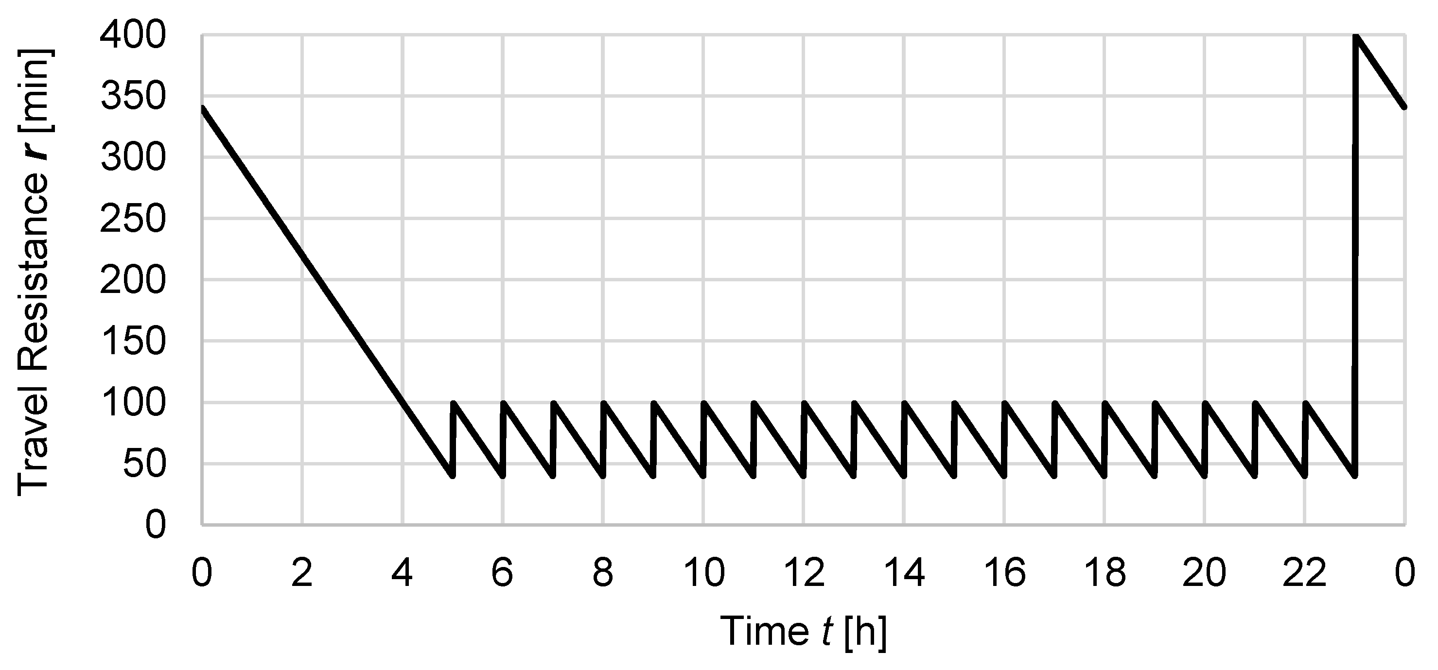
4.2. Public-Transport Travel Resistances

The German Ministry of Transport commissioned the development of a method for rail-bound PT investments [67]. Different modes of transport are made comparable by modeling inconveniences (e.g., waiting times, searching for parking space, changing into other PT lines, or walking distances to stations) with travel-time equivalents. The sum of the actual travel time and the equivalent on a relation is defined as the travel resistance r specified in minutes. For PT, each relation from origin i to destination j has a different value of r, summarized in a matrix R, which is defined as follows [67]:

$$\begin{gathered} R_{ij,\mathrm{P}\mathrm{T}}=R_{approach}+R_{stationEntry}+{\sum }_{PP}\left(R_{inVehicle,PP}\right)+{\sum }_C\left(R_{footwayChange}+ \\ {R}_{wait,PP}+R_{change}+R_{stationChange}\right)+R_{departure}+R_{stationExit} \end{gathered}$$

(1)

with

• $R_{ij,\mathrm{P}\mathrm{T}}$: travel resistance of relation from origin i to destination j with PT;
• $R_{approach/departure}$: travel resistance of approaching or departing PT;
• $R_{stationEntry/Change/Exit}$: additional resistance of station due to insufficient amenities;
• $R_{inVehicle,PP}$: rated travel time of part of the path;
• $PP$: part (section) of the whole path;
• $R_{footwayChange}$: rated travel time of the footpath between stations;
• $R_{wait,PP}$: travel-time equivalent for waiting times while changing mode of transport;
• $R_{change}$: travel-time equivalent for additional inconveniences of changing mode of transport (except waiting times).

For example, the travel-time equivalent $R_{approach}$, representing a footpath to a station with a certain length $t_{approach}$ specified in minutes, can be calculated by:

$$R_{approach}=t_{approach}\times \left(0.9+0.15\times t_{approach}\right),$$

(2)

with

• $t_{approach}$: time to approach PT in minutes.

This method needs to be comprehensive and applicable and therefore uses some simplifications to be computable. The total number of bus trips per day on a certain relation, the cycle time, and many other factors as input variables lead to a simple scalar output variable r for public and private transport.

The temporal distribution of the number of bus trips between two bus stops can affect service quality. For example, if two bus lines connect at the same two stops, the following deviation occurs. The first bus departs at 6 a.m., 7 a.m., …, 9 p.m. If the second bus departed at 6:01 a.m., 7:01 a.m., …, 9:01 p.m., the total service quality between the two bus stops would be significantly worse compared to another case with the second bus departing at 6:30 a.m., 7:30 a.m., …, 9:30 p.m. The method mentioned above [67] does not consider this, simplifying the issue by using the total number of bus trips per day, which would be the same in both cases.

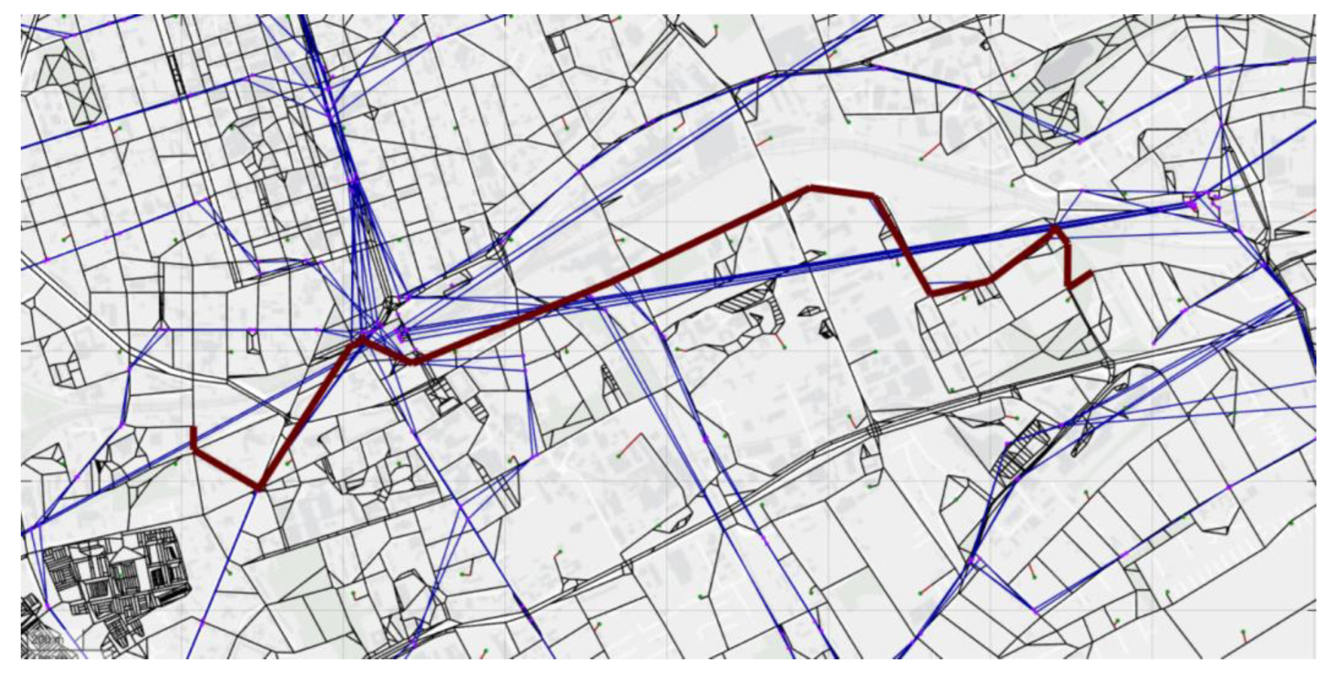
4.3. Time-Dependent-Directed Graph

For decades, public-transit systems such as buses and trams have been modeled using directed and weighted graphs. Nodes represent stations and can include information such as location, name, wheelchair accessibility, seating, and nearby shops. Edges represent connections between two stations with any PT mode and can include information such as capacity limits, operating company, assigned route name or line number, or Wi-Fi availability. The weight of an edge is usually given by travel time, so shortest-path algorithms find the fastest path between start and destination nodes. In time-dependent graphs, the weight of an edge is a vector or time-dependent function that considers departure times and models different travel times in a daily variation due to traffic jams or varying cycle times.

4.4. Time-Dependent Shortest-Path Algorithm with Multidimensional Edge Weights

Shortest-path problems find the fastest path between start and destination nodes (see Figure 4), with edges weights typically representing costs that need to be minimized [68,69,70,71]. Distances as edge weights result in the shortest path; travel time as edge weights result in the fastest path.

In this approach, the objective is to minimize the travel resistances r of a PT system, meaning that the best path between two nodes equals the one with the minimum r, which might differ to the path with minimum travel time $\mathit{t}$. Therefore, the edge weight is set to r. If r is a time-dependent sawmill function (see Section 5), the shortest-path algorithm also needs to know when the person arrives at a node. That means that t is added as a second edge weight to compute the arrival time at each node in the graph. Both $\mathit{t}$ and $\mathit{r}$ are time-dependent functions. If the timestep is set to one minute and the observation period is set to one day, the edge weight corresponds to $\mathit{W}\in {\mathbb{R}}^{2\times 1440}$.

Alternative approaches, which already have implemented multidimensional edge weights with sawmill time-dependent travel times, were not found in the common literature. Such an algorithm will be implemented in further research by the authors. One promising approach could be to adapt and extend well-known optimization methods such as the A*-Algorithm [71].

4.5. Constant Travel Resistances of Transfers in Graph Theory

To model the inconvenience of changing public transport, a constant travel-time equivalent of eight minutes is added to the waiting time and walking distance to the next station [67]. Waiting times are considered by the function of the departure times of an edge, whereas walking distances between stations can be modeled by separate edges. To model the constant equivalent of eight minutes, a control variable is added to the implementation of the shortest-path algorithm and concatenates the different lines used. For each different PT line used in the path from the origin node to the destination node, the constant travel-time equivalent is added to the total travel resistance.

4.6. Travel Resistances of Motorized Private Transport, Cycling, and Footpaths

Computing travel resistances for MPT, cycling, or by foot between an origin and destination node can be achieved by publicly available data [54,56]. This approach uses floating car data to find the actual travel times on streets, including congestion and traffic-light settings for different times of day. Evaluating parking-space availability is difficult and, to this day, has not been solved by using publicly available data. Other studies use a different approach by assuming the average search time for parking spaces [72,73,74]. Some cities have parking-space management systems and can deduce the real-time available parking space in a whole district with sensors installed in some parking lots. It is challenging to obtain parking-space availability by calculating the number of vehicles in a district and comparing it to the number of available parking spaces, because maps of parking spaces do not contain the number of parking lots at the roadside, which can also vary due to different vehicle sizes and parking behavior.

4.7. Macroscopic Modeling of Mobility on Demand

To insert MoD systems into the macroscopic graph structure for the optimization (see Section 4.9), average waiting and driving times between all traffic cells based on the size of the vehicle fleet, size of the service area, and operating hours must be depicted by microscopic traffic simulations (see Section 3) and using validated and up-to-date OD matrices as described (see Section 2).

4.8. Economic Point of View

To find the optimal PT system with certain boundary conditions, the objective function must consider economic indicators. Initial and operating costs are modeled using simplified key performance indicators (see

Table 1. Operating costs of a PT vehicle (cf. [75]).

Per Operating Hour	Per Year	Per Kilometer
Driver’s wage	Insurance	Energy
Employee training	Inspection	Tires
Monitoring	Overhead	Maintenance
Additional services

).

4.9. Optimization Problem

The above-described macroscopic model can allocate travel demand from OD data (see Section 2) to the mode of transport by comparing travel resistances. In other words, it computes the modal split of a certain transport offer. The number of people buying a monthly ticket subscription and the number of individual tickets in PT can be estimated, which results in the revenue of PT companies. Additionally, the model computes the costs to provide this mobility offer.

The optimizer can change the mobility offer by allocating the vehicles to other spatiotemporal routes and by adding vehicles or routes. Several boundary conditions must be considered, such as school transport, the municipal PT plan, and the mobility guarantee provided by a local-transport operator.

There can be several (multi-)objective functions set up with the aforementioned method, combined with educated assumptions and additional constraints:

• Minimize average public-transport travel resistance of all relations or maximize the modal shift with today’s investments as the maximum budget.
• Minimize cost or maximize revenue with today’s travel resistances.
• Minimize government subsidies to get a modal split of 30%, 40%, …, or 60% PT.
• Minimize CO₂ emissions with a certain amount of government subsidies.

In summary, the third step benefits from renowned methods from graph theory and operations research and combines them with proven methods of feasibility studies, enabling an innovative approach to improve the planning of extending PT systems with MoD or other new modes of transport. However, the described inaccuracies of travel resistances need to be addressed in further research, which is elaborated in Section 5.

5. Summary of Results

This contribution aims to outline an approach to determine the effect of future door-to-door mobility on the modal shift from MPT to PT. The presented methods can be used or adapted by municipal-traffic planners and research institutes to conduct a cost–benefit analysis in their local context. To our knowledge, there are no publicly available studies considering economic and environmental efficiency or the attractiveness of regular transport services extended with MoD. Our contribution identifies the complexity of today’s issues of modeling multimodal transport systems to their full extent.

Based on state-of-the-art research, we derived three steps, shown in Figure 5. Quantifying human-mobility behavior is complex but crucial for any further analysis. Compared to other state-of-the-art methods presented in Section 2, we propose using a highly resolved MODTM and an analysis of the choice of mode of transport based on quality. The quality of a mode of transport can be modeled with travel resistances, as shown in Section 4.2. This enables the prediction of modal shifts in step three (see left arrow in Figure 5). To compute the travel resistances of MoD systems, their average occupation rates, travel speeds, and waiting times (KPIs of MoD) must be determined by microscopic traffic simulations. The latest challenges using SUMO, the furthest developed open-source software—easily accessible for every municipal traffic planner—are explained in Section 3. The input parameter of the microscopic simulation could be the size of the additional vehicle fleet. The resulting KPIs of MoD are used to compute the travel resistance for every edge of the macroscopic graph. Section 4.4 explains the characteristics of time-dependent graphs and shortest-path algorithms. Along with the mathematical functions to describe the choice of mode of transport, the macroscopic traffic model can compute the modal split for every OD relation. During the optimization, edges representing MoD trips can be added or removed from the graph. Every added edge increases the investment and operating costs of the public-transport system. With any of the objective functions described in Section 4.9, the optimal size of the traffic fleet can be computed.

This approach secures investment in MoD fleets and helps municipal-traffic planners to establish the most efficient public-transport system from an environmental and economic point of view.

6. Discussion

Today, the necessary computing power exists to implement the modeling approach presented in this study, which aims to simulate the potential impacts of tomorrow’s mobility on current transportation systems. Section 2 summarizes and evaluates various survey methods and designs to access current mobility behavior. We recommend a combination of methods to collect a broad number of data and further validation with publicly available data. The resulting matrix contains validated information on inhabitants’ door-to-door mobility behavior and constitutes the foundation of the following two steps. Our approach is based on minimizing travel resistance and optimizing travel time. In addition, mobility behavior and especially its adaptation to new developments are also influenced by psychological aspects, which are not considered in our simulation.

The second step shows a way of integrating the resulting MODT matrix in the traffic-flow simulation by using the SUMO tool. The manual reworking of intersections and traffic lights in SUMO can be particularly challenging for increasing city sizes or regions due to the number and complexity of intersections and traffic-light logistics. This can be time-consuming, making the simulation process impractical. In addition, the process can be even more time-consuming for untrained users of SUMO, as they may not be familiar with the tools and techniques or know what to do to realistically implement various intersection situations. For this reason, software must be created that guides the user through the creation and evaluation of the traffic-flow scenario step by step. Not only should the map data of the selected city or region be included but all relevant data should also be available to the user. The resulting tool should be able to use and interpret different data sets to improve the accuracy of the model. For example, it should be possible to include existing PT schedules and public standardized schemes for switching traffic signals. Special attention should be given to the possibility of using and integrating collected MODTM to create a demand-responsive traffic scenario (see Section 2).

The third step includes generating a macroscopic traffic model representing all modes of transport with the help of graph structures and travel resistances as edge weights. Section 4 presents current standards in graph theory and a critical analysis of travel resistances. This model can compare different modes of transport for every single spatiotemporal mobility demand and predict modal shifts due to changes in mobility offers. By optimizing graphs, nodes, and edges using well-known methods, we can modify, enlarge, or leave out elements to find the optimum public-transport system under certain constraints. An objective function could be maximizing the modal shift from MPT to PT, whereas a possible constraint could be cost neutrality. The input parameter of the optimization could be the size of the MoD car fleet. To ensure realistic results of the macroscopic optimization, the final parameters can be checked in a feedback loop with the microscopic simulation of step 2.

To overcome the described inaccuracies of travel-resistance calculations, some modifications must be made. A detailed temporal resolution of travel resistances needs to be considered to optimize MoD services and their benefits at off-peak hours.

Calculating the travel resistance for every time step of an investigated period leads to a sawtooth function (see Figure 6). In this simplified case, travel resistance r is calculated minute-wise, corresponding to $\mathit{r}\in {\mathbb{R}}^{1440}$, for a bus connection that departs hourly from 5:00 a.m. to 11:00 p.m. The minimum values of r represent the sum of the walkways to/from the station and the driving time. The person boards the bus just in time. Every other higher value includes additional waiting times. The peaks of the sawtooth function represent the case of just missing a bus and waiting for the next to come. The function could be used as an edge weight of the public-transport graph.

Our optimization framework can address various issues, such as analyzing scenarios that compare the initial costs of highly automated vehicles with the operating costs. The simulated scenarios can investigate (upcoming) behavioral intentions. This leads the way to estimating possible utilization rates and thus exploring under which economic conditions highly automated OD vehicles are commercially self-supporting. In addition, psychological factors influencing mobility behavior, e.g., sustainability attitudes, can be investigated [76,77].

Predictions regarding the MPT development show a significant increase of around 10% until 2030 [78], which further stresses the need for more sustainable modes of transport. This is especially relevant since the transport sector in Germany missed the sector target of the Climate Protection Law significantly by more than 9 million t CO₂ eq. in 2022 [79]. Our approach can contribute to the mobility transition by taking different carbon-pricing schemes into account and rating their effects on the modal shift.

Focusing on public transportation, we consider the potential impact that better infrastructure can have on mobility-impaired people and low-income households [80]. Our approach provides a reliable foundation for investment decisions in municipal transportation companies, which in Germany are often financed by public means and must bear public and social responsibility, e.g., by making their mobility offer accessible.

Compared to commercial software, our approach aims to provide an open-source base that is easily accessible and uses hands-on methods to process a variety of data sets. This enables a community-driven optimization tool benefiting from interdisciplinary developers and users.

The outlined approach could be limited by focusing on the simulation of mobility within a medium-sized city, leaving out transregional traffic, e.g., from adjoining cities. Another limitation emerges in the database of our simulation: It rests on accessed and enriched mobility behavior. Following the mobility-biography approach, this behavior is subject to continuous change, e.g., because of major life events [81]. Extending public-transport offers can affect traffic demands. Autonomous vehicles in particular might favor urban sprawl [82]. Therefore, it is crucial to use current mobility data and renew these data on a regular basis—in particular, after introducing a possible new mode of transport.

Despite these limitations, our contribution sets the ground for the evaluation of future mobility modes. Therefore, an interdisciplinary approach to modeling multimodal public-transport systems should be implemented, as it leads the way to a more knowledge- and simulation-based evolution of modes of transport. This research introduces a novel approach for modeling multimodal transport systems in medium-sized cities. It integrates microscopic traffic simulations and macroscopic public-transport models to evaluate mobility behavior and modal shifts. The study incorporates economic indicators to assess the economic viability of different transport modes and emphasizes sustainability, social responsibility, and the importance of open-source collaboration in transportation planning. Overall, we offer a comprehensive framework that considers various factors in optimizing transport systems and supports the transition towards sustainable and efficient mobility.

7. Conclusions

Our contribution outlines a transferable approach to model mobility behavior within highly populated regions and enhances existing public infrastructure, e.g., with MoD services. The simulation builds the foundation for the implementation of any future mode of transport even under economic-boundary conditions. The presented approach therefore is not only of theoretical value but also highly relevant for a sustainable mobility transition.

References

- United States Department of Transportation. Transportation Statistics Annual Report 2021; United States Department of Transportation: Washington, DC, USA, 2020.
- United Nations. The Paris Agreement: United Nations Framework Convention on Climate Change; United Nations: New York, NY, USA, 2015.
- Crawford, J.H.; Verner, A. Carfree Cities; International Books: Dublin, Ireland, 2000. [Google Scholar]
- Eckersley, R.; Dixon, J.; Douglas, R.M.; Douglas, B. The Social Origins of Health and Well-Being; Cambridge University Press: Cambridge, UK, 2001. [Google Scholar]
- Oviedo, D.; Sabogal, O.; Villamizar Duarte, N.; Chong, A.Z.W. Perceived liveability, transport, and mental health: A story of overlying inequalities. J. Transp. Health 2022, 27, 101513. [Google Scholar] [CrossRef]
- Statista. Wieso nutzen Sie die öffentlichen Nahverkehrsmittel nicht öfter? Statista: Hamburg, Germany, 2019. [Google Scholar]
- Yap, M.D.; Correia, G.; van Arem, B. Preferences of travellers for using automated vehicles as last mile public transport of multimodal train trips. Transp. Res. Part A Policy Pract. 2016, 94, 1–16. [Google Scholar] [CrossRef]
- Verkehrsbetriebe Hamburg-Holstein GmbH. Ein On-Demand-Angebot als Teil des hvv. Available online: https://vhhbus.de/hop/ (accessed on 28 March 2023).
- AöR, V.R.-R. Ausbildungsverkehr-Richtlinie AusbV-RL. 2019. Available online: https://zvis.vrr.de/bi/vo0050.asp?__kvonr=6064 (accessed on 23 March 2023).
- Bank, W. Urbanisierungsgrad: Anteil der Stadtbewohner an der Gesamtbevölkerung in Deutschland in den Kahren von 2000 bis 2021; Statista: Hamburg, Germany, 2022. [Google Scholar]
- Bundesamt, S. Bevölkerungsstand: Amtliche Einwohnerzahl Deutschlands 2022. Available online: https://www.destatis.de/DE/Themen/Gesellschaft-Umwelt/Bevoelkerung/Bevoelkerungsstand/_inhalt.html (accessed on 23 March 2023).
- Statista. Einwohnerzahl der größten Städte in Deutschland am 31 Dezember 2021. Available online: https://de.statista.com/statistik/daten/studie/1353/umfrage/einwohnerzahlen-der-grossstaedte-deutschlands/ (accessed on 23 March 2023).
- Makse, H.A.; Havlin, S.; Stanley, H.E. Modelling urban growth patterns. Nature 1995, 377, 608–612. [Google Scholar] [CrossRef]
- Xu, F.; Li, Y.; Jin, D.; Lu, J.; Song, C. Emergence of urban growth patterns from human mobility behavior. Nat. Comput. Sci. 2021, 1, 791–800. [Google Scholar] [CrossRef]
- Benita, F. Human mobility behavior in COVID-19: A systematic literature review and bibliometric analysis. Sustain. Cities Soc. 2021, 70, 102916. [Google Scholar] [CrossRef] [PubMed]
- Han, S.Y.; Tsou, M.-H.; Knaap, E.; Rey, S.; Cao, G. How do cities flow in an emergency? Tracing human mobility patterns during a natural disaster with big data and geospatial data science. Urban Sci. 2019, 3, 51. [Google Scholar] [CrossRef]
- Gonzalez, M.C.; Hidalgo, C.A.; Barabasi, A.-L. Understanding individual human mobility patterns. Nature 2008, 453, 779–782. [Google Scholar] [CrossRef]
- Do, T.M.T.; Gatica-Perez, D. Contextual conditional models for smartphone-based human mobility prediction. In Proceedings of the 2012 ACM Conference on Ubiquitous Computing, Pittsburgh, PA, USA, 5–8 September 2012; pp. 163–172. [Google Scholar]
- Song, C.; Koren, T.; Wang, P.; Barabási, A.-L. Modelling the scaling properties of human mobility. Nat. Phys. 2010, 6, 818–823. [Google Scholar] [CrossRef]
- Vazquez-Prokopec, G.M.; Bisanzio, D.; Stoddard, S.T.; Paz-Soldan, V.; Morrison, A.C.; Elder, J.P.; Ramirez-Paredes, J.; Halsey, E.S.; Kochel, T.J.; Scott, T.W. Using GPS technology to quantify human mobility, dynamic contacts and infectious disease dynamics in a resource-poor urban environment. PLoS ONE 2013, 8, e58802. [Google Scholar] [CrossRef]
- Hadjidemetriou, G.M.; Sasidharan, M.; Kouyialis, G.; Parlikad, A.K. The impact of government measures and human mobility trend on COVID-19 related deaths in the UK. Transp. Res. Interdiscip. Perspect. 2020, 6, 100167. [Google Scholar] [CrossRef]
- Du, B.; Zhao, Z.; Zhao, J.; Yu, L.; Sun, L.; Lv, W. Modelling the epidemic dynamics of COVID-19 with consideration of human mobility. Int. J. Data Sci. Anal. 2021, 12, 369–382. [Google Scholar] [CrossRef]
- Andrade, T.; Cancela, B.; Gama, J. Discovering locations and habits from human mobility data. Ann. Telecommun. 2020, 75, 505–521. [Google Scholar] [CrossRef]
- Archer, C.L.; Cervone, G.; Golbazi, M.; Al Fahel, N.; Hultquist, C. Changes in air quality and human mobility in the USA during the COVID-19 pandemic. Bull. Atmos. Sci. Technol. 2020, 1, 491–514. [Google Scholar] [CrossRef]
- Schaefer, A.; Jacoby, H.D.; Heywood, J.B.; Waitz, I.A. The Other Climate Threat: Transportation: A global travel surge is inevitable, but runaway growth of mobility-related CO2 emissions is not. Am. Sci. 2009, 97, 476–483. [Google Scholar] [CrossRef]
- Lin, M.; Hsu, W.-J. Mining GPS data for mobility patterns: A survey. Pervasive Mob. Comput. 2014, 12, 1–16. [Google Scholar] [CrossRef]
- Jin, L.; Xue, Y.; Li, Q.; Feng, L. Integrating human mobility and social media for adolescent psychological stress detection. In Proceedings of the International Conference on Database Systems for Advanced Applications, Dallas, TX, USA, 16–19 April 2016; pp. 367–382. [Google Scholar]
- DeMasi, O.; Feygin, S.; Dembo, A.; Aguilera, A.; Recht, B. Well-being tracking via smartphone-measured activity and sleep: Cohort study. JMIR Mhealth Uhealth 2017, 5, e7820. [Google Scholar] [CrossRef]
- Anagnostopoulou, E.; Urbančič, J.; Bothos, E.; Magoutas, B.; Bradesko, L.; Schrammel, J.; Mentzas, G. From mobility patterns to behavioural change: Leveraging travel behaviour and personality profiles to nudge for sustainable transportation. J. Intell. Inf. Syst. 2020, 54, 157–178. [Google Scholar] [CrossRef]
- Ampt, E.S.; de Dios Ortúzar, J.; Richardson, A.J. Large-scale ongoing mobility surveys: The state of practice. In Transport Survey Methods: Keeping Up with a Changing World; Emerald Group Publishing Limited: Bentley, UK, 2009. [Google Scholar]
- Ampt, E.S.; Ortúzar, J.D.D. On best practice in continuous large-scale mobility surveys. Transp. Rev. 2004, 24, 337–363. [Google Scholar] [CrossRef]
- Zumkeller, D.; Ottmann, P. Moving from cross-sectional to continuous surveying: Synthesis of a workshop. In Transport Survey Methods: Keeping Up with a Changing World; Emerald Group Publishing Limited: Bentley, UK, 2009. [Google Scholar]
- Ortúzar, J.D.D.; Armoogum, J.; Madre, J.L.; Potier, F. Continuous mobility surveys: The state of practice. Transp. Rev. 2011, 31, 293–312. [Google Scholar] [CrossRef]
- Bliemer, M.C.J.; Rose, J.M. Experimental design influences on stated choice outputs An empirical study in air travel choice. Transp. Res. A-Pol. 2011, 45, 63–79. [Google Scholar] [CrossRef]
- Roddis, S.; Winter, S.; Zhao, F.; Kutadinata, R. Respondent preferences in travel survey design: An initial comparison of narrative, structured and technology-based travel survey instruments. Travel Behav. Soc. 2019, 16, 1–12. [Google Scholar] [CrossRef]
- McCool, D.; Lugtig, P.; Mussmann, O.; Schouten, B. An App-Assisted Travel Survey in Official Statistics: Possibilities and Challenges. J. Off. Stat. 2021, 37, 149–170. [Google Scholar] [CrossRef]
- Richardson, A.J. Survey Methods for Transport Planning; Richardson, A.J., Ampt, E.S., Meyburg, A.H., Eds.; Eucalyptus: Parkville, VIC, Australia, 1995. [Google Scholar]
- Thomas, N.; Jana, A.; Bandyopadhyay, S. Physical distancing on public transport in Mumbai, India: Policy and planning implications for unlock and post-pandemic period. Transp. Policy 2022, 116, 217–236. [Google Scholar] [CrossRef]
- Talpur, M.A.H.; Napiah, M.B.; Chandio, I.A.; Khahro, S.H. Transportation Planning Survey Methodologies for the Proposed Study of Physical and Socio-economic Development of Deprived Rural Regions: A Review. Math. Model. Methods Appl. Sci. 2012, 6, 1. [Google Scholar] [CrossRef]
- Aschauer, F.; Hossinger, R.; Jara-Diaz, S.; Schmid, B.; Axhausen, K.; Gerike, R. Comprehensive data validation of a combined weekly time use and travel survey. Transp. Res. A-Pol. 2021, 153, 66–82. [Google Scholar] [CrossRef]
- Eisenmann, C.; Chlond, B.; Minster, C.; Jödden, C.; Vortisch, P. Mixed mode survey design and panel repetition—Findings from the German Mobility Panel. Transp. Res. Procedia 2018, 32, 319–328. [Google Scholar] [CrossRef]
- Eriksson, J.; Lindborg, E.; Adell, E.; Holmström, A.; Silvano, A.; Nilsson, A.; Henriksson, P.; Wiklund, M.; Dahlberg, L. New Ways of Collecting Individual Travel Information Evaluation of Data Collection and Recruitment Methods; Swedish National Road and Transport Research Institute: Stockholm, Sweden, 2018. [Google Scholar]
- Quiroga, C.; Henk, R.; Jacobson, M. Innovative data collection techniques for roadside origin-destination surveys. Transp. Res Rec. 2000, 1719, 140–146. [Google Scholar] [CrossRef]
- Stephan, K.; Köhler, K.; Heinrichs, M.; Berger, M.; Platzer, M.; Selz, E. Das Elektronische Wegetagebuch—Chancen und Herausforderungen einer Automatisierten Wegeerfassung Intermodaler Wege; Springer Vieweg: Wiesbaden, Germany, 2014. [Google Scholar]
- Assemi, B.; Jafarzadeh, H.; Mesbah, M.; Hickman, M. Participants’ perceptions of smartphone travel surveys. Transp. Res. Part F Traffic Psychol. Behav. 2018, 54, 338–348. [Google Scholar] [CrossRef]
- Hunecke, M.; Haustein, S.; Grischkat, S.; Bohler, S. Psychological, sociodemographic, and infrastructural factors as determinants of ecological impact caused by mobility behavior. J Environ. Psychol 2007, 27, 277–292. [Google Scholar] [CrossRef]
- MATsim Website. Available online: https://www.matsim.org/ (accessed on 4 April 2023).
- PTV Vissim Website. Available online: https://www.myptv.com/en-us/mobility-software/ptv-vissim (accessed on 4 April 2023).
- TransModeler Website. Available online: https://www.caliper.com/transmodeler/requirements.html (accessed on 4 April 2023).
- Aimsun Website. Available online: https://www.aimsun.com/ (accessed on 4 April 2023).
- SUMO Website. Available online: https://www.eclipse.org/sumo/about/ (accessed on 4 April 2023).
- OpenStreetMap Website. Available online: https://www.openstreetmap.org/ (accessed on 4 April 2023).
- GmbH, S.M. Mobilitätskonzept Krefeld—Potentialbestimmung für Autonome Fahrzeuge im ÖPNV und Aufbau eines multimodalen Verkehrsangebots. 2020. Available online: https://www.zukunft-nachhaltige-mobilitaet.de/projekt-mobilitaetskonzept-krefeld-potentialbestimmung-fuer-autonome-fahrzeuge-im-oepnv-und-aufbau-eines-multimodalen-verkehrsangebots/ (accessed on 7 March 2023).
- Madsen, M.; Gennat, M. Reisewiderstandsbestimmung mit automatisierter Umsteigeerkennung. In Making Connected Mobility Work: Technische und Betriebswirtschaftliche Aspekte; Proff, H., Ed.; Springer Fachmedien Wiesbaden: Wiesbaden, Germany, 2021; pp. 855–870. [Google Scholar]
- Madsen, M.; Spengler, L.; Gennat, M. Entwicklung einer Kennzahl zur Identifikation von Verbesserungspotenzial in der Verkehrsinfrastruktur. In Transforming Mobility—What Next? Technische und Betriebswirtschaftliche Aspekte; Proff, H., Ed.; Springer Fachmedien Wiesbaden: Wiesbaden, Germany, 2022; pp. 355–365. [Google Scholar]
- Spengler, L.; Gennat, M. Fahrzeitermittlung im städtischen Raum mittels Google API. In Making Connected Mobility Work: Technische und Betriebswirtschaftliche Aspekte; Proff, H., Ed.; Springer Fachmedien Wiesbaden: Wiesbaden, Germany, 2021; pp. 839–853. [Google Scholar]
- Malandraki, C.; Daskin, M.S. Time Dependent Vehicle Routing Problems: Formulations, Properties and Heuristic Algorithms. Transp. Sci. 1992, 26, 185–200. [Google Scholar] [CrossRef]
- Dabia, S.; Ropke, S.; van Woensel, T.; De Kok, T. Branch and Price for the Time-Dependent Vehicle Routing Problem with Time Windows. Transp. Sci. 2013, 47, 380–396. [Google Scholar] [CrossRef]
- Montero, A.; Méndez-Díaz, I.; Miranda-Bront, J.J. An integer programming approach for the time-dependent traveling salesman problem with time windows. Comput. Oper. Res. 2017, 88, 280–289. [Google Scholar] [CrossRef]
- Andres Figliozzi, M. The time dependent vehicle routing problem with time windows: Benchmark problems, an efficient solution algorithm, and solution characteristics. Transp. Res. Part E Logist. Transp. Rev. 2012, 48, 616–636. [Google Scholar] [CrossRef]
- Taş, D.; Dellaert, N.; van Woensel, T.; de Kok, T. The time-dependent vehicle routing problem with soft time windows and stochastic travel times. Transp. Res. Part C Emerg. Technol. 2014, 48, 66–83. [Google Scholar] [CrossRef]
- Zhang, T.; Chaovalitwongse, W.A.; Zhang, Y. Integrated Ant Colony and Tabu Search approach for time dependent vehicle routing problems with simultaneous pickup and delivery. J. Comb. Optim. 2014, 28, 288–309. [Google Scholar] [CrossRef]
- Hashimoto, H.; Yagiura, M.; Ibaraki, T. An iterated local search algorithm for the time-dependent vehicle routing problem with time windows. Discret. Optim. 2008, 5, 434–456. [Google Scholar] [CrossRef]
- Friedman, M. A mathematical programming model for optimal scheduling of buses’ departures under deterministic conditions. Transp. Res. 1976, 10, 83–90. [Google Scholar] [CrossRef]
- Gerdts, M.; Lempio, F. Mathematische Optimierungsverfahren des Operations Research; De Gruyter: Berlin, Germany, 2011. [Google Scholar]
- Helmert, I. Modal-Split-Erhebung—Mobilitätsbefragung 2017. 2017. Available online: https://www.krefeld.de/C1257CBD001F275F/files/mobilitaetsbefragung2017_170830.pdf/$file/mobilitaetsbefragung2017_170830.pdf?OpenElement (accessed on 24 February 2023).
- Intraplan Consult GmbH. Standardisierte Bewertung von Verkehrswegeinvestitionen im Öffentlichen Personennahverkehr; Intraplan Consult GmbH: München, Germany, 2023. [Google Scholar]
- Dijkstra, E.W. A note on two problems in connexion with graphs. Numer. Math. 1959, 1, 269–271. [Google Scholar] [CrossRef]
- Bellman, R. On a routing problem. Q. Appl. Math. 1958, 16, 87–90. [Google Scholar] [CrossRef]
- Ford, L.R.J. Network Flow Theory; RAND Corporation: Santa Monica, CA, USA, 1956. [Google Scholar]
- Hart, P.E.; Nilsson, N.J.; Raphael, B. A Formal Basis for the Heuristic Determination of Minimum Cost Paths. IEEE Trans. Syst. Sci. Cybern. 1968, 4, 100–107. [Google Scholar] [CrossRef]
- Caicedo, F.; Blazquez, C.; Miranda, P. Prediction of parking space availability in real time. Expert Syst. Appl. 2012, 39, 7281–7290. [Google Scholar] [CrossRef]
- Awan, F.M.; Saleem, Y.; Minerva, R.; Crespi, N. A Comparative Analysis of Machine/Deep Learning Models for Parking Space Availability Prediction. Sensors 2020, 20, 322. [Google Scholar] [CrossRef] [PubMed]
- Bock, F.; Martino, S.D.; Origlia, A. Smart Parking: Using a Crowd of Taxis to Sense On-Street Parking Space Availability. IEEE Trans. Intell. Transp. Syst. 2020, 21, 496–508. [Google Scholar] [CrossRef]
- Compostella, J.; Fulton, L.M.; De Kleine, R.; Kim, H.C.; Wallington, T.J. Near- (2020) and long-term (2030–2035) costs of automated, electrified, and shared mobility in the United States. Transp. Policy 2020, 85, 54–66. [Google Scholar] [CrossRef]
- Haustein, S. Changes in Mobility Behavior through Changes in the Sociocultural and Physical Environment: A Psychological Perspective; De Gruyter: Berlin, Germany, 2022; pp. 71–81. [Google Scholar]
- Richter, I.; Gabe-Thomas, E.; Queirós, A.M.; Sheppard, S.R.J.; Pahl, S. Advancing the potential impact of future scenarios by integrating psychological principles. Environ. Sci. Policy 2023, 140, 68–79. [Google Scholar] [CrossRef]
- Schubert, M. Verkehrsverflechtungsprognose 2030; Intraplan Consult GmbH: München, Germany, 2014. [Google Scholar]
- Umweltbundesamt. Klimaschutz im Verkehr. Available online: https://www.umweltbundesamt.de/themen/verkehr-laerm/klimaschutz-im-verkehr (accessed on 4 April 2023).
- Hernández, D.F. Public transport, well-being and inequality: Coverage and affordability in the city of Montevideo. Cepal Rev. 2018, 2017, 151–169. [Google Scholar] [CrossRef]
- Scheiner, J. Mobility Biographies and Mobility Socialisation—New Approaches to an Old Research Field. In Life-Oriented Behavioral Research for Urban Policy; Zhang, J., Ed.; Springer: Tokyo, Japan, 2017; pp. 385–401. [Google Scholar]
- Meyer, J.; Becker, H.; Bösch, P.M.; Axhausen, K.W. Autonomous vehicles: The next jump in accessibilities? Res. Transp. Econ. 2017, 62, 80–91. [Google Scholar] [CrossRef]