Article

Mapping China’s Changing Gross Domestic Product Distribution Using Remotely Sensed and Point-of-Interest Data with Geographical Random Forest Model

1
School of Computer and Information Engineering, Xiamen University of Technology, Xiamen 361024, China
2
Development Research Center for Surveying and Mapping, Ministry of Natural Resources of the People’s Republic of China, Beijing 100830, China
*
Author to whom correspondence should be addressed.
Sustainability 2023, 15(10), 8062; https://doi.org/10.3390/su15108062
Submission received: 10 April 2023 / Revised: 5 May 2023 / Accepted: 12 May 2023 / Published: 15 May 2023
(This article belongs to the Special Issue Urbanization and Regional Economies towards Sustainability)

Abstract

:
Accurate knowledge of the spatiotemporal distribution of gross domestic product (GDP) is critical for achieving sustainable development goals (SDGs). However, there are rarely continuous multitemporal gridded GDP datasets for China in small geographies, and less is known about the variable importance of GDP mapping. Based on remotely sensed and point-of-interest (POI) data, a geographical random forest model was employed to map China’s multitemporal GDP distribution from 2010 to 2020 and to explore the regional differences in the importance of auxiliary variables to GDP modeling. Our new GDP density maps showed that the areas with a GDP density higher than 0.1 million CNY/km2 account for half of China, mainly distributed on the southeast side of the Hu-line. The proportion of the areas with GDP density lower than 0.05 million CNY/km2 has decreased by 11.38% over the past decade and the areas with an increase of 0.01 million CNY/km2 account for 70.73% of China. Our maps also showed that the GDP density of most nonurban areas in northeast China declined, especially during 2015–2020, and the barycenter of China’s GDP moved 128.80 km to the southwest. These results indicate China’s achievements in alleviating poverty and the widening gaps between the South and the North. Meanwhile, the number of counties with the highest importance score for POI density, population density, and nighttime lights in GDP mapping accounts for 52.76%, 23.66%, and 23.56%, respectively, which suggests that they play a crucial role in GDP mapping. Moreover, the relationship between GDP and auxiliary variables displayed obvious regional differences. Our results provide a reference for the formulation of a sustainable development strategy.

1. Introduction

Gross domestic product (GDP) is considered the most prevalent indicator for measuring national and regional sustainable economic development [1], and multitemporal GDP data are widely used for the spatiotemporal pattern of socioeconomic evolution [1,2,3]. Accurate knowledge of the spatiotemporal distribution of GDP is also fundamental for various applications, including economic inequality assessment [4], poverty alleviation [5], environmental protection [6], and public health improvement [7], many of which are related to the UN 2030 sustainable development goals (SDGs) [8]. Therefore, accurately mapping the multitemporal GDP and exploring its spatial changes are critical for achieving the SDGs, ranging from the global to the regional level.
GDP statistical data are generally collected at the administrative unit level (e.g., county and province), which not only makes it difficult to reflect the spatial differences of the economic development within administrative units but also has some problems, such as spatial mismatch with other environmental datasets [9]. Generating gridded GDP data according to census data is thus an effective way to solve these problems [10,11]. Evidence from previous studies showed that using the appropriate auxiliary data is an important prerequisite for GDP spatialization. Elvidge and Baugh et al. [12] pointed out that the satellite-derived nighttime lights (NTL) data are highly correlated to GDP, and then increasing studies verified that NTL could intuitively capture the spatial distribution of economic development to a certain extent. NTL from the Defense Meteorological Satellite Program’s Operational Linescan System (DMSP/OLS) and the visible infrared imaging radiometer suite (VIIRS) is thus regarded as the key data in terms of GDP spatialization [5,13,14,15]. An increasing number of studies that integrated NTL data with multiple geospatial big data, such as density of population [16], land cover type [3,17], human settlements [4], point of interest (POI) [18], and OpenStreetMap [8], have demonstrated that these integrations help depict detailed economy information and improve the GDP density mapping at both global and regional scales. The combination of NTL data and the density of the population can effectively address the saturation and blooming problems in NTL [16]. Land cover type is an important complement to economic activities in sectors that do not generate NTL [3,17]. Meanwhile, the POI records the spatial information of various geographic entities, which can mirror the spatial distribution of economic activities, and the role of POI has been receiving increasing attention [8,18].
Capturing the complex relationship between GDP and auxiliary variables is critical for enhancing the accuracy of GDP spatialization [8]. Simple linear or polynomial models were used to generate global and regional gridded GDP data with limited auxiliary data [17,19]. With the increase in auxiliary variables, these methods are susceptible to the multicollinearity of variables, which makes it difficult to capture more complex nonlinear relationships. Machine learning models such as random forest (RF) can overcome these shortcomings to some extent, and their simulation accuracy is better than that of ordinary linear regression models [18,20]. Previous studies also pointed out that the relationship between GDP and auxiliary variables might exhibit spatial heterogeneity [21,22]; however, current machine learning models (e.g., RF) do not take into account the spatial difference in the relationship between GDP and auxiliary variables. Some studies have used an economic division model or geographical and time-weighted regression model to map China’s GDP [22,23]. Huang [20] also noted that the local nonlinear modeling method considering economic division could effectively improve the accuracy of GDP mapping. Recently, Georganos and Grippa et al. [24] proposed the geographical random forest (GRF) model by integrating the theory of geographically weighted regression and the RF model. The GRF model has been applied to the spatial disaggregation of socioeconomic statistical data, such as population [24], corn yield [25], and grazing intensity [26], and confirmed that it can better address spatial nonstationarity. When selecting an appropriate spatial scale to model the data, the GRF model is superior to other models [24,25,26]. Moreover, GRF could effectively demonstrate the regional differences in the relationship between dependent and independent variables [27,28]. Therefore, GRF provides a new opportunity to further accurately map the spatiotemporal distribution of GDP and identify the regional differences in the importance of related environmental variables. In this way, interventions can be designed and implemented based on regional differences, thus avoiding general guidelines addressed for the entire nation [29,30].
The rapid development of China’s economy has affected global economic patterns and human society. In 2010, China became the world’s second-largest economy after the United States, with a total GDP of USD 6087 billion, and then grew to USD 14,722 billion in 2020. China has completely eliminated absolute poverty and achieved the poverty reduction goal of “Transforming our World: The 2030 Agenda for Sustainable Development” ten years ahead of schedule [31], which also reduced the size of the world’s poor population [32]. Until now, several gridded GDP datasets, ranging from global to regional levels, have been generated using various models [8,18,33,34]. Most long time series GDP density datasets are typically obtained based on a single NTL data source [33,34]. However, the limitations of NTL data in reflecting the GDP of sectors without NTL generation and the differences in various types of socioeconomic activities make it difficult to analyze the spatial and temporal variation in GDP density based on these datasets [8,18]. Other studies have employed multiple auxiliary variables to generate gridded GDP datasets, but most of them focus on a given year [8,18], paying little attention to the spatial patterns of GDP change over the last decade. In addition, most gridded GDP datasets were generated using a global model that did not account for spatial nonstationarity [35].
In summary, there are few continuous multitemporal gridded GDP datasets for China in small geographies over the past decade, and less is known about the variable importance in GDP mapping. We aim to map China’s changing GDP during 2010–2020 and explore the regional differences in the importance of auxiliary variables for GDP mapping. The details are as follows: (1) to generate the GDP-gridded data in 2010, 2015, and 2020 using the GRF model with China’s GDP statistical data at the county level and remote sensing and POI data; (2) to measure the spatiotemporal evolution of China’s GDP; (3) to explore the regional differences of the importance of auxiliary variables for GDP modeling. Our results will provide a reference for spatial disaggregation of socioeconomic statistical data, and benefit the formulation of a sustainable development strategy.

2. Data and Methods

2.1. Data Source and Preprogressing

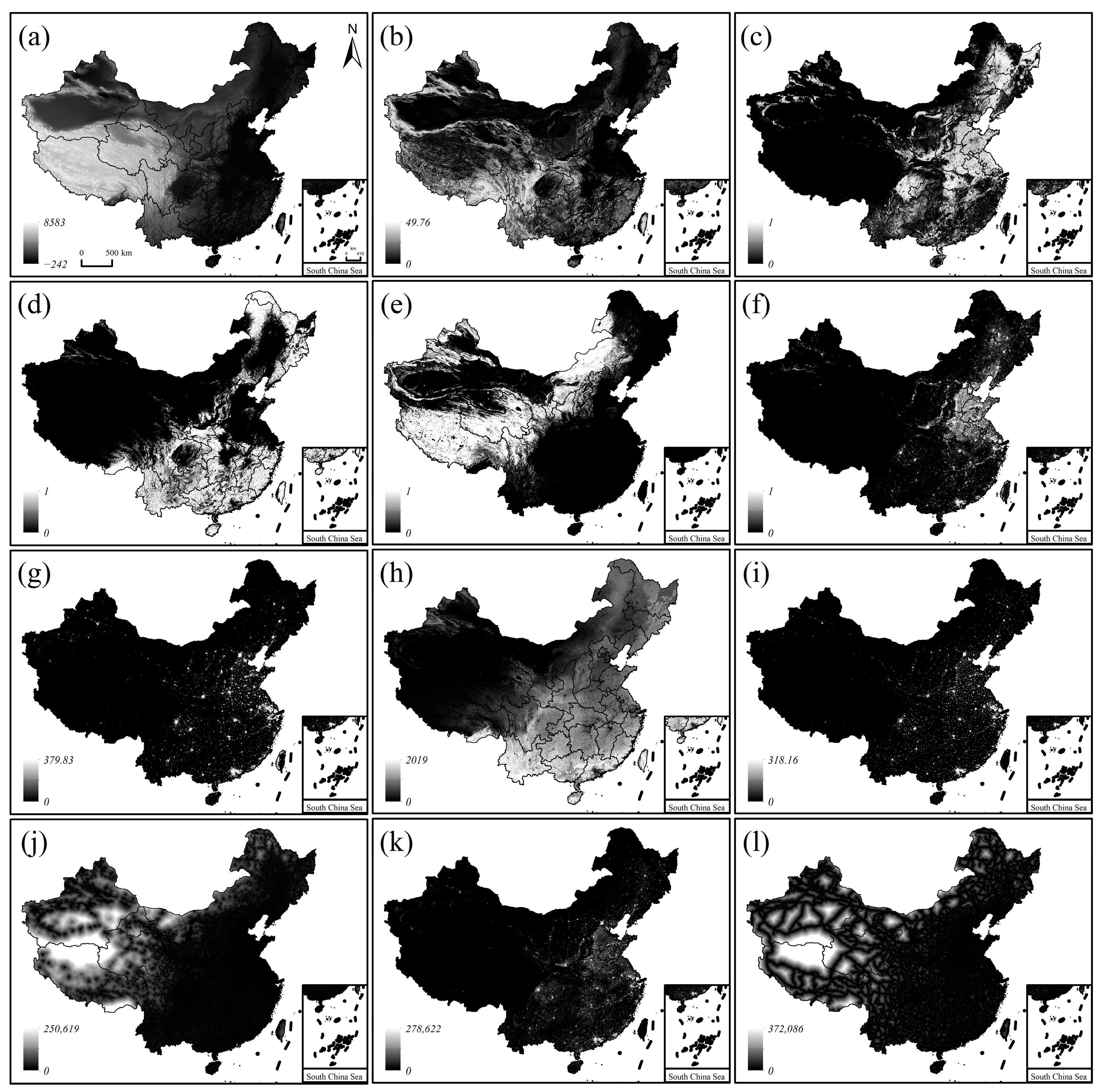
The datasets used in this paper contain China’s county-level GDP statistical data and auxiliary data. The auxiliary data mainly include NTL, land cover, population density, net primary productivity of vegetation (NPP), DEM, POIs, and road data (Table 1). Based on these data, the gridded datasets of twelve auxiliary variables were generated (Figure A1), and the generation methods are introduced below (seen in Section 2.1.2 and Section 2.1.3). All datasets were projected in an Albers equal-area projection [36].

2.1.1. GDP Statistical Data and Boundary of Administrative Units

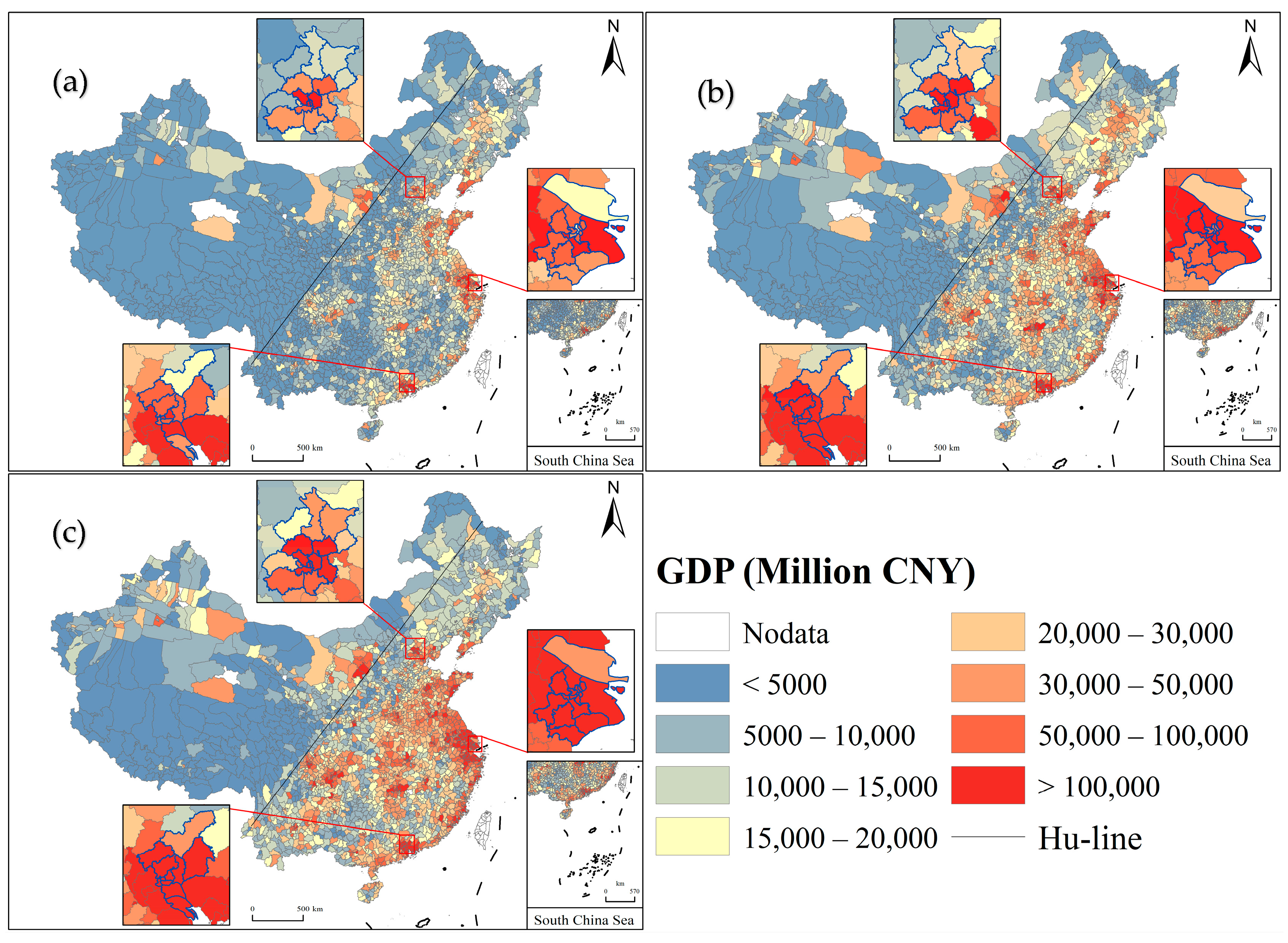
The GDP statistical data of counties in 2010, 2015, and 2020 in this paper are sourced from the China Statistical Yearbook for Regional Economy in 2011 and the China County Statistical Yearbook in 2016 and 2021, respectively. The GDP statistics of the municipal districts are from the municipal statistical yearbooks of 2011, 2016, and 2021. The GDP statistical data of Hong Kong, Macao, and Taiwan are missing, and the GDP statistics of Tianjin Binhai New Area were not included due to its abnormality. In total, 2767, 2835, and 2793 GDP statistical data at the county level were collected in 2010, 2015, and 2020, respectively. Due to the changes in a few county-level administrative units over the past decade, adjustments were made according to the information on the changes in administrative units in China from 2010 to 2020 (available at http://www.xzqh.org (accessed on 10 May 2023)). Finally, the GDP statistical data at the county level in 2010, 2015, and 2020 were linked to the corresponding administrative units (Figure A2).

2.1.2. Grid Data

Nighttime light intensity data are derived from the extended time series NPP-VIIRS-like NTL data [37]. The dataset provides nighttime light information with a spatial resolution of 1 km × 1 km from 2000 to 2020, which has been widely employed to assess and analyze the dynamics of population and socioeconomic development [40]. The China land cover dataset (CLCD) contains nine land cover types (farmland, forest, shrub, grassland, water, snow, barren, impervious, and wetland) with a spatial resolution of 30 m per year from 1990 to 2020 [38]. Four land cover types were selected to model GDP distribution, including farmland, forest, grassland, and impervious areas. In order to reduce the information loss of data in the resampling process, we produced the percentage data of land cover types with a resolution of 1 km × 1 km according to a previous study [41]. The digital elevation model (DEM) data and population density data were resampled to a spatial resolution of 1 km × 1 km using bilinear algorithms [42], and the slope data were obtained based on DEM data. Furthermore, the publicly published GDP-gridded data in 2010, 2015, and 2019, generated by Xu [43] (hereinafter referred to as Xu_GDP gridded data), were downloaded from the resource and environment database of the Chinese Academy of Sciences. These gridded data were developed by the multifactor weight distribution method with the data of land cover types, human settlements, and NTL. The multifactor weight distribution method calculates and standardizes the weight values of each factor, then calculates the total weight value [43]. These gridded data were used for comparative analysis of model accuracy.

2.1.3. POI Data

Point-of-interest (POI) data represent typical geospatial big data and are considered important for studying economic activities. POI data record the geographic locations of companies, education services, commercial houses, governments, and other elements. We initially performed data cleaning on the POI data (e.g., screening, deduplication, and sorting) [44]. A density analysis was then performed. The optimal bandwidth varies for different categories of POI. To determine the optimal bandwidth for each category of POI data, this paper selected 1~5 km as the bandwidth range, calculated the kernel density of each category of POI at 1 km intervals each time, and generated a gridded layer with a spatial resolution of 1 km × 1 km. After fitting the GDP census and the kernel density data of each POI with different bandwidths using the GRF model (introduced in Section 2.2), the optimal bandwidth was determined according to the optimal R2 value. Based on the kernel density data of each POI category with the optimal bandwidth, the weight values were calculated according to the percentage increase in the meansquared error (%IncMSE) of each POI category obtained by the GRF model. Table 2 shows the optimal bandwidth, %IncMSE, and weight value of nine categories of POI data in 2010, 2015, and 2020. Finally, nine different categories of POI density gridded data were fused into new density gridded data [45], as shown in Formulas (1) and (2):
D c = i = 1 n D i W i
W i = % I n c M S E i i = 1 n % I n c M S E i
where n is the number of POI categories, D c denotes the grid value of the fused POI density, D i ( i = 1, 2, …, 9) denotes the grid value of the i th category of POI density, and W i represents the weight of the i th category of POI density. Furthermore, we also generated the distance of POIs according to the previous study [45].

2.2. Methods

2.2.1. Geographical Random Forest

A geographical random forest (GRF) is an extension of the classical RF [24]. RF is a machine learning method that integrates multiple classification and regression decision trees [46] and has been widely used to solve nonlinear problems [47]. RF can measure the performance of the model without cross-validation or setting up a test set, that is, 1/3 of the samples of each tree that are not involved in training are used to estimate the mean square error (MSE) of OOB, and the performance index of OOB R2. The model can calculate the %IncMSE of each auxiliary variable, which is used to evaluate the importance of auxiliary variables. The larger the value of %IncMSE, the greater the contribution of the auxiliary variable to the model [48].
The classical RF is a nonspatial model, which makes it difficult to deal with the problem of spatial heterogeneity. Based on the theory of the GWR model, Georganos et al. [24] proposed a GRF model by extending the random forest model to a combination of multiple local submodels in space. Specifically, the GRF model generates a spatial weight matrix by introducing the spatial information of observation points and then integrates it with RF into a local regression analysis framework [49]. When dealing with spatial heterogeneity, GRF not only improves the prediction performance of traditional RF models but also helps to explore the coupling relationship between dependent variables and environmental variables in local space. Each local submodel calculates the %IncMSE of each environmental variable, which can reflect the spatial heterogeneity of the importance score of each variable. The maximum distance between the observation point and the kernel is called the bandwidth. Given the large differences in areas of county administrative units in China, the adaptive kernel is chosen [24], and the bi-square kernel function is selected as the weight kernel function, as shown in Formula (3):
w i j = 1 d i j b 2 2 ,   | d i j < b 0 ,   | d i j b
in which w i j is the weight of the observation point, d i j is the distance from the observation point to the submodel, and b represents the bandwidth.
The geographical random forest model employs the spatial weight matrix to adjust the sampling weight of samples in each local RF, as shown in Formula (4):
W = W 1 W 2 W i W n = w 11 w 12 w 1 n w 21 w 22 w 2 n w i 1 w i 2 w i n w n 1 w n 2 w n n ,    i 1,2 , , n
The equation of the classical RF regression is simplified as shown in Formula (5):
Y i = a x i + e
where Y i is the county GDP value of the ith observation point, a x i is a nonlinear prediction of RF based on a set of auxiliary variables, x, and e is the residual error.
GRF extends Formula (5) to use a subset of the original dataset each time, as shown in Formula (6):
Y i = a u i , v i x i + e
where a u i , v i is the prediction of the RF model calibrated at the position of sample i, and u i , v i is the coordinate of sample i.
The basic steps of geographical random forest are as follows: (1) The distance matrix between samples is calculated, and then the weight matrix is calculated using the bi-square kernel function according to the bandwidth parameters. (2) We input the ith sample, the neighborhood samples with sampling weight larger than 0, and their respective sampling weights, then, we train the ith local RF and calculate the variable importance until all local RFs have been trained. (3) The environmental variables and coordinates are inputted to calculate the distance matrix based on the coordinates. We then select the nearest local RF model for prediction and output the predicted GDP weights. In this paper, the R package SpatialML is used, and more information can be found in Kalogirou [50] and Georganos et al. [24,51].

2.2.2. GDP Density Mapping

Census GDP data were then disaggregated using a dasymetric mapping approach based on these weighting layers [52], as shown in Formula (7):
G D P g r i d = G D P c o u n t y × W g r i d W c o u n t y
where G D P g r i d denotes the GDP pixel value, G D P c o u n t y denotes the GDP statistic value of the county, W g r i d denotes the pixel value of GDP weight, and W c o u n t y represents the sum of the pixel values of the county’s GDP weight.

2.2.3. Accuracy Assessment

The determination coefficient (R2), root-mean-square error (RMSE), and mean absolute error (MAE) are used to evaluate the simulation effect of the GDP density weight layer, as shown in Formulas (8)–(10):
R 2 = i = 1 n ( Y c , i Y ¯ c ) Y e , i Y ¯ e i = 1 n Y c , i Y ¯ c 2 i = 1 n Y e , i Y ¯ e 2 2
M A E = 1 n i = 1 n | Y c , i Y e , i |
R M S E = 1 n i = 1 n Y c , i Y e , i 2
where n is the number of counties, Y c , i is the statistical value of the i th county, Y e , i is the weight value of the prediction of the i th county, and Y ¯ c and Y ¯ e are the averaged value of the GDP statistical data and the prediction.
Due to the lack of GDP statistical indicators at the township level, this paper compared the predicted GDP density weight value with the GDP statistical data, and then compared the modified GDP density maps with the publicly available Xu_GDP maps, in order to evaluate the rationality of the new GDP-gridded data.

2.2.4. Spatial Barycenter Model

The spatial barycenter model is a useful tool in visually and accurately tracing the process of spatial change in geographic elements [53]. We employed this model to explore the spatial changes in China’s GDP. The economic barycenter is calculated as shown in Formula (11):
X = i = 1 n M i X i i = 1 n M i , Y = i = 1 n M i Y i i = 1 n M i
where X and Y represent the coordinate of the economic barycenter, X i and Y i represent the coordinate of the i th grid of GDP density, respectively, and M i represents the value of the i th grid of GDP density.
The moving distance of the economic barycenter is calculated as shown in Formula (12):
D S k = Y s Y k 2 + X S X k 2
where D s k denotes the distance of the economic barycenter moving between two different years ( s and k) and ( X s , Y s )   a n d   ( X k , Y k ) denote the coordinate of economic barycenter in the sth year and kth year, respectively. In this study, we converted gridded data from three periods into point data using ArcGIS software and then conducted a spatial barycenter analysis of China’s GDP density from 2010 to 2020.

3. Results

3.1. Multitemporal GDP Density Maps

The GRF model, used to predict China’s GDP density, has a consistently high variance explained for 2010, 2015, and 2020, with values of 95.73%, 95.86%, and 96.61%, respectively. Further assessments show that the GDP density weight and GDP census data at the county level in 2010, 2015, and 2020 are highly consistent, with R2 values of 0.79, 0.79, and 0.75, and MAE values of 4.91 × 10⁶, 8.02 × 10⁶, and 12.97 × 10⁶, respectively (Figure 1).
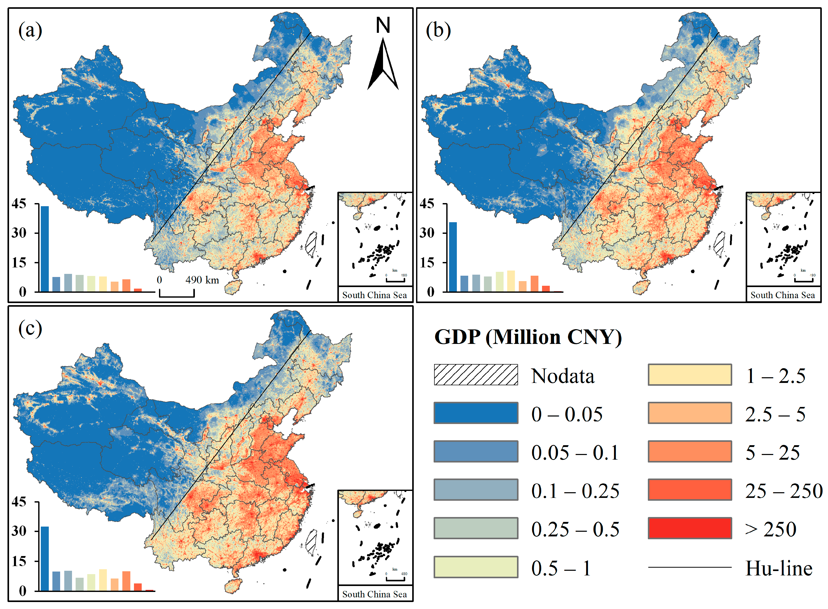
Our GDP density maps finely depict the spatial pattern of China’s GDP distribution, which is high in the southeast and low in the northwest (Figure 2). According to the GDP density classification in previous studies [8,10], we found that the areas with a GDP density below 0.1 million CNY/km2 account for about half of China (Table 3), mainly distributed in grassland and desert areas in the northwest side of the Hu-line. The areas with a GDP density higher than 5 million CNY/km2 account for about one-tenth of China, mainly distributed in urban agglomerations such as the Pearl River Delta and Yangtze River Delta. The proportion of the areas below 0.05 million CNY/km2 decreased from 43.82% in 2010 to 32.44% in 2020, with a decrease of 8.32% and 3.06% in the first and second five-year periods, respectively. The proportion of the areas above 1 million CNY/km2 increased from 22.11% in 2010 to 32.22% in 2020, with an increase of 6.74% and 3.37% in the first and second five-year periods, respectively. Moreover, the proportion of the areas above 25 million CNY/km2 increased from 2.21% in 2010 to 4.68% in 2020, with an increase of more than 100%. These results showed that China’s GDP density shows a trend of continuous increase in the proportion of medium and rich areas and a rapid decrease in the proportion of poor areas.

3.2. Spatiotemporal Changes in GDP Density

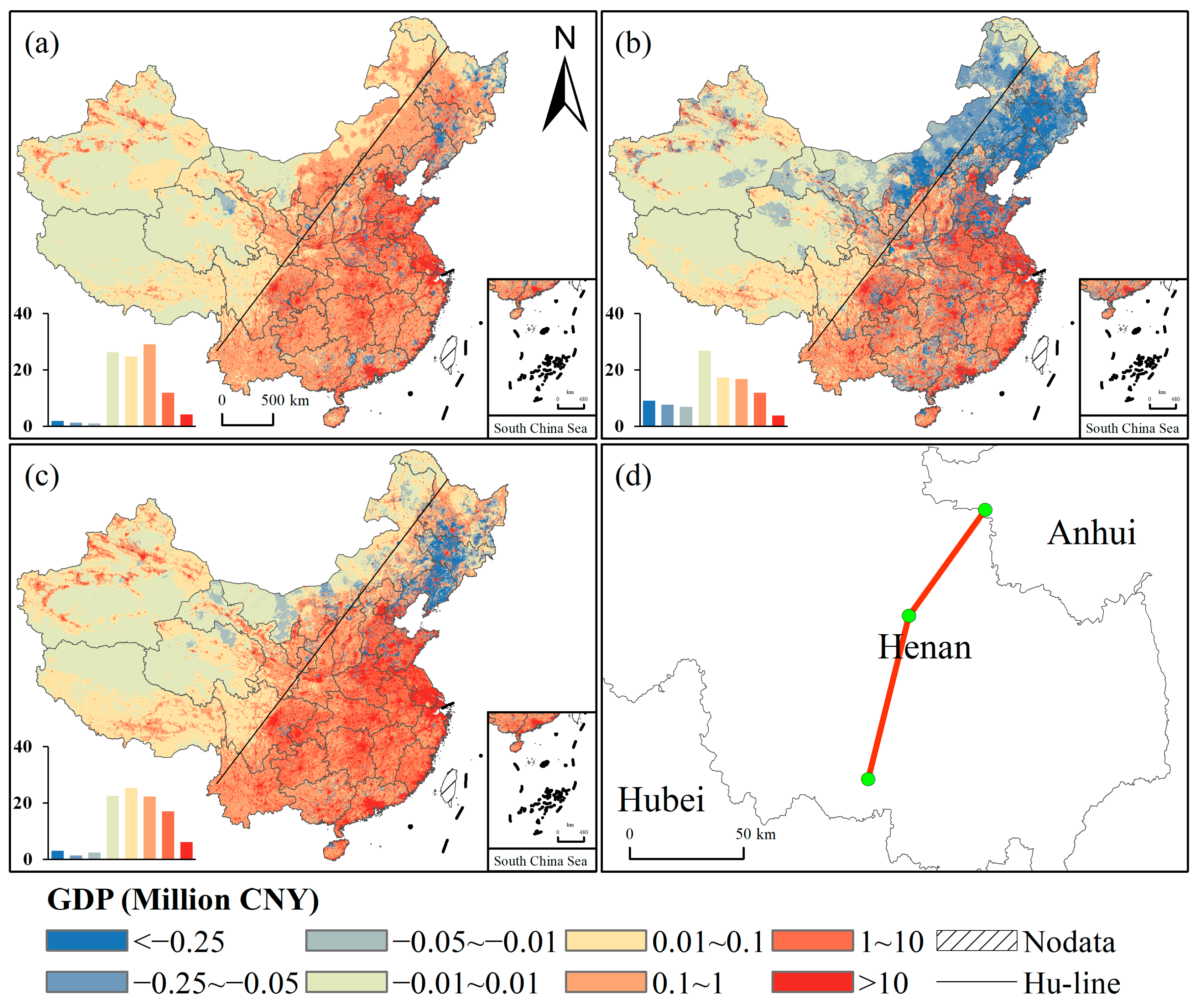
China’s GDP increased from 2010 to 2020 overall. The areas with an increase and decrease of 0.01 million CNY/km2 account for 70.73% and 6.77% of China, respectively (Figure 3c and Table 4). Spatially, GDP density in central and southern China and nondesert regions in western China showed a significant increase, while GDP density in some areas in northeast China declined to a certain extent.
The changes in GDP density both during 2010–2015 and 2015–2020 display spatial heterogeneity (Figure 3a,b). The areas where GDP density increased by more than 0.1 million CNY/km2 in the five years before and after account for 45.10% and 32.38% of China, respectively (Table 4), with the former being approximately 1.4 times the latter. The former is primarily distributed in the southeast side of the Hu-line, while the latter is mainly concentrated in southeast China and urban agglomerations. Furthermore, the area with GDP declining by more than 0.01 million CNY/km2 in the five years before and after 2015 accounts for 4.03% and 23.58% of China, respectively. The latter is approximately six times the former, mainly in the rural areas of northeast China and parts of north China.
The result showed that barycenters of China’s GDP moved 128.80 km to the southwest in the past decade (Figure 3d). The barycenters of China’s GDP shifted 57.33 km to the southwest in 2010–2015 and continued to move 73.78 km to the south and west in 2015–2020, that is, from the northwestern edge of Anhui Province to the southwest to the border area between Henan Province and Hubei Province. The moving trajectory of barycenters of China’s GDP was dominated by sustainable development in southeast China, the rise of central China, and the economic recession in northeast China, (Figure 3). These results indicated that the phenomenon of the shift from “strong north and weak south” to “strong south and weak north” was enhanced.

3.3. Regional Difference of Random Forest Variable Importance

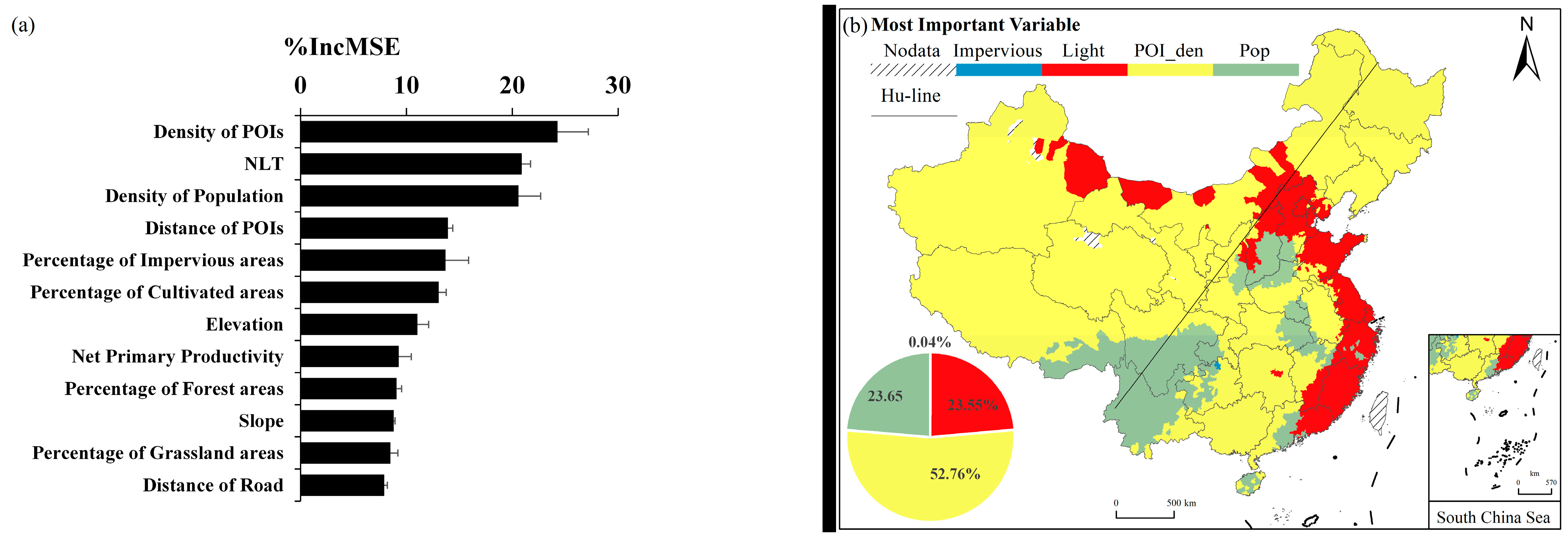
Among the twelve auxiliary variables, the mean value of the %IncMSE in the GRF model showed that POI density, NLT, and population density ranked in the top three. The value of the %IncMSE of human environment variables was generally higher than that of the natural environment variables (Figure 4a). POI density, NLT, and population density reflect spatial aggregation and regional differences of labor, resources, and capital in detail, which is beneficial for capturing the spatial differences of GDP. The spatial distribution of the variables with the highest importance scores of each submodel is shown in Figure 4b. The number of counties with the highest importance score of POI density in GDP mapping accounts for 52.78% of total counties, while those for population density and NTL accounted for 23.66% and 23.56%, respectively. The areas with the highest importance score of NLT to GDP are concentrated in the coastal provinces from Hebei to Guangdong, while the areas with the highest importance score of population density are mainly located in southwest China (e.g., Yunnan Province and southern Sichuan Province) and central north China (e.g., southwestern Shanxi Province). These results suggest that POI density, NLT, and population density are the three key auxiliary variables that affect the spatial distribution of GDP density, and they show obvious spatial heterogeneity.
The spatial distribution of the importance score of the twelve auxiliary variables is shown in Figure 5. The %IncMSE values of twelve variables show regional differences, indicating spatial heterogeneity in the relationship between the auxiliary variable and GDP density. Specifically, the importance scores of POI density, NLT, and population density were generally greater than 15. Among them, the importance score of POI was high in northwest China and low in southeast China, while the importance score of population density was high in western China and low in eastern China. The importance scores of natural environmental variables such as slope, elevation, NPP, and proportion of forest area are relatively low. The importance score of both the proportion of forest area and NPP were high in the southeast and low in the northwest.

4. Discussion

4.1. Comparison with the Open Access Gridded GDP Datasets

The determination coefficient (R2) for the GDP density simulated by GRF and the county statistical value reached or exceeded 0.75 (Figure 1). In previous studies of county population spatialization, an R2 value of 0.70 or higher indicates that the spatial characteristics of population density can be described well [54,55], which to some extent indicates the feasibility of our spatialized GDP results.
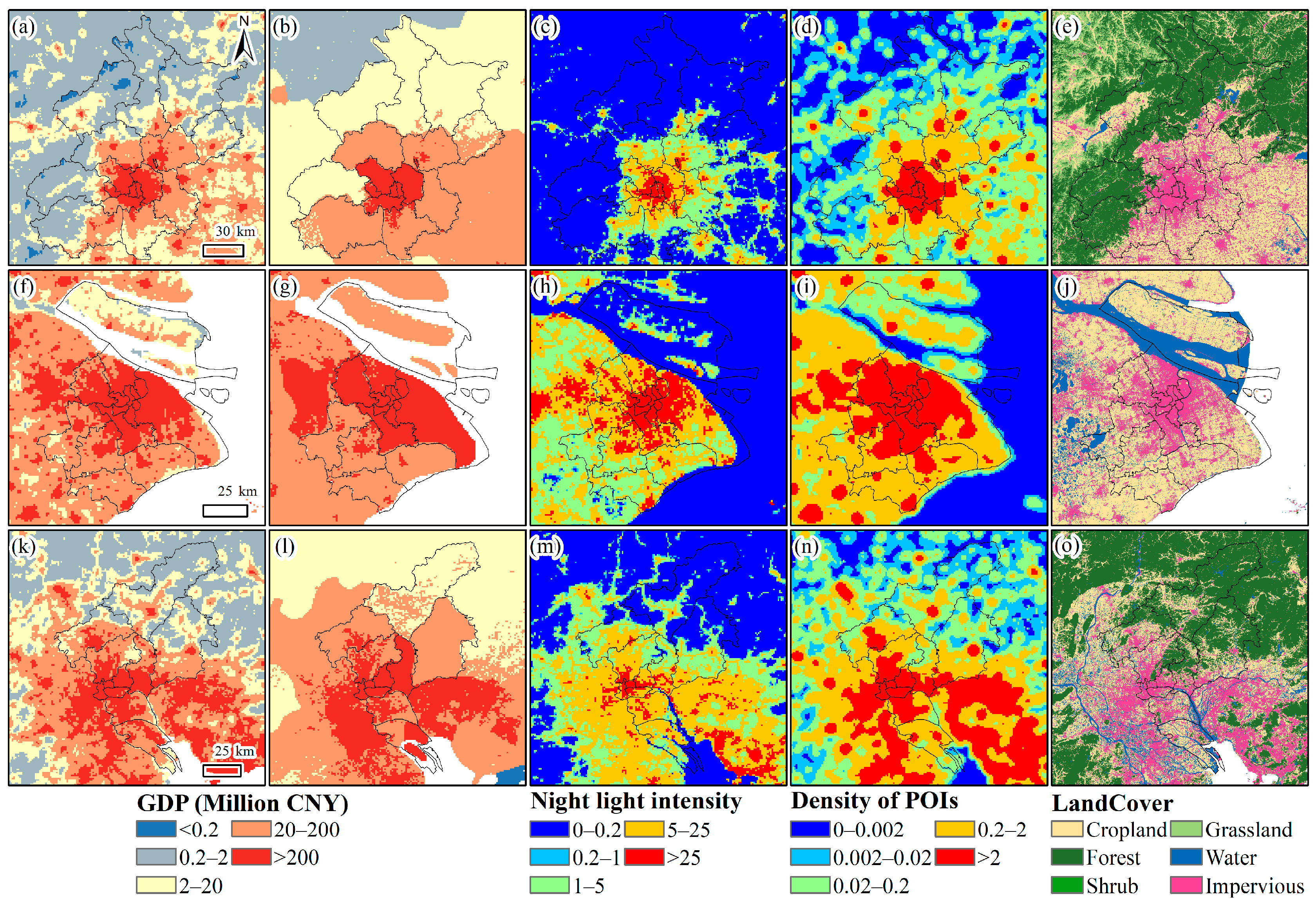
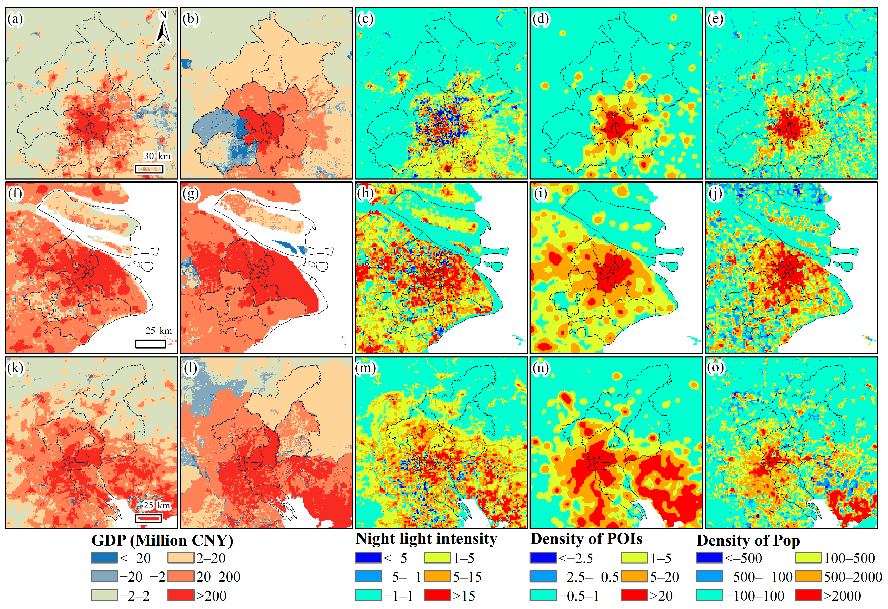
This study generated multitemporal GDP density maps based on the geographical random forest and multisource data. Here, we compared them with the publicly available Xu_GDP gridded data, taking Beijing, Shanghai, and Guangzhou in 2015 as examples (Figure 6). In terms of the spatial distribution of GDP, the two gridded data show obvious clusters of GDP in urban areas, while our new maps depict more detailed differences within the administrative units at the county level, avoiding overestimation in nonurban areas. These phenomena benefit from the advantage of the geographical random forest’s ability to capture the complex relationship between GDP and POI, NLT, land cover, and other auxiliary variables. Furthermore, in terms of the spatial pattern of the changes in GDP from 2010 to 2020, our new GDP maps also accurately depicted the spatial differences in changes in GDP density within the administrative units at the county level and were consistent with changes in NLT, POI density, and population density (Figure 7).

4.2. Change in GDP Density over the Past Decades

In 2020, the areas with a GDP density below 0.05 million CNY/km2 comprised approximately 1/3 of China, mainly located in remote mountainous regions with sparse populations and vast wilderness. Compared to their extent in 2010, these areas experienced an 11.38% reduction (Figure 2 and Table 3). (Figure 2 and Table 3). Over the past decade, areas experiencing an increase of 0.01 million CNY/km2 in GDP density account for more than 2/3 of China (Figure 3a and Table 4). These results are a great achievement, as China has insisted on comprehensive poverty alleviation and focused on the implementation of the rural revitalization strategy [56]. Meanwhile, in 2020, areas with a GDP density higher than 25 million CNY/km2 accounted for 4.68% of China. These areas mainly comprised urban agglomerations such as Beijing, Shanghai, Guangzhou, and Shenzhen, as well as prefecture-level cities, and their GDP density nearly doubled compared to that in 2010. This is related to China actively promoting the urbanization process, especially for the urban agglomerations [57].
The areas with a GDP density increase of more than 0.1 million CNY/km2 during 2010–2015 are 1.4 times greater than those during 2015–2020, reflecting the general background of a continued slowdown in China’s economic growth, that is, from approximately 10% to 6.1% in 2019 compared with the previous decade [53]. Meanwhile, the GDP in some rural areas of northeast China and parts of northern China declined from 2015 to 2020, accounting for approximately a quarter of China. This phenomenon may be related to the changing demographics of China’s rural population, as well as ecological environmental protection and construction efforts, such as reforestation projects [53,58,59]. The 2020 census data showed that the northeastern region has experienced population shrinkage, especially in rural areas [60]. In addition, the growth rate of the old industrial bases in northeast China has declined, and the radiating and leading roles of large cities in influencing surrounding small and medium-sized towns are limited [53]. The potential reasons for the decline in GDP density in these regions should be further explored, to prevent poverty from returning.
Over the past decade, the economic gravity center shifted southwestward by 128.80 km (Figure 3d). This is consistent with the existing result based on provincial GDP in terms of direction [53]; however, the distance moved is approximately twice as far as the latter, which is likely due to the use of refined GDP-gridded data in our study. As China’s economy continues to grow, the widening gaps between the South and the North [53] suggest that regional development imbalances might become a pressing issue for China in the future [61].

4.3. Regional Differences in Random Forest Variable Importance

POI density ranks first in the importance score in the GRF model, and the proportion of counties with the highest importance score of POI density to GDP mapping is 52.78% (Figure 4), which reflects the key role of POI data in GDP spatialization [18]. This is followed by NLT and population density, accounting for 23.56% and 23.66%, respectively. Accelerating the flow of production factors and concentrating production factors help promote economic development. The former is concentrated in the eastern coastal provinces of China. This concentration is related to the development and opening policy tilted toward the coastal areas in the last 40 years, which is likely related to the obvious difference between urban and nonurban power facilities [61]. These results show that the relationship between GDP density and key auxiliary variables exhibits spatial heterogeneity, necessitating the integration of multisource data in GDP spatialization.

4.4. Limitation and Future Work

The reliability of spatialized GDP results depends heavily on the quality of statistical data, while a little GDP statistical data at the county level may contain errors, likely due to intentional manipulation [5]. Meanwhile, we did not take into account the Black Swan event in 2020—the COVID-19 pandemic—which led to slower GDP growth rates compared to other years, especially for Hubei Province. Hence, it might have a negative effect on the result of the spatial pattern of the change in GDP density during 2010–2020. The selected indicators may not apply to some resource-based cities, which brings uncertainty to the spatial distribution of GDP density in these cities. Additionally, to the best of our knowledge, the POI dataset can be traced back to 2012, and no earlier dataset has been published publicly. Meanwhile, the POI dataset might not be complete in remote areas in the year 2012, while it might be more abundant in the year 2020, which also brings uncertainties to the analysis of the change in GDP density.
A recent study noted that new geospatial big data (e.g., Tencent user density (TUD) data) is a promising data source for mapping GDP density [8]; more attention should be paid to integrating multisource geospatial big data to further improve the precision of multitemporal GDP mapping in future work. Furthermore, even though our maps are seasonable and acceptable, the GRF is a shallow machine learning method. Recent studies pointed out that deep learning performs better in generating population grid data than shallow machine learning [62]. A geographically deep learning model was used to downscale land surface temperature and water quality [63,64], suggesting the potential to map GDP density using a geographical deep learning model.

5. Conclusions

We mapped China’s GDP distribution using GRF based on remotely sensed and POI data in 2010, 2015, and 2020. Our new maps finely depict the spatial pattern of China’s GDP distribution, which mirrors China’s achievements in alleviating poverty and the widening gaps between the South and North. The proportion of areas with GDP density lower than 0.05 million CNY/km2 decreased by 11.38% over the past decade, while that higher than 1 million CNY/km2 increased by 11.11%. The areas with an increase of 0.01 million CNY/km2 account for more than 2/3 of China, while the GDP density of nonurban areas in northeast China declined, especially between 2015 and 2020. The spatial barycenter analysis further showed that the barycenter of China’s GDP had moved to the southwest. Meanwhile, the relationships between GDP density and auxiliary variables exhibit spatial heterogeneity. The number of counties with the highest importance score of POI density in GDP mapping accounts for 52.78% of the total number of counties, while population density and NTL accounted for 23.66% and 23.56%, respectively. Spatially, the counties with the highest importance score of population density to GDP mapping are primarily distributed in the southwest and central north China, and those for NTL in GDP mapping are mainly located in the coastal provinces. These indicate that spatial differences in the relationship between GDP and auxiliary variables should be taken into account in the current models of GDP mapping.

Author Contributions

Conceptualization and methodology, F.L.; writing—original draft preparation, F.D. and L.C.; software, L.C.; writing—review and editing, L.L., L.C., W.M., W.L., Y.C. and C.P. All authors have read and agreed to the published version of the manuscript.

Funding

This research was funded by the Natural Science Foundation of Fujian Province of China (Grant No. 2020J05233) and the National Natural Science Foundation of China (Grant No. 42101099).

Institutional Review Board Statement

Not applicable.

Informed Consent Statement

Not applicable.

Data Availability Statement

Not applicable.

Acknowledgments

We sincerely thank Qian Chen from Zhejiang University for the valuable feedback.

Conflicts of Interest

The authors declare no conflict of interest.

Appendix A

Figure A1. Spatial pattern of the twelve auxiliary variables in 2020: (a) elevation, (b) slope, (c) the percentage of cultivated areas, (d) the percentage of forest areas, (e) the percentage of grassland areas, (f) the percentage of impervious areas, (g) night-light intensity, (h) net primary productivity, (i) density of POIs, (j) distance of POIs, (k) density of population, and (l) distance of the road.
Sustainability 15 08062 g0a1
Figure A2. Maps of the GDP statistical data at the county level in (a) 2010, (b) 2015, and (c) 2020.
Sustainability 15 08062 g0a2

References

  1. Geiger, T. Continuous national gross domestic product (GDP) time series for 195 countries: Past observations (1850–2005) harmonized with future projections according to the shared socio-economic pathways. Earth Syst. Sci. Data 2018, 10, 847–856. [Google Scholar] [CrossRef]
  2. Henderson, J.V.; Storeygard, A.; Weil, D.N. Measuring Economic Growth from Outer Space. Am. Econ. Rev. 2012, 102, 994–1028. [Google Scholar] [CrossRef] [PubMed]
  3. Sun, J.; Di, L.; Sun, Z.; Wang, J.; Wu, Y. Estimation of GDP Using Deep Learning With NPP-VIIRS Imagery and Land Cover Data at the County Level in CONUS. IEEE J. Sel. Top. Appl. Earth Obs. Remote Sens. 2020, 13, 1400–1415. [Google Scholar] [CrossRef]
  4. Wang, X.; Sutton, P.C.; Qi, B. Global Mapping of GDP at 1 km2 Using VIIRS Nighttime Satellite Imagery. Isprs Int. J. Geo-Inf. 2019, 8, 580. [Google Scholar] [CrossRef]
  5. Chen, X.; Nordhaus, W.D. Using luminosity data as a proxy for economic statistics. Proc. Natl. Acad. Sci. USA 2011, 108, 8589–8594. [Google Scholar] [CrossRef]
  6. Li, R.; Shan, Y.; Bi, J.; Liu, M.; Ma, Z.; Wang, J.; Hubacek, K. Balance between poverty alleviation and air pollutant reduction in China. Environ. Res. Lett. 2021, 16, 94019. [Google Scholar] [CrossRef]
  7. Wang, Y.P.; Zhou, X.N. The year 2020, a milestone in breaking the vicious cycle of poverty and illness in China. Infect. Dis. Poverty 2020, 9, 11. [Google Scholar] [CrossRef]
  8. Chen, Y.; Wu, G.; Ge, Y.; Xu, Z. Mapping Gridded Gross Domestic Product Distribution of China Using Deep Learning With Multiple Geospatial Big Data. IEEE J. Sel. Top. Appl. Earth Obs. Remote Sens. 2022, 15, 1791–1802. [Google Scholar] [CrossRef]
  9. Huang, Z.; Li, S.; Gao, F.; Wang, F.; Lin, J.; Tan, Z. Evaluating the performance of LBSM data to estimate the gross domestic product of China at multiple scales: A comparison with NPP-VIIRS nighttime light data. J. Clean Prod. 2021, 328, 129558. [Google Scholar] [CrossRef]
  10. Chen, Q.; Hou, X.; Zhang, X.; Ma, C. Improved GDP spatialization approach by combining land-use data and night-time light data: A case study in China’s continental coastal area. Int. J. Remote Sens. 2016, 37, 4610–4622. [Google Scholar] [CrossRef]
  11. GUO, H.; ZHU, W. A review on the spatial disaggregation of socioeconomic statistical data. Acta Geogr. Sin. 2022, 77, 2650–2667. [Google Scholar]
  12. Elvidge, C.D.; Baugh, K.E.; Kihn, E.A.; Kroehl, H.W.; Davis, E.R.; Davis, C.W. Relation between satellite observed visible-near infrared emissions, population, economic activity and electric power consumption. Int. J. Remote Sens. 1997, 18, 1373–1379. [Google Scholar] [CrossRef]
  13. Doll, C.N.H.; Muller, J.; Morley, J.G. Mapping regional economic activity from night-time light satellite imagery. Ecol. Econ. 2006, 57, 75–92. [Google Scholar] [CrossRef]
  14. Li, X.; Xu, H.; Chen, X.; Li, C. Potential of NPP-VIIRS Nighttime Light Imagery for Modeling the Regional Economy of China. Remote Sens. 2013, 5, 3057–3081. [Google Scholar] [CrossRef]
  15. Shi, K.; Yu, B.; Huang, Y.; Hu, Y.; Yin, B.; Chen, Z.; Chen, L.; Wu, J. Evaluating the Ability of NPP-VIIRS Nighttime Light Data to Estimate the Gross Domestic Product and the Electric Power Consumption of China at Multiple Scales: A Comparison with DMSP-OLS Data. Remote Sens. 2014, 6, 1705–1724. [Google Scholar] [CrossRef]
  16. Zhao, N.; Liu, Y.; Cao, G.; Samson, E.L.; Zhang, J. Forecasting China’s GDP at the pixel level using nighttime lights time series and population images. GIScience Remote Sens. 2017, 54, 407–425. [Google Scholar] [CrossRef]
  17. Sutton, P.C.; Costanza, R. Global estimates of market and non-market values derived from nighttime satellite imagery, land cover, and ecosystem service valuation. Ecol. Econ. 2002, 41, 509–527. [Google Scholar] [CrossRef]
  18. Chen, Q.; Ye, T.; Zhao, N.; Ding, M.; Ouyang, Z.; Jia, P.; Yue, W.; Yang, X. Mapping China’s regional economic activity by integrating points-of-interest and remote sensing data with random forest. Environ. Plan. B Urban Anal. City Sci. 2021, 48, 1876–1894. [Google Scholar] [CrossRef]
  19. Zhao, M.; Cheng, W.; Zhou, C.; Li, M.; Wang, N.; Liu, Q. GDP Spatialization and Economic Differences in South China Based on NPP-VIIRS Nighttime Light Imagery. Remote Sens. 2017, 9, 673. [Google Scholar] [CrossRef]
  20. Huang, Z. Chinese GDP Modeling and Simulating Based Onremote Sensing and Social Perception Data at Multiple Scales. Master’s Thesis, Guangzhou University, Guangzhou, China, 2022. [Google Scholar]
  21. Achten, S.; Lessmann, C. Spatial inequality, geography and economic activity. World Dev. 2020, 136, 105114. [Google Scholar] [CrossRef]
  22. Li, C.; Huo, Z.; Wang, X.; Wu, Y. Study on spatio-temporal modelling between NPP-VIIRS night-time light intensity and GDP for major urban agglomerations in China. Int. J. Remote Sens. 2022, 44, 1–24. [Google Scholar] [CrossRef]
  23. Liu, H.; Jiang, D.; Yang, X.; Luo, C. Spatialization Approach to 1 km Grid GDP Supported by Remote Sensing. Geo-Inf. Sci. 2005, 7, 120–123. [Google Scholar]
  24. Georganos, S.; Grippa, T.; Niang Gadiaga, A.; Linard, C.; Lennert, M.; Vanhuysse, S.; Mboga, N.; Wolff, E.; Kalogirou, S. Geographical random forests: A spatial extension of the random forest algorithm to address spatial heterogeneity in remote sensing and population modelling. Geocarto Int. 2021, 36, 121–136. [Google Scholar] [CrossRef]
  25. Khan, S.N.; Li, D.; Maimaitijiang, M. A Geographically Weighted Random Forest Approach to Predict Corn Yield in the US Corn Belt. Remote Sens. 2022, 14, 2843. [Google Scholar] [CrossRef]
  26. Li, L.; Huang, C.; Zhang, Y.; Liu, L.; Wang, Z.; Zhang, H.; Ding, M.; Huamin, Z. Mapping the multi-temporal grazing intensity on the Qinghai-Tibet Plateau using geographically weighted random forest. Scientia Geogr. Sin. 2023, 43, 398–410. [Google Scholar]
  27. Lotfata, A.; Georganos, S.; Kalogirou, S.; Helbich, M. Ecological Associations between Obesity Prevalence and Neighborhood Determinants Using Spatial Machine Learning in Chicago, Illinois, USA. Isprs. Int. J. Geo-Inf. 2022, 11, 550. [Google Scholar] [CrossRef]
  28. Luo, Y.; Yan, J.; McClure, S.C.; Li, F. Socioeconomic and environmental factors of poverty in China using geographically weighted random forest regression model. Environ. Sci. Pollut. Res. 2022, 29, 33205–33217. [Google Scholar] [CrossRef]
  29. Quiñones, S.; Goyal, A.; Ahmed, Z.U. Geographically weighted machine learning model for untangling spatial heterogeneity of type 2 diabetes mellitus (T2D) prevalence in the USA. Sci. Rep. 2021, 11, 6955. [Google Scholar] [CrossRef]
  30. Grekousis, G.; Feng, Z.; Marakakis, I.; Lu, Y.; Wang, R. Ranking the importance of demographic, socioeconomic, and underlying health factors on US COVID-19 deaths: A geographical random forest approach. Health Place 2022, 74, 102744. [Google Scholar] [CrossRef]
  31. China The State Council Information Office of the People’s Republic of China. Poverty Alleviation: China’s Experience and Contribution. In Beijing. 2021. Available online: http://www.scio.gov.cn/zfbps/ndhf/44691/Document/1701663/1701663.htm (accessed on 10 May 2023).
  32. WorldBank The World Bank 2020 World Bank Country and Lending Groups. Available online: https://datahelpdesk.worldbank.org/knowledgebase/articles/906519-world-bank-country-andlending-groups (accessed on 10 May 2023).
  33. Chen, J.; Gao, M.; Cheng, S.; Hou, W.; Song, M.; Liu, X.; Liu, Y. Global 1 km  ×  1 km gridded revised real gross domestic product and electricity consumption during 1992–2019 based on calibrated nighttime light data. Sci. Data 2022, 9, 202. [Google Scholar] [CrossRef]
  34. Kummu, M.; Taka, M.; Guillaume, J.H.A. Gridded global datasets for Gross Domestic Product and Human Development Index over 1990–2015. Sci. Data 2018, 5, 180004. [Google Scholar] [CrossRef]
  35. Gibson, J.; Boe-Gibson, G. Nighttime Lights and County-Level Economic Activity in the United States: 2001 to 2019. Remote Sens. 2021, 13, 2741. [Google Scholar] [CrossRef]
  36. Šavriǒ, B.; Jenny, B. Automating the selection of standard parallels for conic map projections. Comput. Geosci. 2016, 90, 202–212. [Google Scholar] [CrossRef]
  37. Chen, Z.; Yu, B.; Yang, C.; Zhou, Y.; Yao, S.; Qian, X.; Wang, C.; Wu, B.; Wu, J. An extended time series (2000–2018) of global NPP-VIIRS-like nighttime light data from a cross-sensor calibration. Earth Syst. Sci. Data 2021, 13, 889–906. [Google Scholar] [CrossRef]
  38. Yang, J.; Huang, X. The 30 m annual land cover dataset and its dynamics in China from 1990 to 2019. Earth Syst. Sci. Data 2021, 13, 3907–3925. [Google Scholar] [CrossRef]
  39. Tatem, A.J. WorldPop, open data for spatial demography. Sci. Data 2017, 4, 170004. [Google Scholar] [CrossRef]
  40. Ji, J.; Tang, Z.; Zhang, W.; Liu, W.; Jin, B.; Xi, X.; Wang, F.; Zhang, R.; Guo, B.; Xu, Z.; et al. Spatiotemporal and Multiscale Analysis of the Coupling Coordination Degree between Economic Development Equality and Eco-Environmental Quality in China from 2001 to 2020. Remote Sens. 2022, 14, 737. [Google Scholar] [CrossRef]
  41. Li, L.; Zhang, Y.; Liu, L.; Wang, Z.; Zhang, H.; Li, S.; Ding, M. Mapping Changing Population Distribution on the Qinghai–Tibet Plateau since 2000 with Multi-Temporal Remote Sensing and Point-of-Interest Data. Remote Sens. 2020, 12, 4059. [Google Scholar] [CrossRef]
  42. Polidori, L.; Chorowicz, J. Comparison of bilinear and Brownian interpolation for digital elevation models. Isprs J. Photogramm. 1993, 48, 18–23. [Google Scholar] [CrossRef]
  43. Xu, X.; China GDP Spatial Distribution Kilometre Grid Dataset. Resource and Environmental Science Data Registration and Publishing System. 2017. Available online: https://www.resdc.cn/DOI/doi.aspx?DOIid=33 (accessed on 10 May 2023).
  44. Wang, J.; Wei, J.; Zhang, W.; Liu, Z.; Du, X.; Liu, W.; Pan, K. High-resolution temporal and spatial evolution of carbon emissions from building operations in Beijing. J. Clean Prod. 2022, 376, 134272. [Google Scholar] [CrossRef]
  45. Ye, T.; Zhao, N.; Yang, X.; Ouyang, Z.; Liu, X.; Chen, Q.; Hu, K.; Yue, W.; Qi, J.; Li, Z.; et al. Improved population mapping for China using remotely sensed and points-of-interest data within a random forests model. Sci. Total Environ. 2019, 658, 936–946. [Google Scholar] [CrossRef] [PubMed]
  46. Breiman, L. Random Forests. Mach. Learn 2001, 45, 5–32. [Google Scholar] [CrossRef]
  47. Catani, F.; Lagomarsino, D.; Segoni, S.; Tofani, V. Landslide susceptibility estimation by random forests technique: Sensitivity and scaling issues. Nat. Hazard Earth Sys. 2013, 13, 2815–2831. [Google Scholar] [CrossRef]
  48. van der Laan, M.J. Statistical Inference for Variable Importance. Int. J. Biostat. 2006, 2, 2. [Google Scholar] [CrossRef]
  49. Luo, Y.; Yan, J.; McClure, S. Distribution of the environmental and socioeconomic risk factors on COVID-19 death rate across continental USA: A spatial nonlinear analysis. Environ. Sci. Pollut. Res. 2021, 28, 6587–6599. [Google Scholar] [CrossRef]
  50. Kalogirou, S.; Georganos, S. Package ‘SpatialML’. 2019. Available online: https://mran.microsoft.com/package/SpatialML (accessed on 10 May 2023).
  51. Georganos, S.; Kalogirou, S. A Forest of Forests: A Spatially Weighted and Computationally Efficient Formulation of Geographical Random Forests. Isprs. Int. J. Geo-Inf. 2022, 11, 471. [Google Scholar] [CrossRef]
  52. Liang, H.; Guo, Z.; Wu, J.; Chen, Z. GDP spatialization in Ningbo City based on NPP/VIIRS night-time light and auxiliary data using random forest regression. Adv. Space Res. 2020, 65, 481–493. [Google Scholar] [CrossRef]
  53. Liang, L.; Chen, M.; Luo, X.; Xian, Y. Changes pattern in the population and economic gravity centers since the Reform and Opening up in China: The widening gaps between the South and North. J. Clean Prod. 2021, 310, 127379. [Google Scholar] [CrossRef]
  54. Hui, L.; Hongsheng, Z.; Yinyi, L.; Shan, W.; Zhifeng, W. Spatiotemporal changes of gridded urban population in the Guangdong-Hong Kong-Macao Greater Bay Area based on impervious surface-population correlation. Prog. Geogr. 2018, 37, 1644–1652. [Google Scholar]
  55. Tan, M.; Li, X.; Li, S.; Xin, L.; Wang, X.; Li, Q.; Li, W.; Li, Y.; Xiang, W. Modeling population density based on nighttime light images and land use data in China. Appl. Geogr. 2018, 90, 239–247. [Google Scholar] [CrossRef]
  56. Li, Y.; Jia, L.; Wu, W.; Yan, J.; Liu, Y. Urbanization for rural sustainability—Rethinking China’s urbanization strategy. J. Clean Prod. 2018, 178, 580–586. [Google Scholar] [CrossRef]
  57. Gu, C.; Hu, L.; Cook, I.G. China’s urbanization in 1949–2015: Processes and driving forces. Chin. Geogr. Sci. 2017, 27, 847–859. [Google Scholar] [CrossRef]
  58. Chen, C.; Park, T.; Wang, X.; Piao, S.; Xu, B.; Chaturvedi, R.K.; Fuchs, R.; Brovkin, V.; Ciais, P.; Fensholt, R.; et al. China and India lead in greening of the world through land-use management. Nat. Sustain. 2019, 2, 122–129. [Google Scholar] [CrossRef]
  59. Song, Y.; Wang, Y.; Jin, L.; Shi, W.; Aryal, J.; Comber, A. Quantitative contribution of the Grain for Green Program to vegetation greening and its spatiotemporal variation across the Chinese Loess Plateau. Land Degrad. Dev. 2022, 33, 1878–1891. [Google Scholar] [CrossRef]
  60. Liu, T.; Peng, R.; Zhuo, Y.; Cao, G. China’s changing population distribution and influencing factors: Insights from the 2020 census data. Acta Geogr. Sin. 2022, 77, 381–394. [Google Scholar]
  61. Gu, Y.; Shao, Z.; Huang, X.; Cai, B. GDP Forecasting Model for China’s Provinces Using Nighttime Light Remote Sensing Data. Remote Sens. 2022, 14, 3671. [Google Scholar] [CrossRef]
  62. Zhao, S.; Liu, Y.; Zhang, R.; Fu, B. China’s population spatialization based on three machine learning models. J. Clean Prod. 2020, 256, 120644. [Google Scholar] [CrossRef]
  63. Wu, S.; Qi, J.; Yan, Z.; Lyu, F.; Lin, T.; Wang, Y.; Du, Z. Spatiotemporal assessments of nutrients and water quality in coastal areas using remote sensing and a spatiotemporal deep learning model. Int. J. Appl. Earth Obs. 2022, 112, 102897. [Google Scholar] [CrossRef]
  64. Wu, J.; Xia, L.; On Chan, T.; Awange, J.; Zhong, B. Downscaling land surface temperature: A framework based on geographically and temporally neural network weighted autoregressive model with spatio-temporal fused scaling factors. Isprs. J. Photogramm. 2022, 187, 259–272. [Google Scholar] [CrossRef]
Figure 1. Comparison of GDP density weights obtained by the GRF model and GDP census data; (a), (b), and (c) denote 2010, 2015, and 2020, respectively.
Sustainability 15 08062 g001
Figure 2. Maps of China’s GDP distribution in (a) 2010, (b) 2015, and (c) 2020.
Sustainability 15 08062 g002
Figure 3. Spatial change in GDP density: (ac) denote the periods of 2010–2015, 2015–2020, and 2010–2020. (d) represents the moving trajectory of barycenters of China’s economic activity.
Sustainability 15 08062 g003
Figure 4. The mean value of %IncMSE (a) and spatial distribution of the highest importance score of POI density, NLT, and population density (b) in the GRF model.
Sustainability 15 08062 g004
Figure 5. Spatial pattern of the %IncMSE of (a) elevation, (b) slope, (c) percentage of cultivated areas, (d) percentage of forest areas, (e) percentage of grassland areas, (f) percentage of impervious areas, (g) night-light intensity, (h) net primary productivity, (i) density of POIs, (j) distance of POIs, (k) density of population, (l) distance of road, respectively.
Sustainability 15 08062 g005
Figure 6. Comparison of our new GDP and Xu_GDP gridded data in 2015: (ae) Beijing, (fj) Shanghai, (ko) Guangzhou. (a,f,k) indicate our new GDP maps; (b,g,i) indicate Xu_GDP maps; (c,h,m) indicate NTL; (d,i,n) represent the density of POIs; and (e,j,o) are the land cover types.
Sustainability 15 08062 g006
Figure 7. Comparison of spatial changes in our new GDP from 2010 to 2020 and Xu_GDP gridded data from 2010 to 2019: (ae) Beijing, (fj) Shanghai, (ko) Guangzhou. (a,f,k) indicate our new GDP maps; (b,g,i) indicate Xu_GDP maps; (c,h,m) indicate NTL; (d,i,n) represent the density of POIs; and (e,j,o) represent the density of Pop.
Sustainability 15 08062 g007
Table 1. Summary of the datasets used in this study.
DatasetsTemporal CoverageReference (Source)Type/
Resolution
NTL data2010, 2015, and 2020Chen et al. [37] (https://dataverse.harvard.edu/dataset.xhtml?persistentId=doi:10.7910/DVN/YGIVCD (accessed on 10 May 2023))1000 m
Land cover 2010, 2015, and 2020Yang and Huang [38] (http://irsip.whu.edu.cn/resources/CLCD.php (accessed on 10 May 2023))30 m
NPP2010, 2015, and 2020NASA (https://ladsweb.modaps.eosdis.nasa.gov (accessed on 10 May 2023))1000 m
Population density2010, 2015, and 2020WorldPop Project [39] (https://hub.worldpop.org/doi/10.5258/SOTON/WP00645 (accessed on 10 May 2023))100 m
POI and road 2012, 2015, and 2020Gaode Map API (https://lbs.amap.com/ (accessed on 10 May 2023))shp
DEM2000National Aeronautics and Space Administration (NASA, http://srtm.csi.cgiar.org/srtmdata/ (accessed on 10 May 2023))30 m
Table 2. The optimal bandwidth and kernel density weight of each category of POI.
Name201020152020
kbw (km)%lmWeightkbw (km)%lmWeightkbw (km)%lmWeight
Food and beverages512.10.09512.50.09512.20.1
Daily life service5120.09512.50.095140.11
Sport and recreation113.40.15120.09511.40.09
Commercial houses512.50.09413.20.09514.80.12
Governments510.50.08512.10.094150.12
Education service214.90.11116.40.12414.50.11
Transportation service411.70.08412.40.09511.70.09
Finance service533.90.24529.90.21516.30.13
Enterprises518.40.13518.70.13518.10.14
Note: %lm is %IncMSE.
Table 3. The area proportion of GDP density classification.
(Million CNY) 201020152020
0–0.0543.82%35.50%32.44%
0.05–0.17.65%8.39%9.81%
0.1–126.42%27.26%25.54%
1–2519.90%25.05%27.54%
>25 2.21%3.80%4.68%
Table 4. The area proportion of GDP density changes.
(Million CNY)2010–20152015–20202010–2020
<−0.014.03%23.58%6.77%
−0.01~0.0126.21%26.76%22.49%
0.01~0.124.68%17.27%25.37%
>0.145.10%32.38%45.36%
Disclaimer/Publisher’s Note: The statements, opinions and data contained in all publications are solely those of the individual author(s) and contributor(s) and not of MDPI and/or the editor(s). MDPI and/or the editor(s) disclaim responsibility for any injury to people or property resulting from any ideas, methods, instructions or products referred to in the content.