Article

A Migration Learning Method Based on Adaptive Batch Normalization Improved Rotating Machinery Fault Diagnosis

1
College of Mechanical and Electrical Engineering, Northeast Forestry University, Harbin 150040, China
2
Key Laboratory of Vibration and Control of Aero-Propulsion System, Ministry of Education, Northeastern University, Shenyang 110819, China
3
School of Vehicle and Energy, Yanshan University, Qinhuangdao 066004, China
4
School of Mechanical Engineering and Automation, Northeastern University, Shenyang 110819, China
*
Authors to whom correspondence should be addressed.
Sustainability 2023, 15(10), 8034; https://doi.org/10.3390/su15108034
Submission received: 17 March 2023 / Revised: 30 April 2023 / Accepted: 10 May 2023 / Published: 15 May 2023

Abstract

:
Sustainable development has become increasingly important as one of the key research directions for the future. In the field of rotating machinery, stable operation and sustainable performance are critical, focusing on the fault diagnosis of component bearings. However, traditional normalization methods are ineffective in target domain data due to the difference in data distribution between the source and target domains. To overcome this issue, this paper proposes a bearing fault diagnosis method based on the adaptive batch normalization algorithm, which aims to enhance the generalization ability of the model in different data distributions and environments. The adaptive batch normalization algorithm improves the adaptability and generalization ability to better respond to changes in data distribution and the real-time requirements of practical applications. This algorithm replaces the statistical values in a BN with domain adaptive mean and variance statistics to minimize feature differences between two different domains. Experimental results show that the proposed method outperforms other methods in terms of performance and generalization ability, effectively solving the problems of data distribution changes and real-time requirements in bearing fault diagnosis. The research results indicate that the adaptive batch normalization algorithm is a feasible method to improve the accuracy and reliability of bearing fault diagnosis.

1. Introduction

Against the backdrop of global development, sustainability has become an important topic in various fields. Whether it is in terms of economics, society, or the environment, sustainability is a goal we should strive for. Over the past few decades, human overexploitation of natural resources and environmental damage have brought irreversible impacts to the earth. Therefore, promoting sustainable development has become one of the most important tasks of the current era. For the sustainable development of energy, many scholars have made many contributions [1,2,3,4]. At the same time, industrial production also needs to promote the sustainable development of energy. Rotating machinery is an essential part of industrial production, and rolling bearings are important parts of rotating machinery. Once the bearing faults in the mechanical equipment, it is likely to cause serious safety accidents such as mechanical jamming, resulting in economic losses [5,6,7]. In order to avoid economic losses, more and more scholars pay attention to the fault diagnosis method of bearings.
Bearing fault diagnosis methods mainly include methods based on signal processing, traditional machine learning, and deep learning [8]. The fault diagnosis method based on traditional machine learning is mainly divided into two steps: 1. Feature processing on the collected signal to extract useful fault features. The main methods include wavelet transform (WT) [9], Empirical Mode Decomposition (EMD) [10], Singular Value Decomposition (SVD) [11], and Short-Time Fourier Transform (STFT) [12]. 2. Distinguish the fault types, including the fault size of the same fault type. The main methods include Support Vector Machines (SVMs) [13], Artificial Neural Networks (ANNs) [14], K-Nearest [15], etc. The traditional machine-learning-based fault diagnosis methods described above usually require manual extraction of fault features and expert experience. For example, the wavelet transform needs to find a suitable wavelet basis function, the Short-Time Fourier Transform needs to adjust the length and width of the required window function, and the decision tree needs to analyze the independent features of the sample extraction [16].
At present, deep learning theory has been gradually applied to the field of bearing fault diagnosis. Although traditional machine learning methods can diagnose bearing faults, manual feature extraction relies mainly on manual labor. In addition, traditional machine learning model generalization is less capable. Deep learning is a new topic in the field of machine learning, and research on neural networks began in the 1980s [17], such as Restricted Boltzmann Machines (RBM) [18] and Convolutional Neural Networks (CNN) [19]. These theories have advanced the development of bearing fault diagnosis, including methods based on the Deep Belief Network (DBN) [20], Stacked Autoencoders (SAE), CNN, and ResNet [21] methods. The deep learning method automatically learns fault features from the collected data, providing an end-to-end bearing fault diagnosis model.
Although deep learning methods have made some progress in the field of rotating machinery fault diagnosis, there are still the following problems: 1. Due to the involvement of multiple devices and scenarios, the distribution of the training and test datasets for bearing fault detection may change in practical applications. If the model is trained and tested only on specific datasets, its performance may decrease on other datasets. 2. In practical applications, bearing fault detection needs to be performed in real time, so the model needs to have high generalization and adaptability and be able to perform accurate fault diagnosis in different data distributions and environments. Therefore, domain generalization can make the model more adaptive and have better generalization, which can better deal with changes in data distribution and real-time requirements in practical applications and improve the accuracy and reliability of bearing fault diagnosis. In this paper, the AdaBN algorithm is used to solve the problem of domain generalization. Specifically, the AdaBN algorithm replaces the mean and variance statistics in a BN with domain-adaptive mean and variance statistics, which can be obtained by minimizing the feature differences between two different domains. In this way, AdaBN can effectively solve the problem of insufficient generalization of the model when the distribution of training and test data is different.
Pan et al. [18] introduced a component analysis method for domain adaptation by transfer that reduces the distance between the source and target domains. However, this method assumes that the conditional distributions of the source and target domain data are approximately equal. Long et al. [19] proposed a transfer feature learning approach with joint distribution adaptation, which aims to simultaneously reduce the marginal and conditional distributions between domains. Zhong et al. [22] trained the model on enough normal samples, and then passed the SVM to replace fully connected layers. Zhao et al. [23] proposed a multi-scale convolutional transfer learning network pretrained on the source domain; then, they transferred the model to other different but similar domains for fine-tuning. Balanced Distribution Adaptation (BDA) is used in [24,25] to adaptively balance marginal and conditional distribution differences between feature domains learned by deep neural networks. Qian et al. [24] considered higher-order moments and proposed using Kullback–Leibler (KL) divergence to adjust the fault diagnosis domain distribution of rotating machinery. Wang et al. [25] aligned marginal and conditional distributions in multiple layers by using a conditional Maximum Mean Discrepancy (MMD) based on estimated pseudolabels. Yang et al. [26] proposed using a polynomial kernel instead of a Gaussian kernel in MMD for better alignment of the domain distribution. Han et al. [27] and Qian et al. [28] used Joint Distribution Adaptation (JDA) [29] to align conditional and marginal distributions, They used MMD and domain adversarial training to train two feature extractors and classifiers, respectively. Sheng et al. [30] proposed a linear combination of multiple Gaussian kernels to reduce the variance between domain distributions.
This paper proposes an end-to-end unsupervised method for domain-adaptive bearing fault diagnosis based on an improved BN. The preprocessed data are directly input into the model using the Convolutional Neural Network. The fault features are automatically extracted, and the parameter quantity of the model is significantly reduced compared with that of the Artificial Neural Network, which is beneficial to prevent the model from overfitting. In this paper, the AdaBN algorithm is used to realize the fault diagnosis of bearings of the same fault type and different working conditions. The method proposed can be extended from the source domain to the target domain [31], and the diagnosis accuracy reaches 100% on the CWRU dataset. Compared with the traditional BN method, it shows better fault diagnosis results. The results show that the method proposed in this paper has better unsupervised domain adaptation diagnosis accuracy for bearing faults. The innovative summary of the method proposed in this paper is as follows:
  • Introduction of AdaBN layer: The AdaBN [32] method introduces the AdaBN layer in the deep neural network, which dynamically adjusts the parameters of the BN layer according to the input data to adapt to different data distributions. This dynamic adjustment mechanism enables the AdaBN method to better adapt to complex and changing data distributions, thus improving the performance of deep neural networks.
  • Consideration of different data distributions: The AdaBN method considers the different data distributions and dynamically adjusts the BN layer parameters for each batch of data, enabling the model to better adapt to changes in data distribution. This adjustment mechanism tailored to different data distributions can improve the performance of the model on many datasets.
  • Effectively addressing the limitations of the BN layer on small batch data: The BN layer performs poorly on small batch data, while the AdaBN method can adapt to small batch data by dynamically adjusting the parameters of the BN layer, thus improving the performance of the model. This method can effectively address the limitations of the BN layer on small batch data and also make the model training more efficient.
The structure of this paper is as follows: Section 2 introduces the basic definition of unsupervised transfer learning, Section 3 elaborates on the bearing fault diagnosis method proposed in this paper, and Section 4 describes the proposed method in the Western Reserve University dataset and laboratory simulation data. It is validated on the set and compared with the results of the BN model without optimization. Section 5 concludes this paper and looks forward to future research directions.

2. Unsupervised Deep Transfer Learning

Existing transfer learning mainly focuses on the study of closed sets. Specifically, the fault categories in the source and target domains are the same, which is obviously only an ideal transfer learning scenario. In a real transfer learning environment, the source domain and the target domain often only share some categories of information, even if there is no common category between the source domain and the target domain. A scenario where the categories of the source and target domains completely overlap is called a closed set. A scenario where the source and target domains share a part of the categories is called an open set. A scenario where the source and target domains do not share any categories at all is called a fully open set. The main content of this paper is based on a closed set.
Unsupervised deep transfer learning with overlapping categories is defined as follows: it is assumed that the source domain data are labeled, and the target domain data are unlabeled. Unsupervised deep transfer learning refers to the source domain data without labels. The fault types of the domain and the target domain are the same, which is also the situation studied in this paper, but the actual situation may be different. First, the mechanical equipment is usually in a normal working state, and it is difficult to collect data on bearing faults with labels. The data are relatively small, and the fault under the real operating condition of the bearing can only be approximated using electric discharge machining (EDM) of the bearing in the laboratory. However, this method has two disadvantages: 1. It is difficult to grasp the size of the fault type processed, and it is difficult to simulate the real type of fault. 2. There is an inconsistency between the processed fault type and the real fault type. Therefore, the research is based on the same fault type in the source domain and the target domain. Then, the research on the state of different fault types in the source domain and the target domain is carried out. Assuming that the label of the source domain is available, the definition of the source domain is as follows:
D s = x i s , y i s i = 1 n s x i s X s , y i s Y s
where D s represents the source domain, x i s d is the i -th sample, X s is the union of all samples, y i s is the i -th label of the i -th sample, Y s is the union of all different labels, and n s is the total number of samples in the source domain. In addition, assuming that the label of the target domain is not available, the definition of the source domain is as follows:
D t = x i t i = 1 n t x i t X t
where D t represents the target domain, x i t d is the i -th sample, X t is the union of all samples, and n t is the total number of target samples.

3. The Proposed Method

3.1. Batch Normalization

The BN [33] is for x = x ( 1 ) x ( d ) with d-dimensional input, and the features of each dimension were normalized.
x ^ ( k ) = x ( k ) E x ( k ) V a r x ( k )
where x ( k ) and y ( k ) are input/output scalars that respond to a neuron in a data sample. The data normalization method above may change the data distribution of the layers. For example, normalizing the inputs of the sigmoid will restrict them to a nonlinear state. To solve this problem, this paper sets the value x ( k ) for each activation.
y ( k ) = γ ( k ) x ^ ( k ) + β ( k )
to introduce a pair of parameters γ ( k ) and β ( k ) , which shift and scale the standard value. These parameters are learned at the same time as the original model and have the ability to restore the network. In fact, the original value x k can be restored by setting γ ( k ) = V a r x ( k ) and γ ( k ) = V a r x ( k ) for the stochastic gradient descent method optimization algorithm. Stable input distribution can greatly promote the convergence of the model, reduce the training time, and allow the use of a relatively large learning rate. It is helpful to slow down gradient disappearance and gradient explosion. Many experiments have demonstrated that the BN can significantly reduce the number of iterations while improving the final model performance. The BN is already a necessary part of many top-level architectures such as ResNet [34] and Inception V3 [35].

3.2. Domain-Adaptive AdaBN Algorithm

Figure 1 shows the flowchart of the AdaBN algorithm proposed for fault diagnosis. The model obtains parameters through training samples and can extract fault features. This is generally only applicable to the source domain, and the accuracy on the source domain is relatively high, but the accuracy rate will be relatively low for fault migration. The main reason is the data distribution is not the same. This paper proposes a simple and effective method called the improved AdaBN [36] algorithm for bearing fault diagnosis, and Table 1 shows the algorithm flow chart. The algorithm uses the μ t and σ t 2 of each BN layer of the target domain samples instead of the μ t and σ t 2 calculated by the samples of the active domain in the original BN layer. Domain adaptation via the BN. The weights with fault feature extraction ability learned by the model in the training set are frozen. The domain-related knowledge is represented by the statistical data of the BN layer. Therefore, the trained model can be easily applied to related fields by modeling the statistical data in the BN layer, thereby reducing the training time and computing cost of the model.

3.3. DCNN Model Based on AdaBN Algorithm

Figure 2 is the network architecture diagram of the Deep Convolutional Neural Networks with the Wide First-Layer Kernel (DCNN) model, and Table 2 shows the one-dimensional neural network structure parameters. The DCNN model obtains the parameters of the model through the training samples and can learn fault features. When the DCNN model faces the target domain data, the accuracy of the diagnosis model will decrease compared with the source domain data. In order to reduce the performance degradation of the model, the AdaBN was used to improve the domain adaptation ability of the DCNN model.

3.4. Discussion on AdaBN

The ultimate goal of standardization in the AdaBN algorithm is to make the data received by each layer come from a similar data distribution to alleviate the impact of domain offset. The AdaBN was used to distribute alignment. For example, MMD [32] in Equation (5) is commonly used to measure the degree of offset between the source and target domains.
M M D [ F , p , q ] : = sup f F E x p [ f ( x ) ] E y q [ f ( y ) ]
where sup is the upper bound, E : is the expectation, and x p : x is the sample space of p .
Actually, an MMD with a Gaussian kernel can be viewed as minimizing the distance between the weighted sum of all moments. This advantage also makes it possible for AdaBN to be applied in the whole network, since AdaBN performs an explicit matching of the secondary moments and does not require very time-consuming kernel computation. The simplicity of AdaBN is in stark contrast to the complexity of the domain migration problem.
Consider a simple neural network with input X p 1 × 1 , which has a BN layer with a mean and variance of μ i and σ i 2 i 1 p 2 for each feature, a fully connected layer with weight matrix W p 1 × p 2 and bias b p 2 × 1 , and a nonlinear transformation layer f ( ) , where p 1 and p 2 correspond to the feature sizes of the input and output. If there is no BN, the output of the network is f W a x + b a .
W a = W T Σ 1 b a = W T Σ 1 μ + b Σ = d i a g σ 1 , , σ p 1 μ = μ 1 , , μ p 1
It can be seen that the transformation is not very simple, even for a simple computational layer. As the CNN architecture goes deeper, it can gain more capabilities to represent complex nonlinear transformations [37].

4. Model Validation

In order to verify the method proposed in this paper, CWRU and laboratory simulation bench data are used for verification.
  • Validation on the CWRU dataset
The CWRU bearing center data acquisition system is shown in Figure 3. The experimental object of this experiment is the drive end bearing shown in the figure. The diagnosed bearing model is the SKF6205 deep groove ball bearing, and the fault bearing is made using electric discharge machining. The sampling frequency of the system is 12 kHz. There are three types of defects in the diagnosed bearing: rolling element damage, outer race damage, and inner race damage, with defect diameters of 0.007 inch, 0.014 inch, and 0.021 inch, respectively, resulting in a total of nine damage states. In the experiment, 1024 data points were used for diagnosis each time.
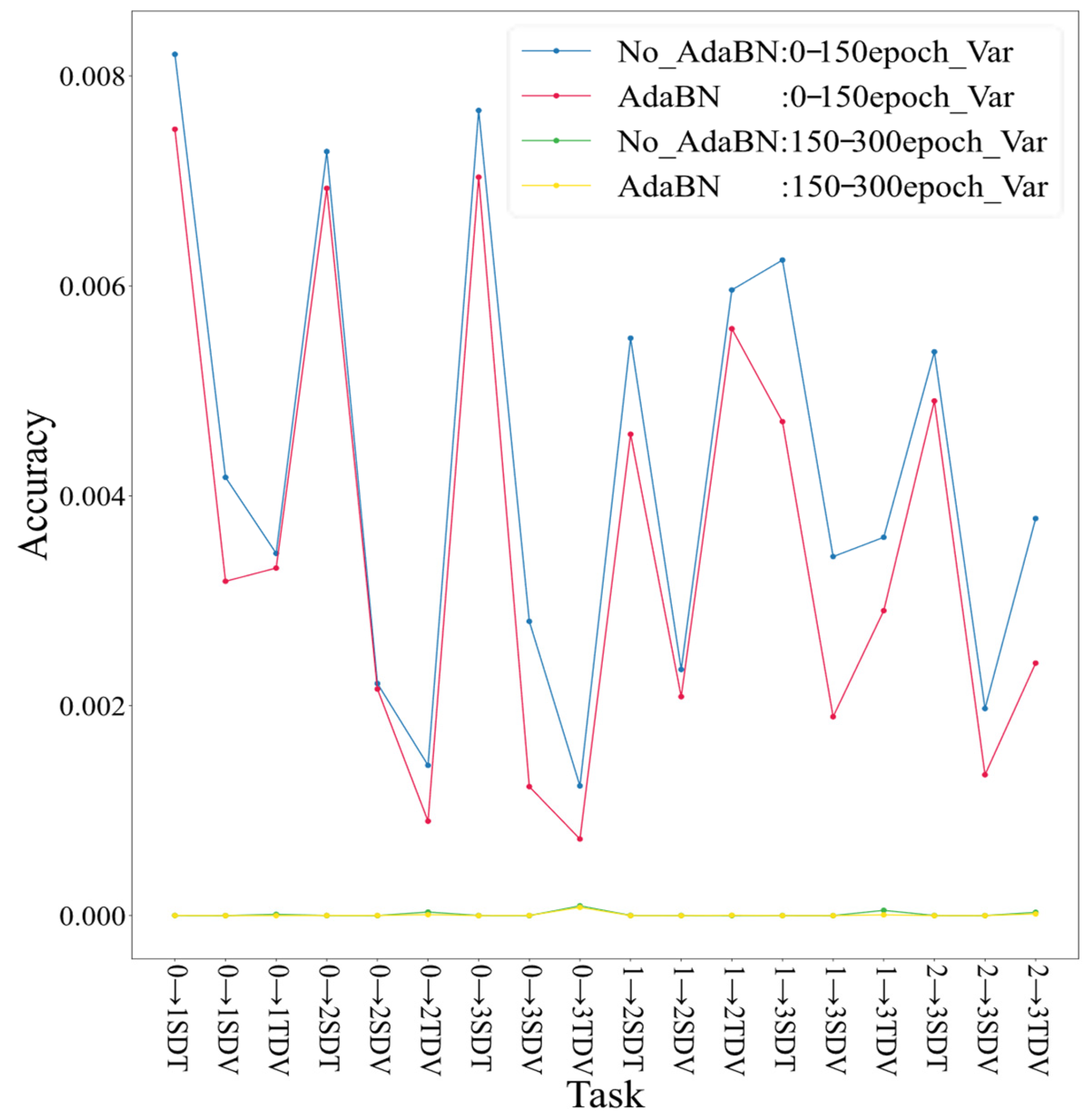
The improved BN algorithm proposed in this paper is experimentally verified using the CWRU dataset. Dividing the data into four groups, the rotation speed corresponds to 1797 rpm, 1772 rpm, 1750 rpm, and 1730 rpm, and the corresponding labels are 0, 1, 2, and 3, respectively. Each group contains 10 pieces of data, and these 10 pieces of data all include the original vibration signal of a normal bearing, the original vibration signal of an outer ring faulty bearing, the original vibration signal of an inner ring faulty bearing, and the original vibration signal of a rolling element faulty bearing. Figure 3 shows the accuracy rate of the model that migrated from the 0th group to the 1st group on the CWRU dataset; that is, the model migrated from the speed of 1797 rpm to 1772 rpm on the source domain training set and the source domain test set, respectively. Accuracy on the test set was found in the target domain. From Figure 3, we can see that the domain-adaptive diagnosis results based on AdaBN in the target domain are faster and more stable in the 0–150 epoch than the domain-adaptive diagnosis results without AdaBN, and the variance and mean are relatively larger. Domain-adaptive diagnosis results using AdaBN on epochs 150–300 have more stable convergence, relatively small variance, and higher accuracy. In order to verify the effectiveness and robustness of the method proposed in this paper, experiments were carried out for each transfer learning model under different rotational speeds, and a total of six groups of experiments were performed, namely: 0→1, 0→2, 0→3, 1→2, 1→3, and 2→3. Figure 4 is a line chart of six transition states, the abscissas correspond to six groups of experiments, and each experiment corresponds to the source training set (SDT) of the source domain, the source test set (SDV) of the source domain, and the target test set (TDV) of the target domain and target test set (TDV). The validation indicators include the mean and variance of the first 150 epochs and the mean and variance of the last 150 epochs. The model throughout the training process is trained on the training set of the source domain, the test set of the source domain, and the validation set of the target domain.
In this experiment, the authors computed the mean value of the first 150 epochs to evaluate whether using AdaBN could improve the initial accuracy of the model in the early stage of training. Additionally, authors measured the variance of the first 150 epochs and the last 150 epochs to investigate the stability of model at the beginning and end of training. The authors compared the variance of the two models when the average accuracy rate was similar to determine if the AdaBN model could provide better stability during the early stage of training. The results in Figure 4 demonstrate that using the AdaBN method generally resulted in higher accuracy than not using it in many training epochs.
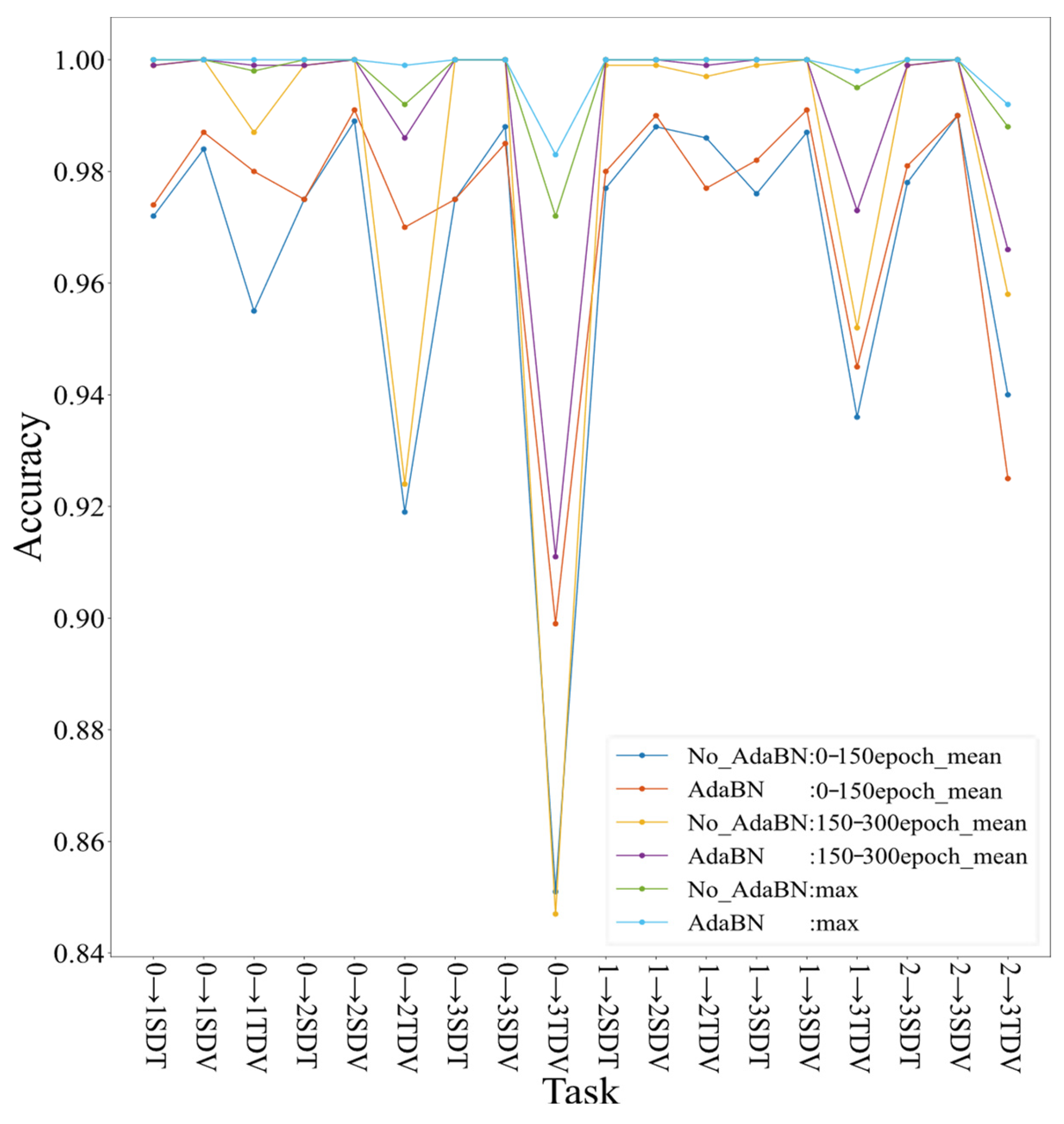
It can also be observed from Figure 5 that the variance with the AdaBN method is smaller than that without the AdaBN method. Variance is an important parameter that reflects the stability of the data, so, whether in the source domain or the target domain, the accuracy of transfer learning after using the AdaBN method is more stable. Figure 6 shows the mean and maximum values of the training set, the validation set of the source domain, and the validation set of the target domain under different transfer states on CWRU. Figure 7a shows the confusion matrix without AdaBN, and Figure 7b shows the confusion matrix with AdaBN. From the comparison of the two figures, it can be seen that the model without the AdaBN confusion matrix has a large number of misjudgments in Category 8. As shown in Table 3, our proposed method was first compared with traditional machine learning methods with six transfer conditions in detail. The results show that our proposed method outperforms the traditional SVM method by nearly 30%, the traditional MLP method by about 15%, and also has a stable improvement compared with our proposed method without AdaBN optimization. The AdaBN method proposed in this paper improves the accuracy of direct migration under different working conditions, which proves the effectiveness of the AdaBN method.
The main sources of error in this experiment are data collection, data preprocessing, model selection, and parameter tuning. In this experiment, parameter tuning is the main source of error, and different hyperparameters have a significant impact on the error of the model. Therefore, it is necessary to choose appropriate hyperparameters based on experience and actual conditions [38,39]. The key hyperparameters used in training the neural network in this paper are batch_size: 64, optim: Adam, learning_rate: 1 × 10⁻³, moment: 0.9, weight-decay: 1 × 10⁻⁵, lr_scheduler: Step, and epoch: 600.
2.
Validation on a laboratory testbed dataset
(1)
Introduction to the dataset
The tapered roller bearing used in this experiment was NUP205. The inner diameter was 25 mm, the outer diameter was 52 mm, and the width was 15 mm. The data were collected at seven different rotational speeds, and each rotational speed included normal bearing data, inner ring faulty bearing data, and outer ring faulty bearing data. Among them, 11 types of outer ring faults were designed, and 6 types of inner ring faults were designed. Two channels of data were collected in the horizontal and vertical directions for each specific type. In this paper, the vibration signal data in the horizontal direction at four different speeds of 900 rpm, 1200 rpm, 1500 rpm, and 1650 rpm were selected for the experiment. Figure 8 shows the experimental bench for simulating bearing data in the laboratory.
  • (2)
    Analysis of results
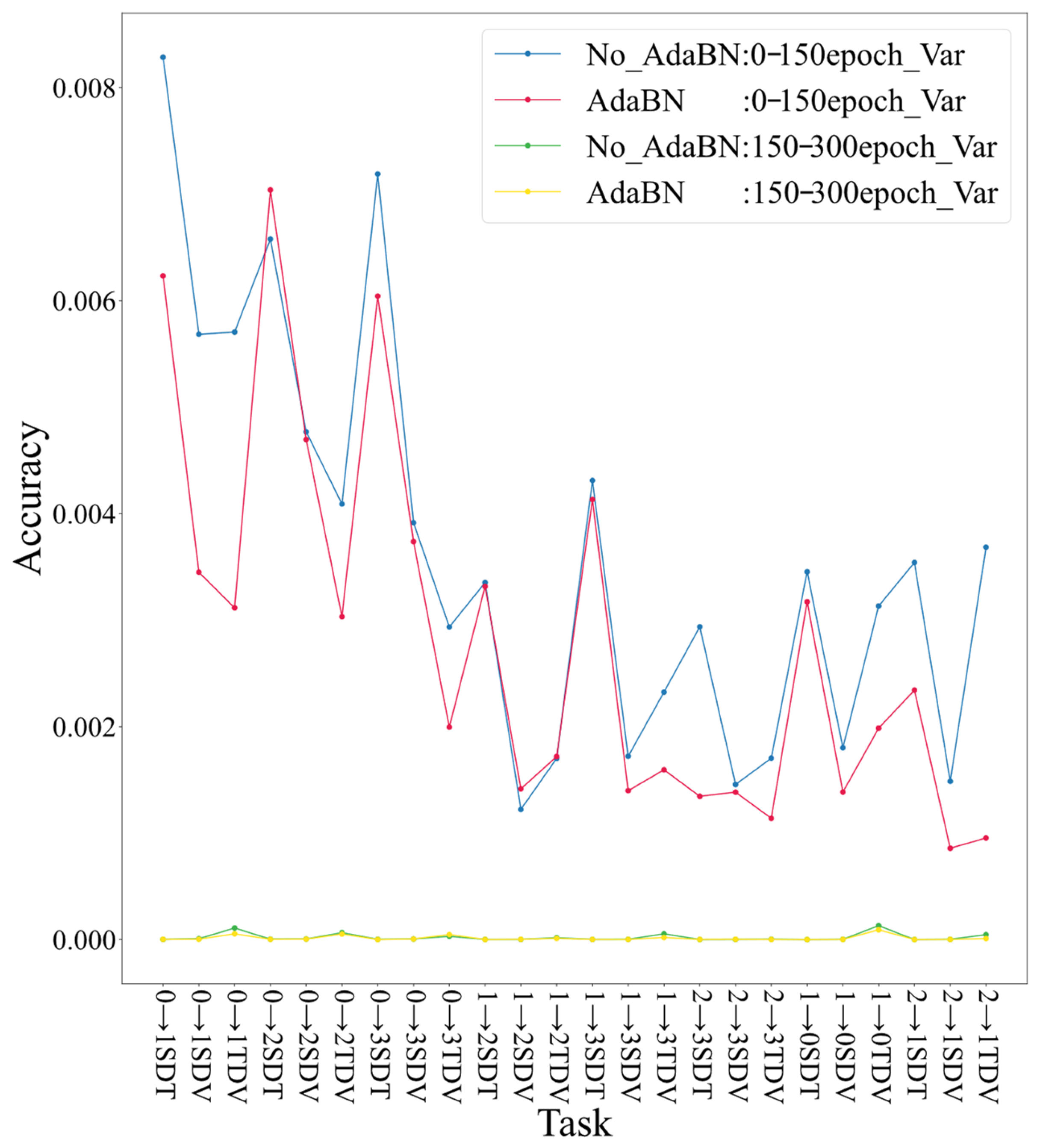
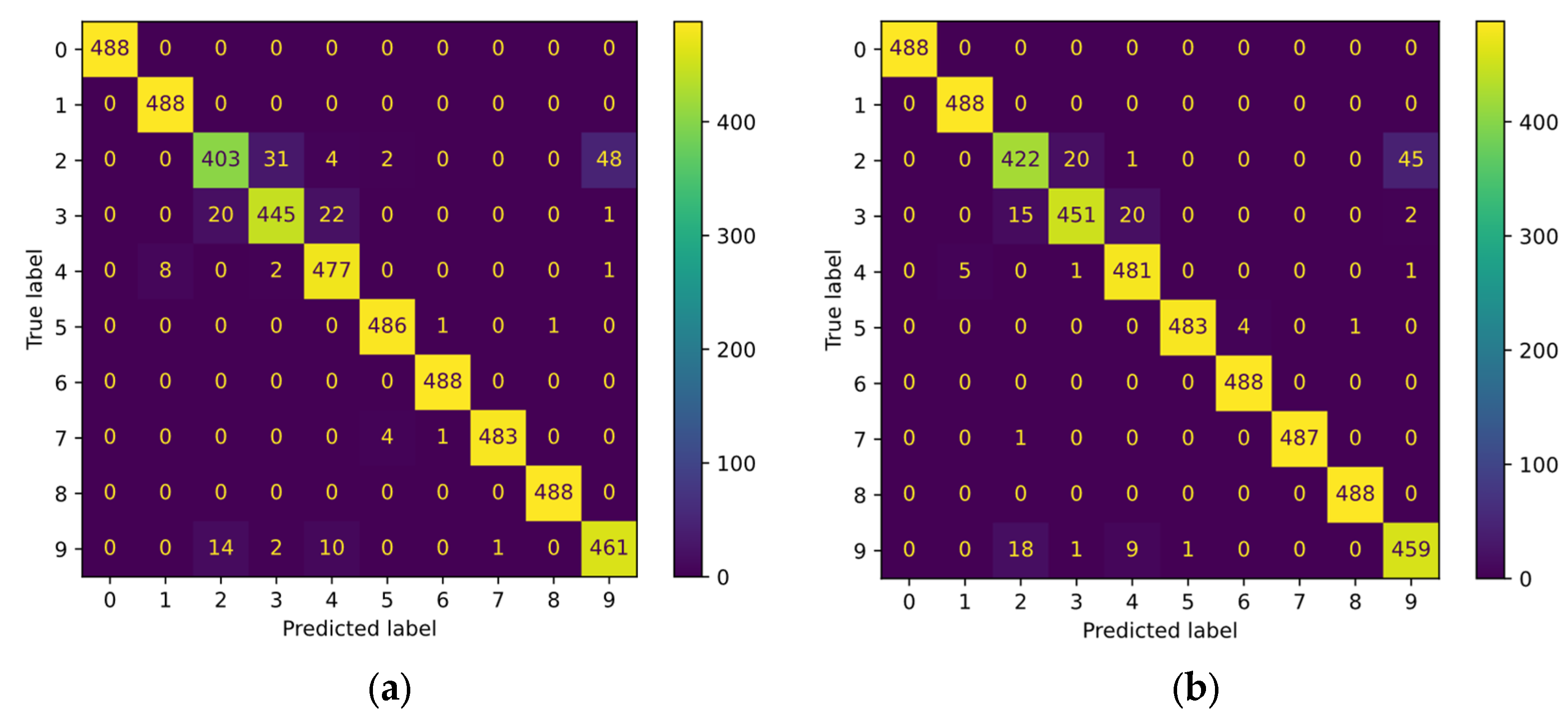
It can be seen from Table 4 that whether it is at a 0–150 epoch or 150–300 epoch, the accuracy of using the AdaBN method is obviously higher than that of using AdaBN on the laboratory test bench. It can be seen from Figure 9 that the variance of the AdaBN method is dominant in most transfer models, and it is better than the method without AdaBN in most cases. Therefore, using the AdaBN method in the bearing fault diagnosis migration model can improve the stability and accuracy of the model. The confusion matrix for never using AdaBN is shown in Figure 10a, and the confusion matrix for using AdaBN is shown in Figure 10b. Further, there are five more misclassifications other than those in Categories 5 and 9, namely, Categories 2, 3, 4, and 6. The exact number of use for the AdaBN method in Category 7 is much higher than that without using the AdaBN method. The effectiveness of the AdaBN method proposed in this paper is confirmed.

5. Conclusions

Sustainable energy is one of the most important research directions across various disciplines. In order to achieve timely detection of faults in rotary machinery during operation, this paper proposes a rotating machinery fault diagnosis method based on AdaBN adaptive domain generalization, which effectively improves the convergence speed and stability of the model. Compared with traditional machine learning methods, this method has higher accuracy and is beneficial for the timely diagnosis of faults in rotating machinery, thus promoting the sustainable development of energy. In the field of sustainability, adaptive batch normalization can also help detect faults in other mechanical equipment in the energy sector, thus promoting sustainable energy development. In addition to bearing fault diagnosis, adaptive batch normalization can also be used for tasks such as image classification, speech recognition, natural language processing, and sustainability. Adaptive batch normalization can enhance the generalization ability of different datasets, thus improving classification accuracy and enhancing the generalization ability of the model. In the future, the authors will continue to apply the AdaBN algorithm to the energy sector to promote sustainable energy development.

Author Contributions

Investigation, X.W.; resources, D.L.; writing—original draft, X.L. and T.Y.; visualization, C.S.; project administration, Z.X.; funding acquisition, X.K. All authors have read and agreed to the published version of the manuscript.

Funding

This work is supported in part by the Fundamental Research Funds for the Central Universities (No. 2572022BF07) and in part by the Key Laboratory of Vibration and Control of Aero-Propulsion System, Ministry of Education, Northeastern University (VCAME202209).

Institutional Review Board Statement

Not applicable.

Informed Consent Statement

Not applicable.

Data Availability Statement

Not applicable.

Conflicts of Interest

The authors declare no conflict of interest.

Abbreviation

Adaptive Batch NormalizationAdaBN
Wavelet TransformWT
Empirical Mode DecompositionEMD
Singular Value DecompositionSVD
Short-Time Fourier TransformSTFT
Support Vector MachinesSVM
Artificial Neural NetworkANN
Restricted Boltzmann MachinesRBM
Convolutional Neural NetworksCNN
Deep Belief NetworkDBN
Stacked AutoencodersSAE
Balanced Distribution AdaptationBDA
Kullback–LeiblerKL
Maximum Mean DiscrepancyMMD
Joint Distribution AdaptationJDA
Electric Discharge MachiningEDM
Batch NormalizationBN
Deep Convolutional Neural NetworksDCNN
Source training setSDT
Source test setSDV
Target test setTDV
Case Western Reserve UniversityCWRU

References

  1. Singh, N.; Hamid, Y.; Juneja, S.; Srivastava, G.; Dhiman, G.; Gadekallu, T.R.; Shah, M.A. Load balancing and service discovery using Docker Swarm for microservice based big data applications. J. Cloud Comput. 2023, 12, 1–9. [Google Scholar] [CrossRef]
  2. Slathia, S.; Kumar, R.; Lone, M.; Viriyasitavat, W.; Kaur, A.; Dhiman, G. A Performance Evaluation of Situational-Based Fuzzy Linear Programming Problem for Job Assessment. In Proceedings of Third International Conference on Advances in Computer Engineering and Communication Systems; ICACECS 2022; Springer: Berlin/Heidelberg, Germany, 2023; pp. 655–667. [Google Scholar]
  3. Tan, D.; Meng, Y.; Tian, J.; Zhang, C.; Zhang, Z.; Yang, G.; Cui, S.; Hu, J.; Zhao, Z. Utilization of renewable and sustainable diesel/methanol/n-butanol (DMB) blends for reducing the engine emissions in a diesel engine with different pre-injection strategies. Energy 2023, 269, 126785. [Google Scholar] [CrossRef]
  4. Tan, D.; Wu, Y.; Lv, J.; Li, J.; Ou, X.; Meng, Y.; Lan, G.; Chen, Y.; Zhang, Z. Performance optimization of a diesel engine fueled with hydrogen/biodiesel with water addition based on the response surface methodology. Energy 2023, 263, 125869. [Google Scholar] [CrossRef]
  5. Hu, J.; Zhang, L. Risk based opportunistic maintenance model for complex mechanical systems. Expert Syst. Appl. 2014, 41, 3105–3115. [Google Scholar] [CrossRef]
  6. Bao, J.; Qu, P.; Wang, H.; Zhou, C.; Zhang, L.; Shi, C. Implementation of various bowl designs in an HPDI natural gas engine focused on performance and pollutant emissions. Chemosphere 2022, 303, 135275. [Google Scholar] [CrossRef]
  7. Shi, C.; Chai, S.; Di, L.; Ji, C.; Ge, Y.; Wang, H. Combined experimental-numerical analysis of hydrogen as a combustion enhancer applied to Wankel engine. Energy 2023, 263, 125896. [Google Scholar] [CrossRef]
  8. Lei, Y.; Yang, B.; Jiang, X.; Jia, F.; Li, N.; Nandi, A.K. Applications of machine learning to machine fault diagnosis: A review and roadmap. Mech. Syst. Signal Process. 2020, 138, 106587. [Google Scholar] [CrossRef]
  9. Peng, T.; Gui, W.; Wu, M.; Xie, Y. A fusion diagnosis approach to bearing faults. In Proceedings of the International Conference on Modeling and Simulation in Distributed Applications, Changsha, China, 25–27 September 2001; pp. 759–766. [Google Scholar]
  10. Lei, Y.; Zuo, M.J.; He, Z.; Zi, Y. A multidimensional hybrid intelligent method for gear fault diagnosis. Expert Syst. Appl. 2010, 37, 1419–1430. [Google Scholar] [CrossRef]
  11. Stewart, G.W. On the early history of the singular value decomposition. SIAM Rev. 1993, 35, 551–566. [Google Scholar] [CrossRef]
  12. Griffin, D.; Lim, J. Signal estimation from modified short-time Fourier transform. IEEE Trans. Acoust. Speech Signal Process. 1984, 32, 236–243. [Google Scholar] [CrossRef]
  13. Cortes, C.; Vapnik, V. Support-vector networks. Mach. Learn. 1995, 20, 273–297. [Google Scholar] [CrossRef]
  14. Schmidhuber, J. Deep learning in neural networks: An overview. Neural Netw. 2015, 61, 85–117. [Google Scholar] [CrossRef] [PubMed]
  15. Cover, T.; Hart, P. Nearest neighbor pattern classification. IEEE Trans. Inf. Theory 1967, 13, 21–27. [Google Scholar] [CrossRef]
  16. Song, Y.-Y.; Ying, L. Decision tree methods: Applications for classification and prediction. Shanghai Arch. Psychiatry 2015, 27, 130. [Google Scholar]
  17. Glorot, X.; Bengio, Y. Understanding the difficulty of training deep feedforward neural networks. In Proceedings of the Thirteenth International Conference on Artificial Intelligence and Statistics, Sardinia, Italy, 13–15 May 2010; JMLR Workshop and Conference Proceedings. pp. 249–256. [Google Scholar]
  18. Rumelhart, D.E.; Hinton, G.E.; Williams, R.J. Learning representations by back-propagating errors. Nature 1986, 323, 533–536. [Google Scholar] [CrossRef]
  19. Albawi, S.; Mohammed, T.A.; Al-Zawi, S. Understanding of a convolutional neural network. In Proceedings of the 2017 International Conference on Engineering and Technology (ICET), Antalya, Turkey, 21–23 August 2017; IEEE: Piscataway, NJ, USA, 2017; pp. 1–6. [Google Scholar]
  20. Hua, Y.; Guo, J.; Zhao, H. Deep belief networks and deep learning. In Proceedings of the 2015 International Conference on Intelligent Computing and Internet of Things, Harbin, China, 17–18 January 2015; IEEE: Piscataway, NJ, USA, 2015; pp. 1–4. [Google Scholar]
  21. Wu, Z.; Shen, C.; Van Den Hengel, A. Wider or deeper: Revisiting the resnet model for visual recognition. Pattern Recognit. 2019, 90, 119–133. [Google Scholar] [CrossRef]
  22. Zhong, S.; Fu, S.; Lin, L. A novel gas turbine fault diagnosis method based on transfer learning with CNN. Measurement 2019, 137, 435–453. [Google Scholar] [CrossRef]
  23. Zhao, B.; Zhang, X.; Zhan, Z.; Pang, S. Deep multi-scale convolutional transfer learning network: A novel method for intelligent fault diagnosis of rolling bearings under variable working conditions and domains. Neurocomputing 2020, 407, 24–38. [Google Scholar] [CrossRef]
  24. Wang, K.; Wu, B. Power equipment fault diagnosis model based on deep transfer learning with balanced distribution adaptation. In Proceedings of the International Conference on Advanced Data Mining and Applications, Nanjing, China, 16–18 November 2018; Springer: Berlin/Heidelberg, Germany, 2018; pp. 178–188. [Google Scholar]
  25. Wang, Y.; Wang, C.; Kang, S.; Xie, J.; Wang, Q.; Mikulovich, V. Network-combined broad learning and transfer learning: A new intelligent fault diagnosis method for rolling bearings. Meas. Sci. Technol. 2020, 31, 115013. [Google Scholar] [CrossRef]
  26. Yang, B.; Lei, Y.; Jia, F.; Li, N.; Du, Z. A polynomial kernel induced distance metric to improve deep transfer learning for fault diagnosis of machines. IEEE Trans. Ind. Electron. 2019, 67, 9747–9757. [Google Scholar] [CrossRef]
  27. Han, T.; Liu, C.; Yang, W.; Jiang, D. Deep transfer network with joint distribution adaptation: A new intelligent fault diagnosis framework for industry application. ISA Trans. 2020, 97, 269–281. [Google Scholar] [CrossRef] [PubMed]
  28. Qian, W.; Li, S.; Yi, P.; Zhang, K. A novel transfer learning method for robust fault diagnosis of rotating machines under variable working conditions. Measurement 2019, 138, 514–525. [Google Scholar] [CrossRef]
  29. Li, Y.; Song, Y.; Jia, L.; Gao, S.; Li, Q.; Qiu, M. Intelligent fault diagnosis by fusing domain adversarial training and maximum mean discrepancy via ensemble learning. IEEE Trans. Ind. Inform. 2020, 17, 2833–2841. [Google Scholar] [CrossRef]
  30. Zhang, Y.; Ren, Z.; Zhou, S. A new deep convolutional domain adaptation network for bearing fault diagnosis under different working conditions. Shock. Vib. 2020, 2020, 8850976. [Google Scholar] [CrossRef]
  31. Shao, H.; Zhang, X.; Cheng, J.; Yang, Y. Intelligent fault diagnosis of bearing using enhanced deep transfer auto-encoder. J. Mech. Eng. 2020, 56, 84–91. [Google Scholar]
  32. Li, C.-L.; Chang, W.-C.; Cheng, Y.; Yang, Y.; Póczos, B. Mmd gan: Towards deeper understanding of moment matching network. Adv. Neural Inf. Process. Syst. 2017, 30. [Google Scholar] [CrossRef]
  33. Ioffe, S.; Szegedy, C. Batch normalization: Accelerating deep network training by reducing internal covariate shift. In Proceedings of the International Conference on Machine Learning, Lille, France, 6–11 July 2015; PMLR: New York, NY, USA, 2015; pp. 448–456. [Google Scholar]
  34. He, K.; Zhang, X.; Ren, S.; Sun, J. Deep residual learning for image recognition. In Proceedings of the IEEE Conference on Computer Vision and Pattern Recognition, Las Vegas, NV, USA, 27–30 June 2016; pp. 770–778. [Google Scholar]
  35. Li, X.; Su, K.; He, Q.; Wang, X. Research on fault diagnosis of highway bi-lstm based on attention mechanism. Eksploat. I Niezawodn.-Maint. Reliab. 2023, 25. [Google Scholar] [CrossRef]
  36. Li, J.; He, D. A Bayesian optimization AdaBN-DCNN method with self-optimized structure and hyperparameters for domain adaptation remaining useful life prediction. IEEE Access 2020, 8, 41482–41501. [Google Scholar] [CrossRef]
  37. Li, Y.; Wang, N.; Shi, J.; Liu, J.; Hou, X. Revisiting batch normalization for practical domain adaptation. arXiv 2016, arXiv:1603.04779. [Google Scholar]
  38. Huang, L. Normalization ináTask-Specific Applications. In Normalization Techniques in Deep Learning; Springer: Berlin/Heidelberg, Germany, 2022; pp. 87–100. [Google Scholar]
  39. Jin, T.; Yan, C.; Chen, C.; Yang, Z.; Tian, H.; Guo, J. New domain adaptation method in shallow and deep layers of the CNN for bearing fault diagnosis under different working conditions. Int. J. Adv. Manuf. Technol. 2023, 124, 3701–3712. [Google Scholar] [CrossRef]
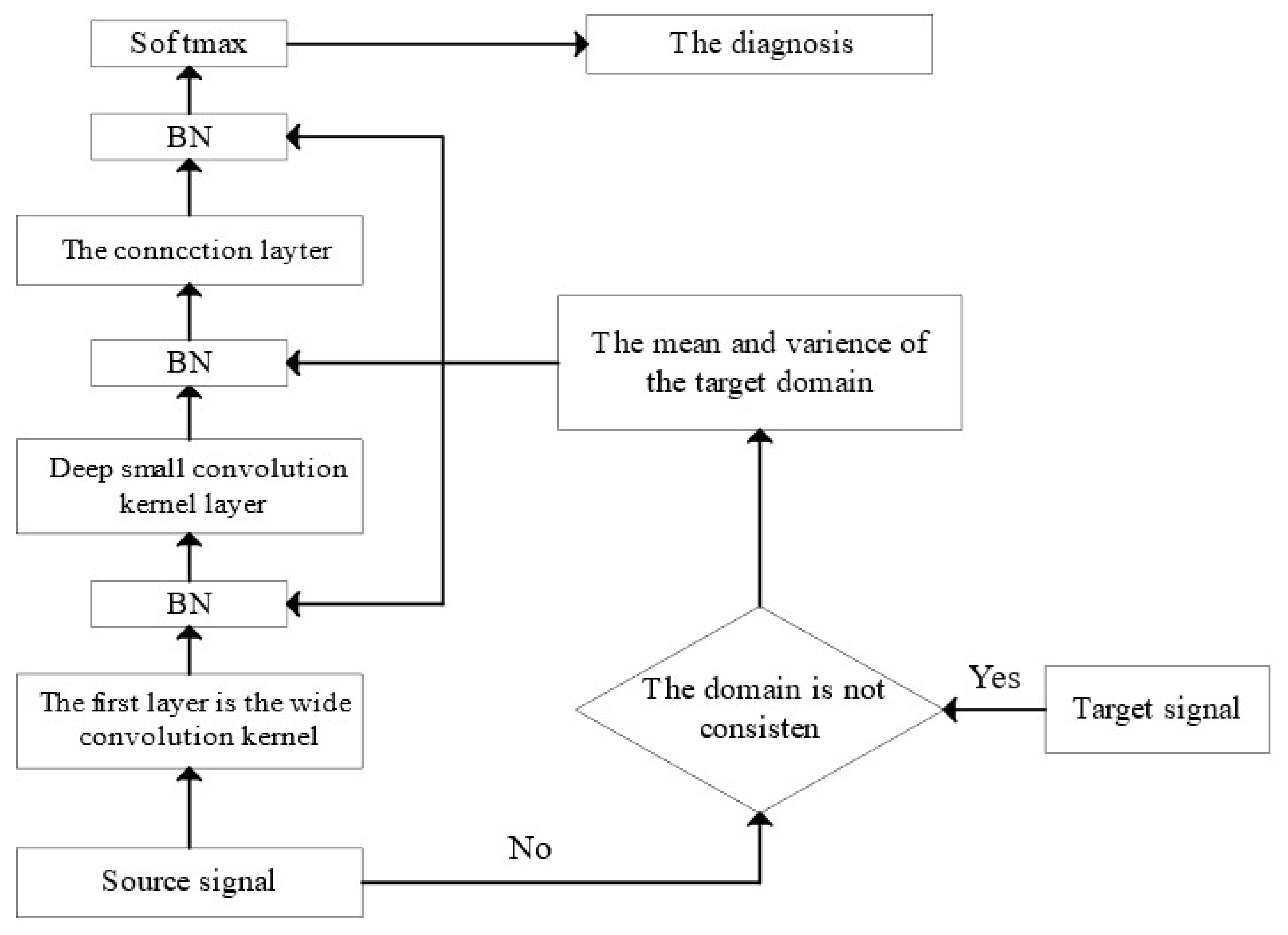
Figure 1. The flowchart of the AdaBN algorithm proposed for fault diagnosis.
Sustainability 15 08034 g001
Figure 2. DCNN network architecture diagram.
Sustainability 15 08034 g002
Figure 3. CWRU rolling bearing data acquisition system.
Sustainability 15 08034 g003
Figure 4. (a) Accuracy rate in each domain using the AdaBN method. (b) Accuracy rate in each domain without using the AdaBN method.
Sustainability 15 08034 g004
Figure 5. The variance on the CWRU dataset.
Sustainability 15 08034 g005
Figure 6. The accuracy of the mean and maximum value in different domains on the CWRU dataset.
Sustainability 15 08034 g006
Figure 7. (a) Confusion matrix without AdaBN on CWRU dataset. (b) Confusion matrix with AdaBN on CWRU dataset.
Sustainability 15 08034 g007
Figure 8. The data acquisition test bench for the laboratory dataset.
Sustainability 15 08034 g008
Figure 9. The variance on the laboratory dataset.
Sustainability 15 08034 g009
Figure 10. (a) Confusion matrix without AdaBN on laboratory dataset. (b) Confusion matrix with AdaBN on laboratory dataset.
Sustainability 15 08034 g010
Table 1. DCNN algorithm based on AdaBN domain adaptation.
AlgorithmDCNN Algorithm Based on AdaBN Domain Adaptive
EnterSignal p of the target domain, expressed in the i neuron of the BN layer of the DCNN x t ( i ) ( p ) x t ( i ) of which x t ( i ) = x t ( i ) ( 1 ) , , x t ( i ) ( n ) , for the i neuron, has been trained to scale with parallel parameters γ s ( i ) and β s ( i ) .
OutputThe adjusted DCNN network
ForFor each neuron i and each signal p in the target domain, compute the mean and variance of all samples in the target domain:
μ t ( i ) E x t ( i )
σ t ( i ) V a r x t ( i )
Calculate the output of the BN layer:
x ^ t ( i ) ( p ) = x t ( i ) ( p ) μ t ( i ) σ t ( i )
y t ( i ) ( p ) = γ s ( i ) x ^ t ( i ) ( p ) + β s ( i )
End for
Table 2. One-dimensional neural network structure parameters.
NumberNetwork
Layer
Kernel Size/StepNumber of KernelOutput Size (Width × Depth)
1Conv11 × 15/1161 × 1010
2Conv21 × 3/1321 × 1008
3Pool11 × 2/2321 × 504
4Conv31 × 3/1641 × 504
5Conv41 × 3/11281 × 502
6AdaptiveMaxpool41281 × 4
7Fc 1————512
8Fc 2————256
9Fc 3————256
10Fc 4————10
Table 3. Comparison of accuracy of each algorithm in six migration states.
Task0→10→20→31→21→32→3
SVM70.34%74.23%71.23%68.45%73.12%68.49%
MLP85.24%82.93%80.98%78.21%84.82%88.49%
DCNN99.12%98.89%97.53%99.59%99.53%98.53%
DCNN (AdaBN)99.89%99.85%98.83%99.59%99.82%99.12%
Table 4. The mean and maximum values under different migration states.
TaskNo_AdaBNAdaBNNo_AdaBNAdaBNNo_AdaBNAdaBN
0–150
Epoch
Mean
0–150
Epoch
Mean
150–300
Epoch
Mean
150–300
Epoch
Mean
0–300
Epoch
Max
0–300
Epoch Max
0→10.8330.8690.8620.8830.9510.952
0→20.9420.9480.9960.9980.9990.999
0→30.9040.9050.9420.9480.9460.956
1→20.7440.8110.7650.8240.8530.900
1→30.9360.9440.9970.9990.9991.000
2→30.9020.9040.9510.9500.9560.955
1→00.7230.7810.7300.7800.8380.890
2→10.9660.9600.9990.9991.0001.000
Disclaimer/Publisher’s Note: The statements, opinions and data contained in all publications are solely those of the individual author(s) and contributor(s) and not of MDPI and/or the editor(s). MDPI and/or the editor(s) disclaim responsibility for any injury to people or property resulting from any ideas, methods, instructions or products referred to in the content.